Rapid computations of spectrotemporal prediction error support perception of degraded speech
- School of Psychology, University of Sussex, United Kingdom
- MRC Cognition and Brain Sciences Unit, United Kingdom
Figures
Figure 1 with 1 supplement

Overview of experimental design and hypotheses.
(A) On each trial, listeners heard and judged the clarity of a degraded spoken word. Listeners’ prior knowledge of speech content was manipulated by presenting matching (‘clay’) or mismatching (‘fast’) text before spoken words presented with varying levels of sensory detail (3/6/12-channel vocoded), panel reproduced from B, Sohoglu and Davis, 2016. (B) Ratings of speech clarity were enhanced not only by increasing sensory detail but also by prior knowledge from matching text (graph reproduced from Figure 2A, Sohoglu and Davis, 2016). Error bars represent the standard error of the mean after removing between-subject variance, suitable for repeated-measures comparisons (Loftus and Masson, 1994). (C) Schematic illustrations of two representational schemes by which prior knowledge and speech input are combined (for details, see Materials and methods section). For illustrative purposes, we depict degraded speech as visually degraded text. Under a sharpening scheme (left panels), neural representations of degraded sensory signals (bottom) are enhanced by matching prior knowledge (top) in the same way as perceptual outcomes are enhanced by prior knowledge. Under a prediction error scheme (right panels), neural representations of expected speech sounds are subtracted from sensory signals. These two schemes make different predictions for experiments that assess the content of neural representations when sensory detail and prior knowledge of speech are manipulated. (D) Theoretical predictions for sharpened signal (left) and prediction error (right) models. In a sharpened signal model, representations of the heard spoken word (e.g. ‘clay’; expressed as the squared correlation with a clear [noise-free] ‘clay’) are most accurately encoded in neural responses when increasing speech sensory detail and matching prior knowledge combine to enhance perception. Conversely, for models that represent prediction error, an interaction between sensory detail and prior knowledge is observed. For speech that mismatches with prior knowledge, increasing sensory detail results in better representation of the heard word ‘clay’ because bottom-up input remains unexplained. Conversely, for speech that matches prior knowledge, increased sensory detail results in worse encoding of ‘clay’ because bottom-up input is explained away. Note that while the overall magnitude of prediction error is always the smallest when expectations match with speech input (see Figure 1—figure supplement 1), the prediction error representation of matching ‘clay’ is enhanced for low-clarity speech and diminished for high-clarity speech. For explanation, see the Discussion section.
© 2016, PNAS. Figure 1A reproduced from Figure 1B, Sohoglu and Davis, 2016. The author(s) reserves the right after publication of the WORK by PNAS, to use all or part of the WORK in compilations or other publications of the author's own works, to use figures and tables created by them and contained in the WORK.
© 2016, PNAS. Figure 1B reproduced from Figure 2A, Sohoglu and Davis, 2016. The author(s) reserves the right after publication of the WORK by PNAS, to use all or part of the WORK in compilations or other publications of the author's own works, to use figures and tables created by them and contained in the WORK.
Figure 1—figure supplement 1

Summed absolute prediction error for representations illustrated in Figure 1C.
Figure 2
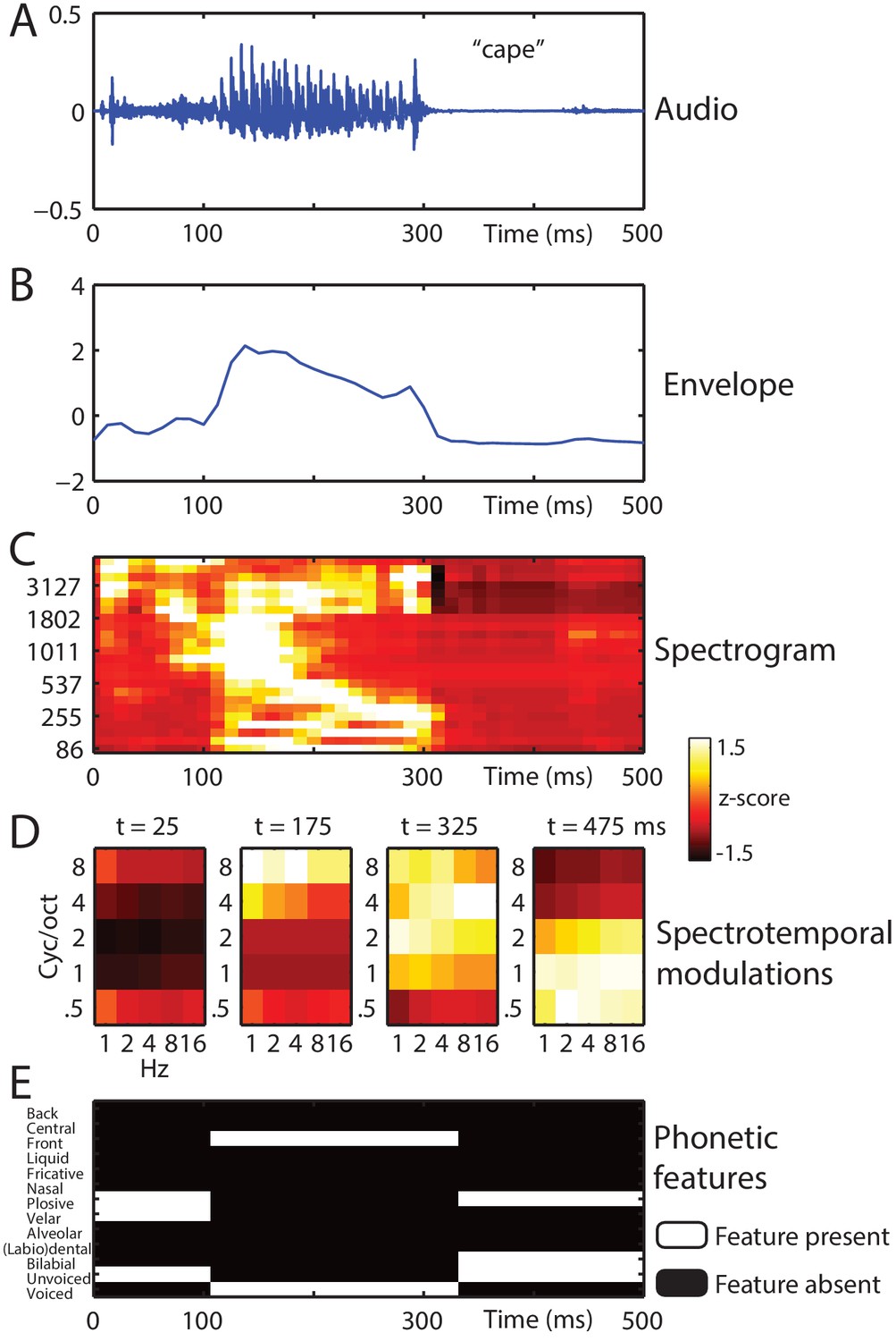
Stimulus feature spaces used to model MEG responses, for the example word ‘cape’.
(A) shown as an audio waveform for the original clear recording (i.e. before vocoding). (B) Envelope: broadband envelope derived from summing the envelopes across all spectral channels of a 24-channel noise-vocoder. (C) Spectrogram: derived from the envelope in each spectral channel of a 24-channel noise-vocoder. (D) Spectrotemporal modulations: derived from the spectral and temporal decomposition of a spectrogram into 25 spectrotemporal modulation channels, illustrated at regular temporal intervals through the spoken word. (E) Phonetic features: derived from segment-based representations of spoken words.
Figure 3 with 1 supplement

Encoding model comparison.
(A) Mean model accuracies for the four feature spaces (black bars) and the two feature space combinations (white bars). Error bars represent the standard error of the mean after removing between-subject variance, suitable for repeated-measures comparisons (Loftus and Masson, 1994). Braces indicate the significance of paired t-tests ***p<0.001 (B) Topographic distribution of MEG gradiometer sensors over which model accuracies were averaged. In each hemisphere of each participant, we selected 20 sensors with the highest model accuracies. The topographies show the percentage of participants for which each sensor was selected, consistent with neural sources in the superior temporal cortex.
Figure 3—figure supplement 1

Increases in model accuracy when combining feature spaces.
(A) Performance gain when adding feature spaces to the spectrogram. Green asterisks indicate p-values from one-sample t-tests comparing each feature space combination against the spectrogram alone. Black asterisks and braces indicate p-values from paired t-tests. Error bars represent the standard error of the mean. (B) Same as panel A but when adding feature spaces to spectrotemporal modulations.
Figure 4

Acoustic comparison of vocoded speech stimuli at varying levels of sensory detail.
(A) The magnitude of different spectrotemporal modulations for speech vocoded with different numbers of channels and clear speech (for comparison only; clear speech was not presented to listeners in the experiment). (B) Mean between-word Euclidean distance for different spectrotemporal modulations in speech vocoded with different numbers of channels. (C) Paired t-test showing significant differences in spectrotemporal modulation magnitude for comparison of 958 spoken words vocoded with 24 channels versus one channel (p<0.05 FDR corrected for multiple comparisons across spectrotemporal modulations). (D) Mean difference of between-word Euclidean distances for different spectrotemporal modulations for 24 versus 1 channel vocoded speech.
Figure 5 with 1 supplement
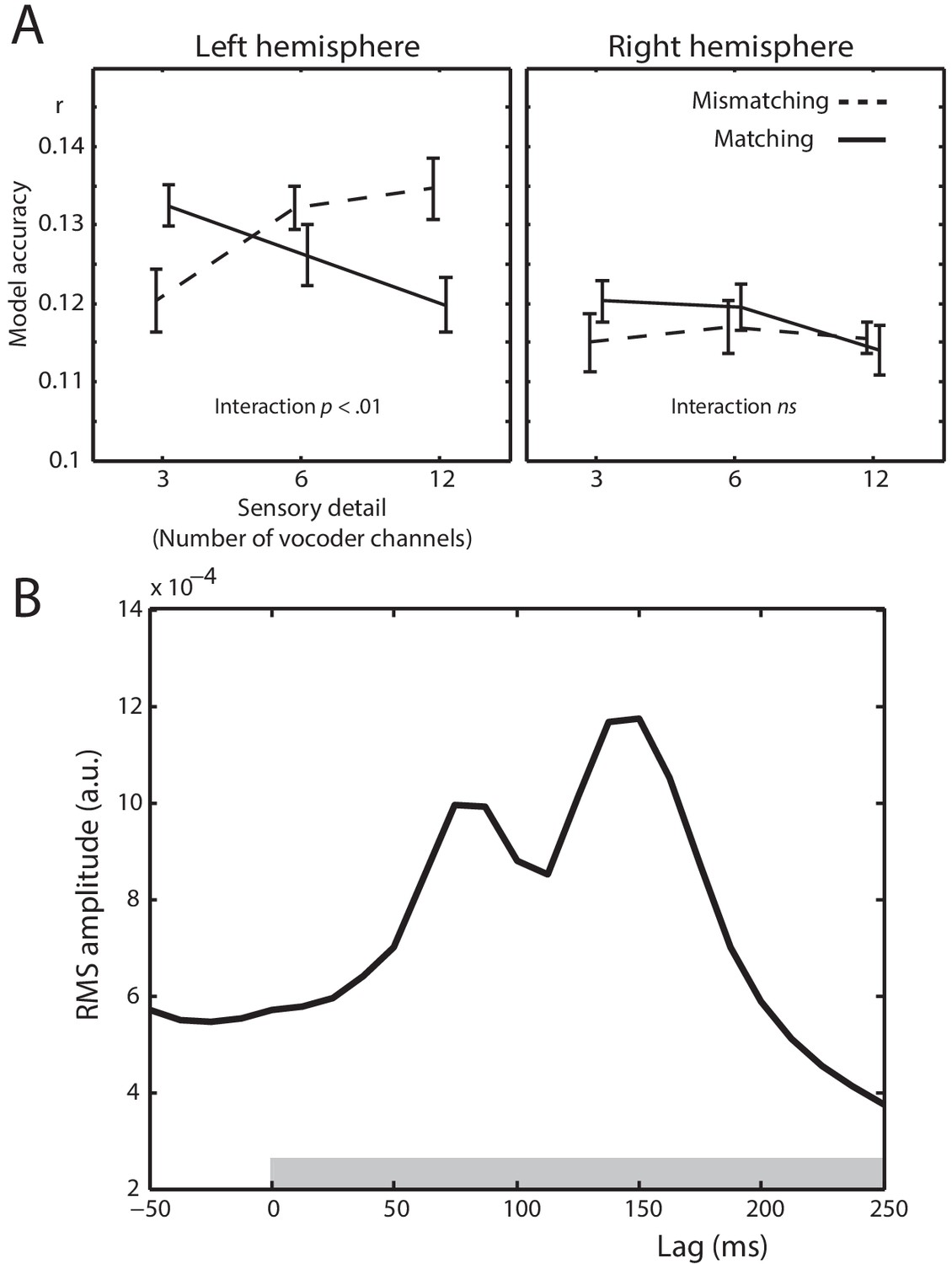
Spectrotemporal modulation encoding model results.
(A) Mean model accuracies for lags between 0 and 250 ms as a function of sensory detail (3/6/12 channel vocoded words), and prior knowledge (speech after mismatching/matching text) in the left and right hemisphere sensors. Error bars represent the standard error of the mean after removing between-subject variance, suitable for repeated-measures comparisons (Loftus and Masson, 1994). (B) Root Mean Square (RMS) amplitude across all left hemisphere sensors for the Temporal Response Functions (TRFs) averaged over spectrotemporal modulations, conditions, and participants. The gray box at the bottom of the graph indicates the lags used in computing the model accuracy data in panel A.
Figure 5—figure supplement 1
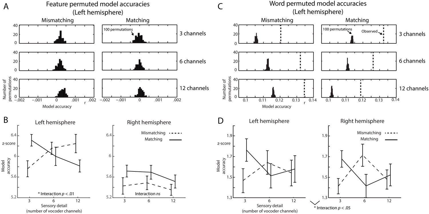
Control analysis of encoding model accuracies.
(A) Histograms of model accuracies in the left hemisphere sensors when fully permuting the feature representation of each spoken word. Histograms show the number of permutations a model accuracy was observed. (B) Model accuracies when z-scoring the observed model accuracies in Figure 5A with respect to the f-shuffled distributions in A. (C) Same as panel A but when permuting the feature representations across trials (i.e. shuffling the words in our stimulus set). Broken vertical lines show the mean observed model accuracies (in the left hemisphere sensors) from Figure 5A. (D) Model accuracies when z-scoring with respect to the word-shuffled distributions in C.
Figure 6 with 1 supplement
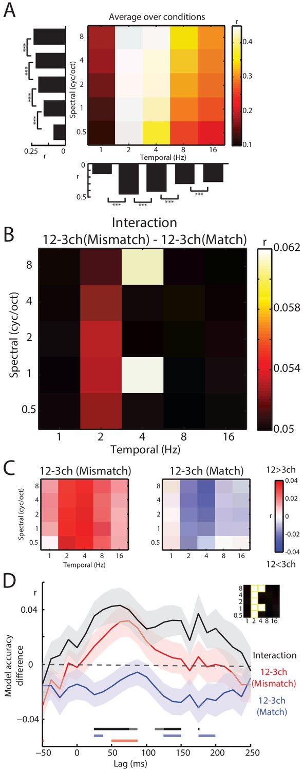
Decoding of spectrotemporal modulations from MEG responses to speech.
(A) The grid shows model accuracies for specific spectrotemporal modulations averaged over conditions. The left bar graph depicts model accuracy for each spectral modulation frequency, averaged over temporal modulations. Bottom bar graph depicts model accuracy for each temporal modulation frequency, averaged over spectral modulations. Braces indicate the significance of paired t-tests ***p<0.001 (B) Effect size (model accuracy differences, r) for the interaction contrast: 12–3 channels (Mismatch) – 12–3 channels (Match). The effect size display has been thresholded so as to only show cells in which the sensory detail by prior knowledge interaction is statistically significant at p<0.05 FDR corrected for multiple comparisons across spectrotemporal modulations. (C) Effect size (model accuracy differences, r) for comparisons between 12 and 3 channels, computed separately for Mismatch and Match conditions. Red shows greater model accuracy for 12 channel than for three channel speech (observed for speech that Mismatches with written text). Blue shows lower model accuracy for 12 channel than for three channel speech (observed for speech that matches written text). ch = channels. (D) Timecourse of decoding accuracy (single-lag analysis). Black trace shows model accuracy differences (r) attributable to the interaction contrast 12–3 channels (Mismatch) – 12–3 channels (Match). Red and blue traces show the contrast 12–3 channels separately for Mismatch and Match conditions, respectively. Shading around each trace represents the standard error of the mean. Horizontal bars at the bottom indicate significant lags for each contrast using the same color scheme as the traces (dark sections indicate p<0.05 FDR corrected across lags and light sections indicate p<0.05 uncorrected). Data have been averaged over the spectrotemporal modulations showing a significant interaction in panel B, indicated also as an inset (top-right).
Figure 6—figure supplement 1

Timecourse of decoding accuracy (single-lag analysis).
Magenta and green traces show model accuracy differences (r) attributable to the contrast Match-Mismatch separately for 3 and 12 channel conditions, respectively. For comparison, we also display (as the black trace) the interaction contrast 12–3 channels (Mismatch) – 12–3 channels (Match), same as shown in Figure 6. Shading around each trace represents the standard error of the mean. Horizontal bars at the bottom indicate significant lags for each contrast using the same color scheme as the traces (dark sections indicate p<0.05 FDR corrected across lags and light sections indicate p<0.05 uncorrected). Data have been averaged over the spectrotemporal modulations showing a significant interaction in Figure 6B, indicated also as an inset (top-right).
Author response image 1
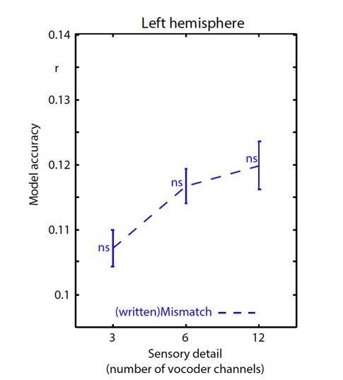
Encoding accuracy in left hemisphere sensors.
Data have been analyzed in an identical fashion to Figure 5A except that we show a new (written)Mismatch condition in which the spectrotemporal modulation representation of the written word is used to predict neural responses. There was a significant main effect of sensory detail for this (written)Mismatch condition (F(2,40) = 4.466 p = .023). However, as explained below, permutation testing in which we shuffled the order of the stimuli (over 100 permutations) revealed that each (written)Mismatch datapoint did not significantly differ from the permutation null distribution. ns p >=.05. This is in contrast to the match/mismatch conditions reported in the manuscript which all showed above-chance encoding accuracy for the spoken word that was heard irrespective of sensory clarity.
Author response image 2
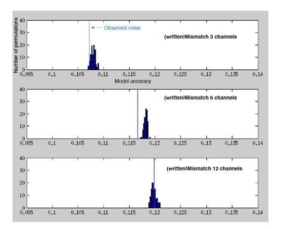
Histograms showing the number of permutations (random shuffles of feature space across trials) as a function of (binned) model accuracy when predicting the MEG response from the spectrotemporal modulation representation of mismatching text.
Vertical blue lines indicate the observed (non-permuted) model accuracies.
Author response image 3
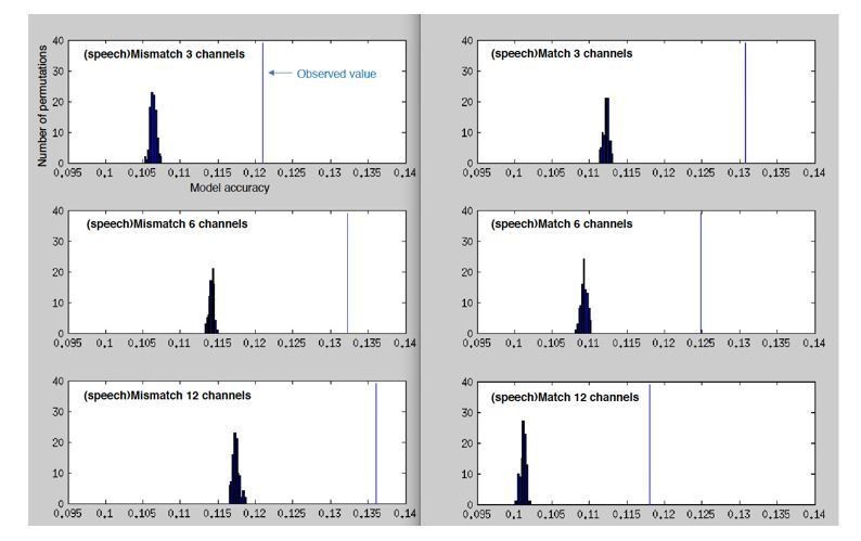
Histograms showing the number of permutations (random shuffles of feature space across trials) as a function of (binned) model accuracy when predicting the MEG response from the spectrotemporal modulation representation of mismatching/matching speech.
Vertical blue lines indicate the observed (non-permuted) model accuracies.
Author response image 4
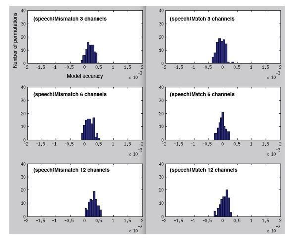
Histograms showing permutation null distributions when predicting the MEG response from the spectrotemporal modulation representation of mismatching/matching speech but now for a fully-permuted model (randomly permuting spectrotemporal modulation channels and time-bins).
Note the scale for these graphs is much smaller than the previous figures (-.002 to.002 versus.095 to.14), reflecting the substantial drop in model accuracy to near-zero for the fully permuted model.
Author response image 5
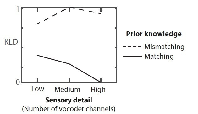
Kullback Liebler Divergence (KLD) between speech input and prediction patterns (shown in Figure 1C).
Additional files
Download links
A two-part list of links to download the article, or parts of the article, in various formats.
Downloads (link to download the article as PDF)
Open citations (links to open the citations from this article in various online reference manager services)
Cite this article (links to download the citations from this article in formats compatible with various reference manager tools)
Rapid computations of spectrotemporal prediction error support perception of degraded speech
eLife 9:e58077.
https://doi.org/10.7554/eLife.58077


