anTraX, a software package for high-throughput video tracking of color-tagged insects
- Laboratory of Social Evolution and Behavior, The Rockefeller University, United States
Figures
Figure 1
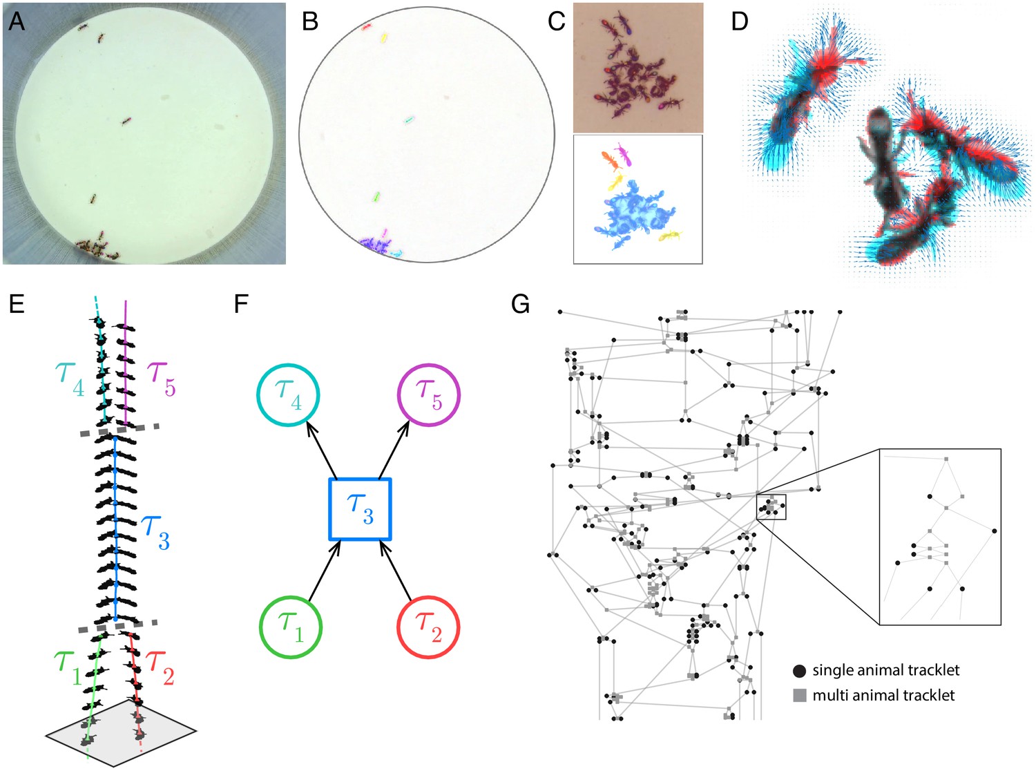
Blob tracking and construction of the tracklet graph.
(A) An example frame from an experiment with 16 ants marked with two color tags each. (B) The segmented frame after background subtraction. Each blob is marked with a unique color. Some blobs contain single ants, while others contain multiple ants. (C) A higher resolution segmentation example. While some ants are not distinguishable from their neighbors even for the human eye, others might be segmented by tuning the segmentation parameters, or by using other, more sophisticated segmentation algorithms. The anTraX algorithm takes a conservative approach and leaves those cases unsegmented to avoid segmentation errors. (D) Optical flow is used to estimate the ‘flow’ of pixels from one frame to the next, giving an approximation of the movements of the ants. The cyan silhouettes represent the location of an ant in the first frame, and the red silhouettes represent the location in the second frame. The results of the optical flow procedure are shown with blue arrows, depicting the displacement of pixels in the image. (E) An example of constructing and linking tracklets. Each layer represents a section of segmented frame. Two ants are approaching each other (tracklets marked τ1 and τ2), until they are segmented together. At that point, the two tracklets end, and a third multi-ant tracklet begins (τ3). Once the two ants are again segmented individually, the multi-ant tracklet ends, and two new single-ant tracklets begin (τ4 and τ5). (F) The graph representation of the tracklet example in E. (G) A tracklet graph from an experiment with 36 ants, representing 3 min of tracking data. The nodes are located according to the tracklet start time on the vertical axis, beginning at the bottom. The inset depicts a zoomed-in piece of the graph.
Figure 2 with 1 supplement
Tracklet classification and ID propagation on the tracklet graph.
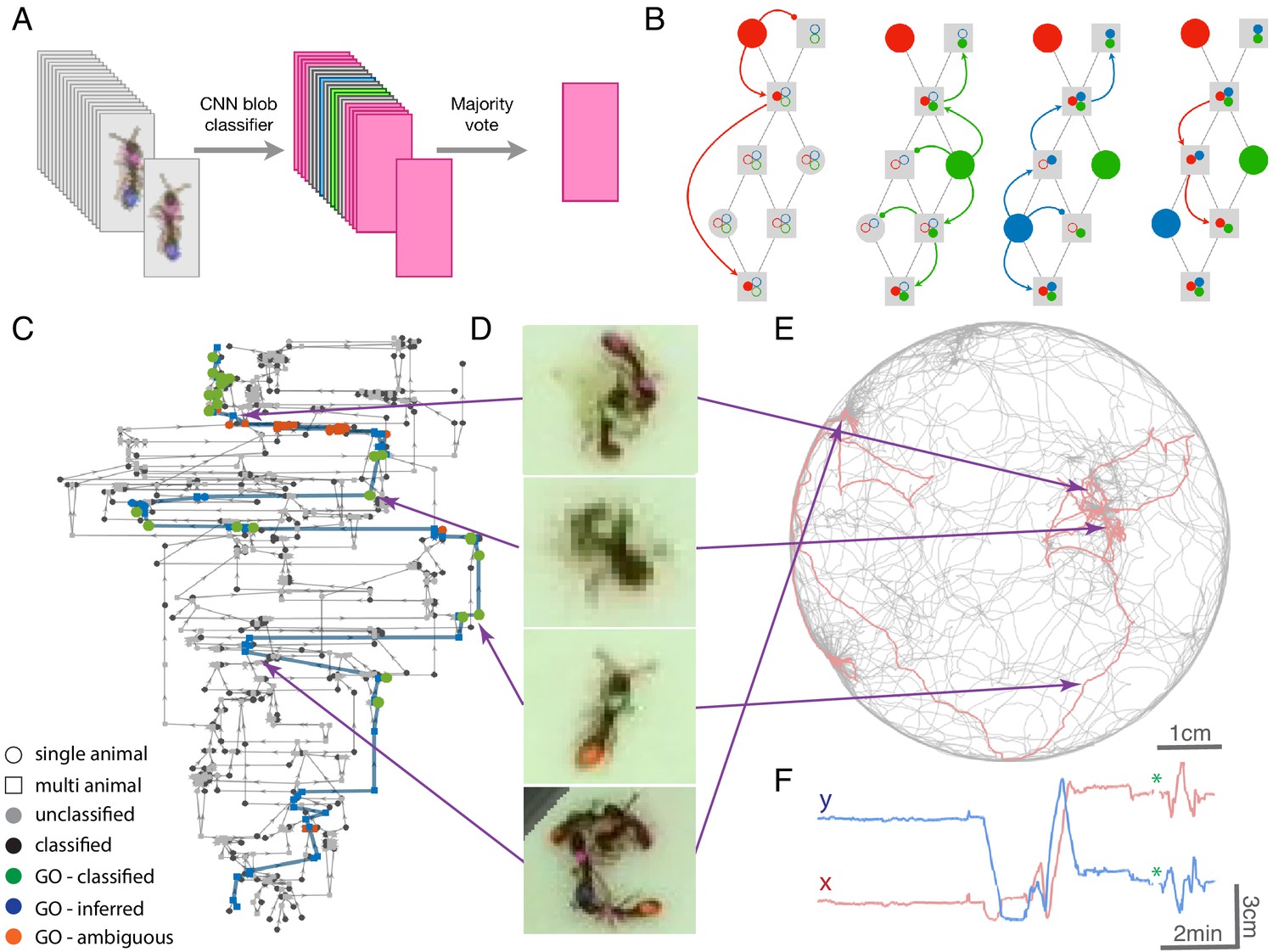
(A) Schematic of the tracklet classification procedure. All blobs belonging to the tracklet are classified by a pre-trained CNN classifier. The classifier assigns a label to each blob, which can be an individual ID (depicted as colored rectangles in the figure), or an ambiguous label (‘unknown’, depicted in gray). The tracklet is then classified as the most abundant ID in the label set, along with a confidence score that depends on the combination of blob classifications and their scores (see Supplementary Material for details). (B) A simple example of propagating IDs on top of the tracklet graph. The graph represents a tracking problem with three IDs (represented as red/blue/green) and eight tracklets, of which some are single-animal (depicted as circles) and some are multi-animal (depicted as squares). Three of the single-animal tracklets have classifications, and are depicted as color-filled circles. The graph shows how, within four propagation rounds, assigned IDs are propagated as far as possible, both negatively (round head arcs) and positively (arrow heads), until the animal composition of all nodes is fully resolved. See also Figure 2—video 1 for an expanded animated example. (C) An example of a solved tracklet graph from an experiment with 16 ants, representing 10 min of tracking. Single ant tracklets are depicted as circle nodes and multi ant tracklets are depicted as square nodes. Black circles represent single ant tracklets that were assigned an ID by the classifier. A subgraph that corresponds to a single focal ant ID (‘GO’: an ant marked with a green thorax tag and an orange abdomen tag) is highlighted in color. Green nodes represent single ant tracklets assigned by the classifier. Blue nodes represent tracklets assigned by the propagation algorithm. Red nodes are residual ambiguities. (D) Example snapshots of the focal ant GO at various points along its trajectory, where it is often unidentifiable. The second image from the bottom shows an image where the ant is identifiable. While the third image from the bottom shows an unidentifiable ant, it belongs to a tracklet which was assigned an ID by the classifier based on other frames in the tracklet. The first and last images show the focal ant inside aggregations, and were assigned by the propagation algorithm. The purple arrows connect each image to its corresponding node in C. (E) The 10-min long trajectories corresponding to the graph in C. The trajectory of the focal ant GO is plotted in orange, while the trajectories of all other ants are plotted in gray. Purple arrows again point from the images in D to their respective location in the trajectory plot. (F) Plot of the x and y coordinates of the focal ant during the 10 min represented in the graph in C. Gaps in the plot (marked with green asterisks) correspond to ambiguous segments, where the algorithm could not safely assign the ant to a tracklet. In most cases, these are short gaps when the ant does not move, and they can be safely interpolated to obtain a continuous trajectory.
Figure 2—video 1
An animated example of the graph propagation algorithm.
The graph in the example represents the tracking data of 4 animals and consists of 15 tracklets, of which 4 were labeled by the classifier.
Figure 3 with 17 supplements
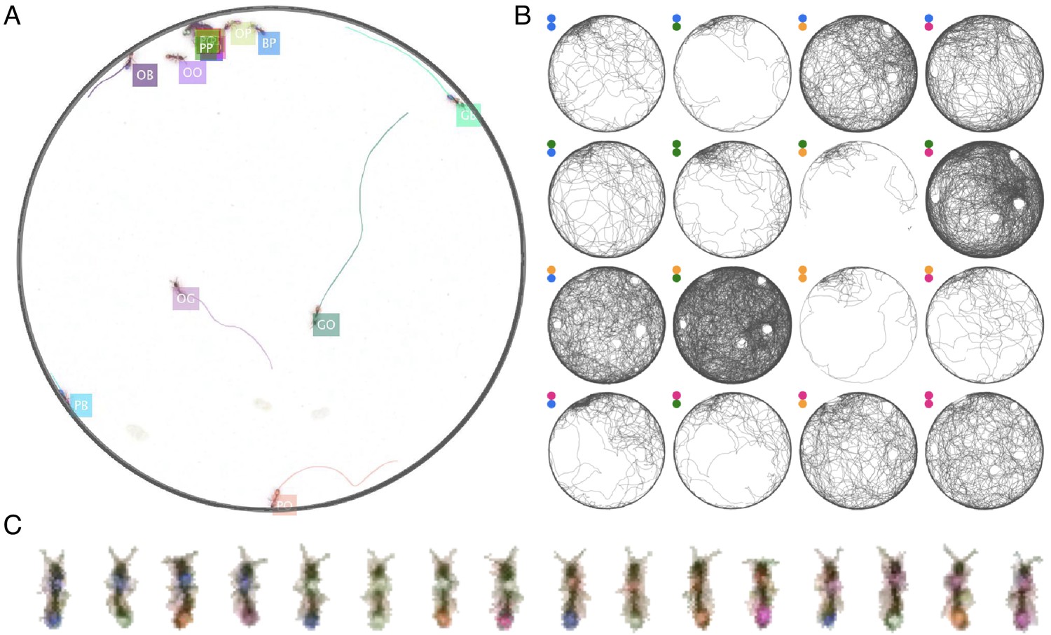
Example of anTraX tracking output, based on the J16 dataset.
In this experiment, the ants are freely behaving in a closed arena that contains the nest (the densely populated area on the top left) and exploring ants. A short annotated clip from the tracked dataset is given as Figure 3—video 1. Tracking outputs and annotated videos of all datasets are also given in the supplementary figures and videos of this figure. (A) A labeled frame (background subtracted), showing the location of each ant in the colony, as well as a ‘tail’ of the last 10 s of trajectory. Ants that are individually segmented have precise locations. The ants clustered together have approximate locations. Labels indicate the color tag combination of the ant (e.g. ‘BG’ indicates a blue thorax tag and a green abdomen tag; colors are blue (B), green (G), orange (O), and pink (P)). (B) Individual trajectories for each ant in the colony, based on 1 hr of recording. (C) A cropped image of each ant from the video.
Figure 3—figure supplement 1
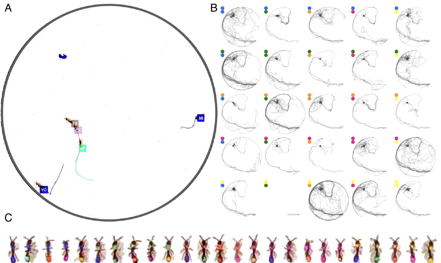
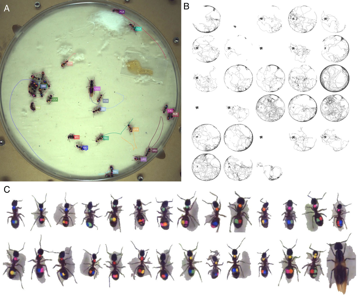
Tracking the V25 dataset with 25 O. biroi ants.
The figure follows the same format as Figure 3.
Figure 3—figure supplement 2
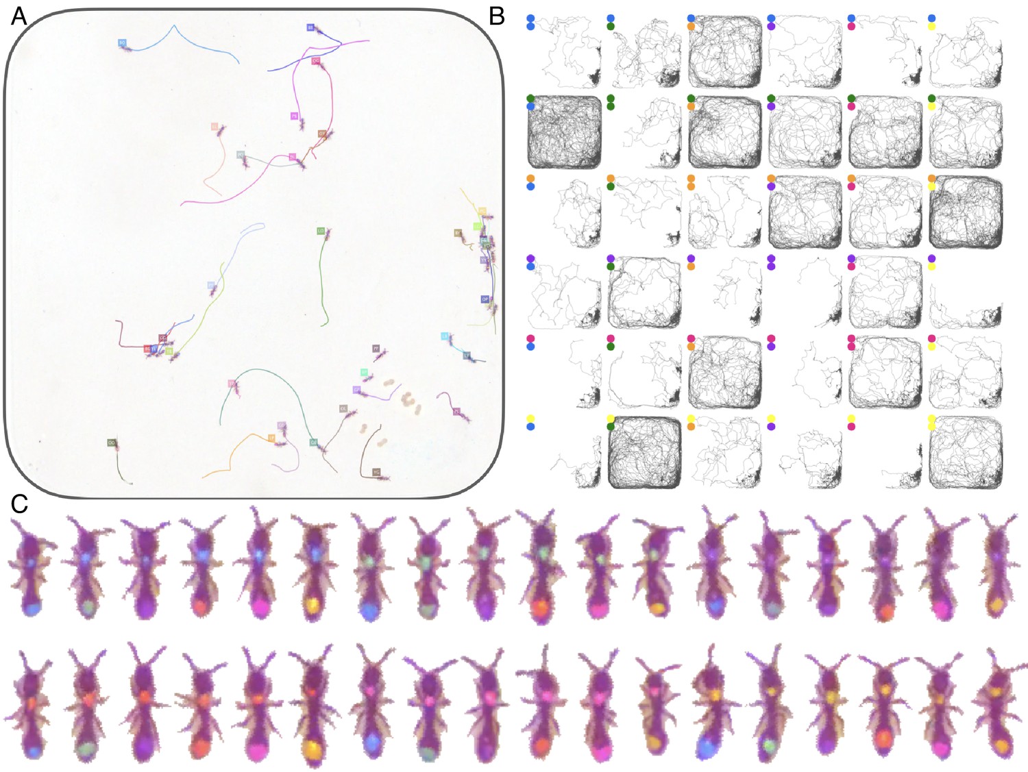
Tracking the A36 dataset with 36 O. biroi ants.
The figure follows the same format as Figure 3.
Figure 3—figure supplement 3

Tracking the T10 dataset with 10 T. nylanderi ants.
The figure follows the same format as Figure 3.
Figure 3—figure supplement 4
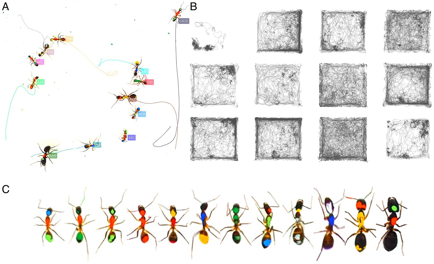
Tracking the T10 dataset with 12 C. fellah ants.
The figure follows the same format as Figure 3.
Figure 3—figure supplement 5
Tracking the C32 dataset with 28 Camponotus spec. ants, including an unmarked winged queen.
The figure follows the same format as Figure 3.
Figure 3—figure supplement 6
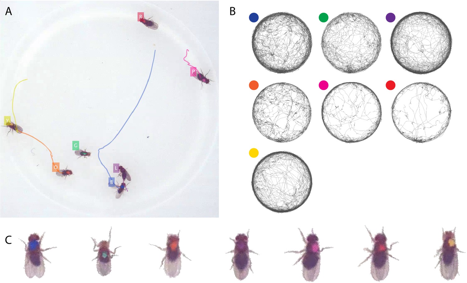
Tracking the D7 dataset with seven D. melanogaster fruit flies.
The figure follows the same format as Figure 3.
Figure 3—figure supplement 7

Tracking the D16 dataset with 16 D. melanogaster fruit flies.
The figure follows the same format as Figure 3.
Figure 3—figure supplement 8
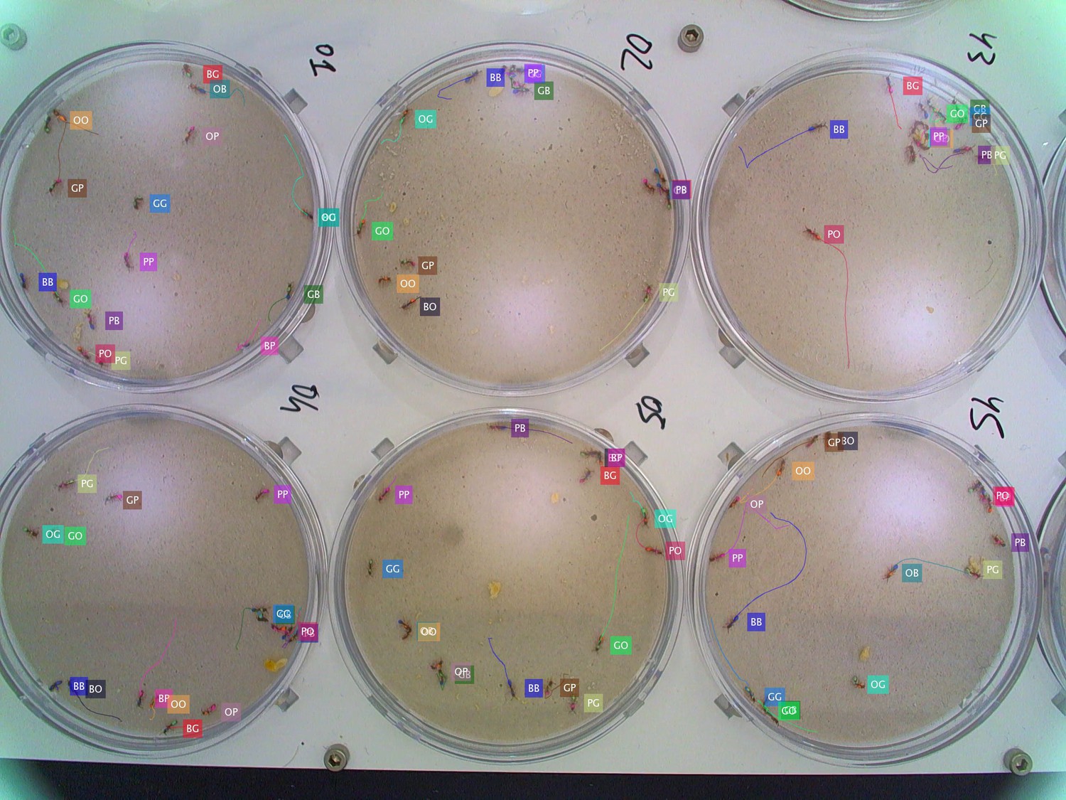
Tracking the G6 × 16 dataset with six colonies of 16 O. biroi ants each recorded and tracked in parallel.
Figure 3—video 1
An annotated tracking video clip from dataset J16.
Figure 3—video 2
An annotated tracking video clip from dataset V25.
Figure 3—video 3
An annotated tracking video clip from dataset A36.
Figure 3—video 4
An annotated tracking video clip from dataset T10.
Figure 3—video 5
An annotated tracking video clip from dataset C12.
Figure 3—video 6
An annotated tracking video clip from dataset C32.
Figure 3—video 7
An annotated tracking video clip from dataset D7.
Figure 3—video 8
An annotated tracking video clip from dataset D16.
Figure 3—video 9
An annotated tracking video clip from dataset G6 × 16.
Figure 4 with 3 supplements
Tracking performance.
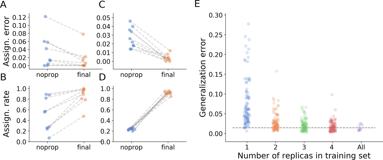
(A) Contribution of graph inference to reduction of assignment error. The graph compares the assignment error in the benchmark datasets, defined as the rate of assigning wrong IDs to blobs across all IDs and frames in the experiment, and estimated as explained in the main text, before the graph propagation step of the algorithm (blue circles, ‘noprop’ category) and after the graph propagation step (orange circles, ‘final’ category). (B) Contribution of graph inference to increased assignment rate (the ratio of assignments made by anTraX to the total number of assignments possible in the experiment) in the benchmark datasets. The graph compares the assignment rate, as defined in the main text, before and after the graph propagation step (same depiction as in A). The performance measures for all benchmark datasets are reported in Table 2 and Figure 4—source data 1. (C–D) Same as in A and B, calculated for a large-scale dataset described in the text (10 colonies of 16 ants, recorded over 14 days). The performance measures for all replicas are reported in Figure 4—source data 2. (E) Generalizability of the blob classifier. Each point in categories 1–4 represents the generalization error of one classifier (trained with examples from number of replicas corresponding to its category) on data from one replica that was not used for its training. The replicas were recorded under similar conditions, but using different ants, different cameras, and different experimental setups. For classifiers trained on more than one replica, the combinations of replicas were randomly chosen, while maintaining the constraint that each replica is tested against the same number of classifiers in each condition. In the category ‘All’, the points depict the validation error of the full classifier, trained on data from the 10 replicas. All classifiers were trained with the same network architecture, started training from a scratch model, and were trained until saturation. The dashed line represents the mean validation error for the full classifier. The list of errors for all trained classifiers are given in Figure 4—source data 3.
-
Figure 4—source data 1
A table of performance measures, as defined in the main text, for the benchmark datasets.
The data in this file were used to plot Figure 4A–B and Figure 4—figure supplement 1A,C, and are referenced in Table 2.
- https://cdn.elifesciences.org/articles/58145/elife-58145-fig4-data1-v1.csv
-
Figure 4—source data 2
A table of performance measures, as defined in the main text, for the 10-replica experiment described in the main text.
The data in this file were used to plot Figure 4C–D and Figure 4—figure supplement 1B,D.
- https://cdn.elifesciences.org/articles/58145/elife-58145-fig4-data2-v1.csv
-
Figure 4—source data 3
A table of generalization errors for all classifiers, as described in the caption of Figure 4E.
The data in this file were used to plot Figure 4E.
- https://cdn.elifesciences.org/articles/58145/elife-58145-fig4-data3-v1.csv
Figure 4—figure supplement 1
Error comparison between assignments made by direct classification and assignments made by the propagation algorithm.
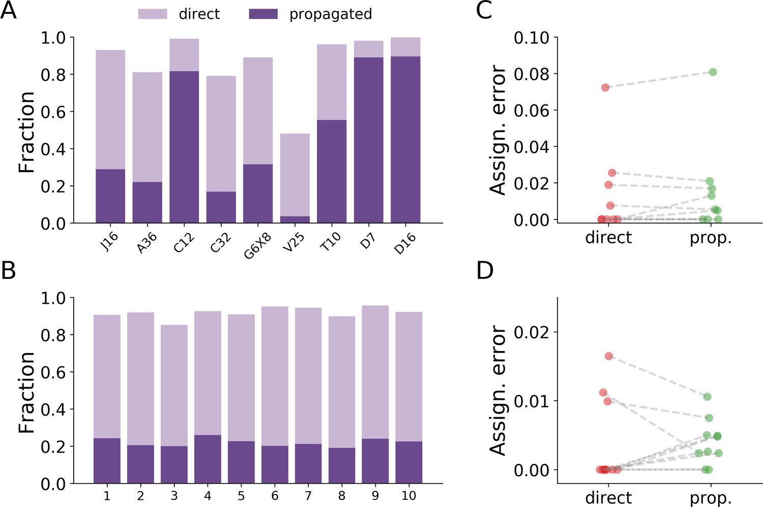
(A) The relative fraction of assignment types for the benchmark datasets. Some datasets have only a small proportion of their assignments made by direct classification (e.g. dataset V25), while datasets with low interaction rates have most of their assignments made by direct classification (e.g. the Drosophila datasets D7 and D16). The two types of assignments add up to the total assignment rates as reported in Table 2. (B) The relative fraction of assignment types for the large-scale dataset described in the text (10 colonies of 16 ants each, recorded over 14 days). Here, the variability between the replicas is much reduced compared to the variability between the benchmark datasets in A. (C) The error in assignments via direct classification vs. propagation for the benchmark datasets. The errors were estimated by the same procedure used to estimate the total assignment error in Figure 4. The set of 500 random points was split according to the type of assignment, and the error was estimated by taking the relative number of incorrect assignments. No clear effect is observed between the groups (paired t-test, p=0.338). (D) The error in assignments via direct classification vs. propagation for the experiment in panel B, estimated as in C. No clear effect is observed between the groups (paired t-test, p=0.866). The low variability in the relative fraction of each assignment type between the replicas in this experiment also allows us to compare the total error, by pooling all 5000 validation points across all replicas. The total estimated error of assignments made by the classifier is 0.0039, with a 95% confidence interval of 0.0011–0.102, while the total estimated error of assignments made by the propagation algorithm is 0.0041, with a 95% confidence interval of 0.0025–0.0068. Overall, these results show that there is no systematic dependency of the assignment error on the step of the algorithm responsible for the assignment. Data for all plots in this figure are given in Figure 4—source data 1 and Figure 4—source data 2.
Figure 4—figure supplement 2
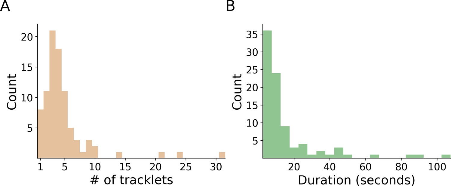
Propagation of errors.
In total, we detected 88 assignment errors in the validation procedure across all experiments. For each of these errors, we manually extracted the length of the erroneous segment, both in terms of number of tracklets (A) and time (B). Both histograms show that the algorithm is robust against error propagation, and successfully terminates the propagation after a small number of propagation steps. Checking the instances where the error was propagated for more than four steps showed that, in each case, the reason was that more than one incorrect classification existed in the erroneous segment. The raw data for the histograms are given in Figure 4—figure supplement 2—source data 1 and Figure 4—figure supplement 2—source data 2.
-
Figure 4—figure supplement 2—source data 1
The count data for the histogram plotted in Figure 4—figure supplement 2A.
- https://cdn.elifesciences.org/articles/58145/elife-58145-fig4-figsupp2-data1-v1.csv
-
Figure 4—figure supplement 2—source data 2
The count data for the histogram plotted in Figure 4—figure supplement 2B.
- https://cdn.elifesciences.org/articles/58145/elife-58145-fig4-figsupp2-data2-v1.csv
Figure 4—figure supplement 3
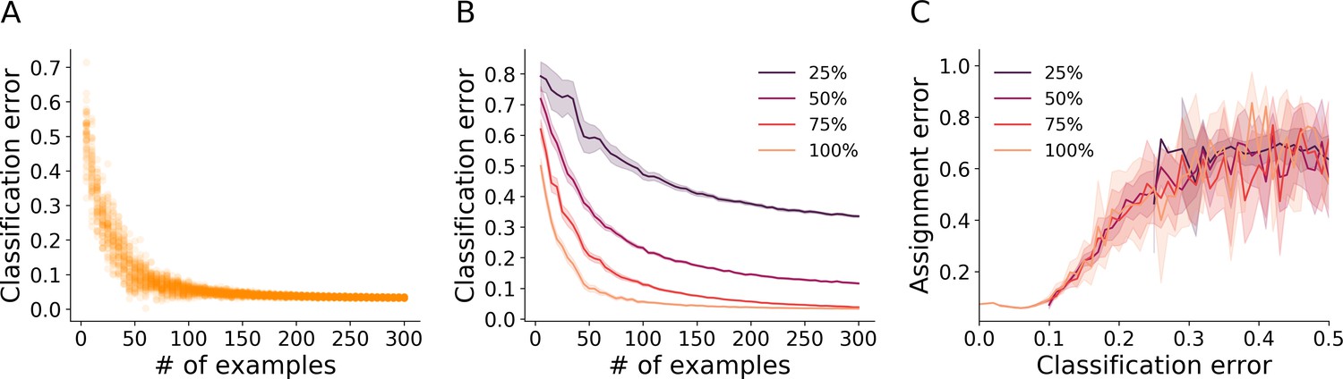
Classification and assignment errors.
(A) Cross-validation error of the blob classifier as a function of the number of examples per class in the training set. Each point represents an iteration of training/validation on a reduced labeled example set sampled randomly from the full example set of benchmark dataset A36 (36 O. biroi ants marked with two color dots each, see Table 1). For each value tested for the number of examples, 50 independent realizations of an example set of that size were sampled from the full example set. For each of these sampled example sets, a classifier was trained with 80% of the sampled examples, and its error was estimated on the remainder of the examples. (B) The procedure in A was repeated, but with the resolution of the example images reduced before training to 75%, 50% and 25% of the original size. Depicted are the mean and 95% confidence intervals of the cross-validation errors of the trained classifiers. (C) We used each classifier trained in B to classify the tracklets of 1 hr worth of tracking data from dataset A36, and then ran the propagation step of the algorithm. We estimated the resulting assignment error relative to a manually annotated set of validation points sampled randomly. We then plotted (mean and 95% confidence interval bands) the assignment error as a function of the classifier’s cross validation error. The graph shows that below a certain classification accuracy (around 90% in this case), the tracking error climbs rapidly. Moreover, the data of the classifiers from all image resolutions collapse onto a single curve, suggesting that the error of the classifier is the sole predictor of the final assignment error, irrespective of whether it is due to an insufficiently large training set or poor image quality.
Figure 5 with 3 supplements
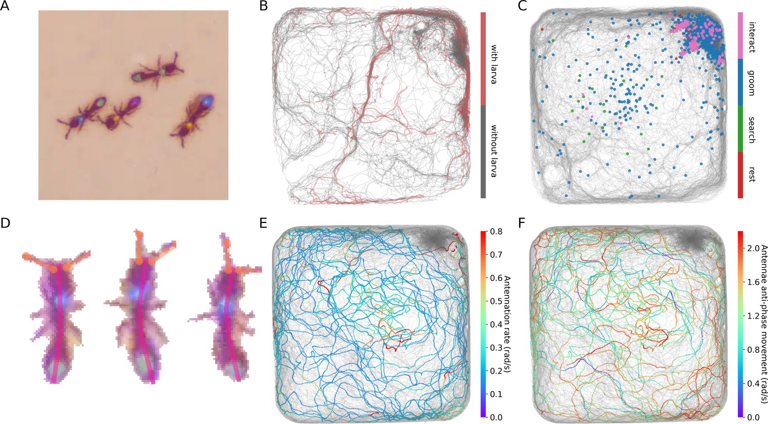
Interfacing anTraX with third party behavioral analysis packages for augmenting tracking data.
(A) Ants carrying a larva while they move (green/green and yellow/blue) can be difficult to distinguish from ants not carrying larvae (blue/green and yellow/purple), even for a human observer. Figure 5—video 1 shows examples for ants walking with and without a larva. (B) However, using labeled examples to train a classifier, JAABA can reliably distinguish ants walking while carrying a larva from ants walking without one from anTraX tracking output. Shown here is a 30 min segment from the A36 dataset, where trajectories classified by JAABA as ants carrying a larva are plotted in red on the background of all other tracks (in gray). (C) Classifying stops using JAABA. The plot shows a 60 min segment from the A36 experiment, where all stops longer than 2 s are marked with a colored dot. The stops are classified into four categories: rest (red), local search (green), self-grooming (blue), and object-interaction (e.g. with a food item; pink). Figure 5—video 2 shows examples of stops from all types. (D) Applying a simple DeepLabCut model to track the ants’ antennae and main body axes, shown on segmented ant images from dataset A36. Figure 5—video 3 shows an animated tracking of all ants in the colony. (E–F) Using the results from DeepLabCut to track the behavior of an ant along its trajectory. A one-hour trajectory of one ant from dataset A36 is shown on the background of the tracks of all other ants in the colony in that period (in gray). In E, the focal trajectory is colored according to the total rate of antennal movement (measured in angular velocity units rad/s). In F, the focal trajectory is colored according to how much the antennae move in-phase or anti-phase (measured in angular velocity units rad/s). Together, these panels show the behavioral variability in antennal movement patterns.
Figure 5—video 1
Examples of short video clips from dataset A36 in which some ants walk carrying a larva, while others walk without a larva.
Clips like these were used to train the JAABA classifier in Figure 5B.
Figure 5—video 2
Examples of short video clips from dataset A36 showing the four types of stop behavior.
Clips like these were used to train the JAABA classifier in Figure 5C.
Figure 5—video 3
Pose-tracking of all ants in dataset A36 using anTraX in combination with DeepLabCut.
Appendix 1—figure 1
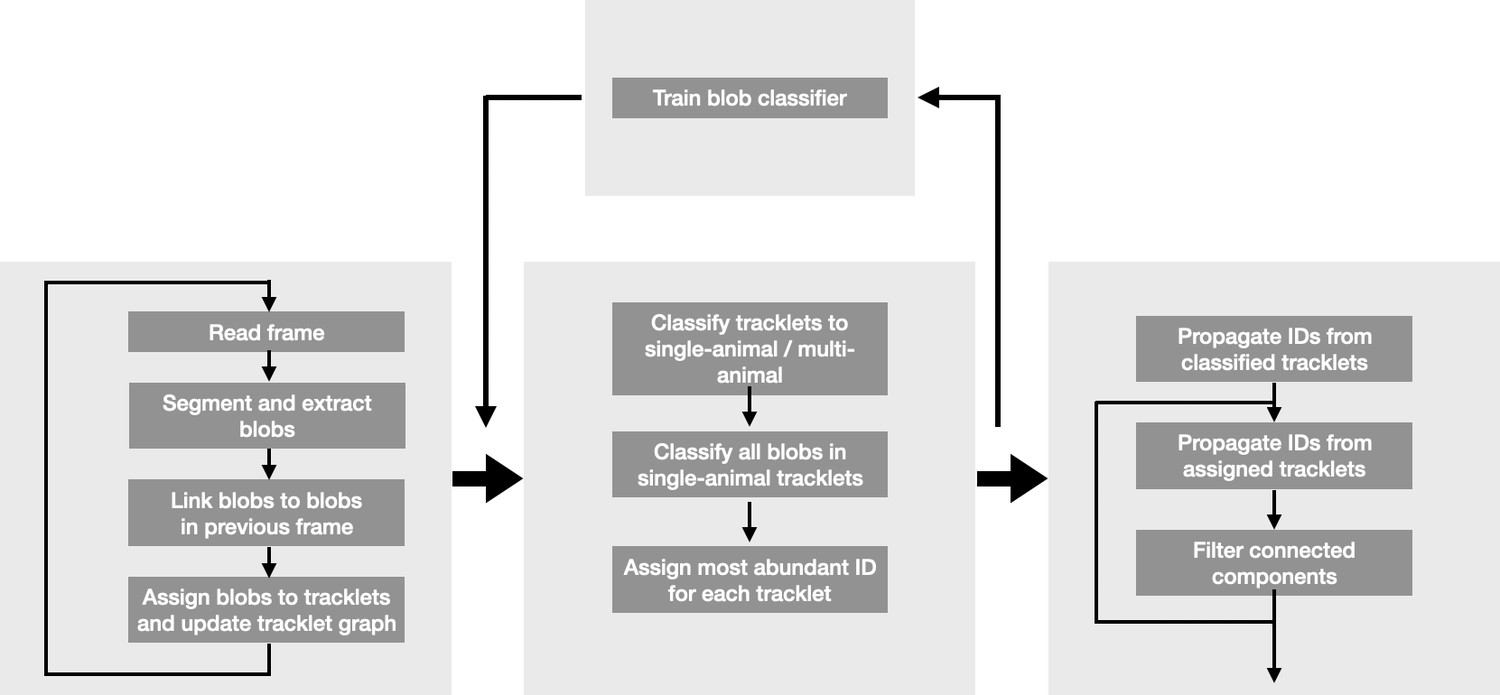
Flow diagram of the anTraX algorithm.
Appendix 1—figure 2
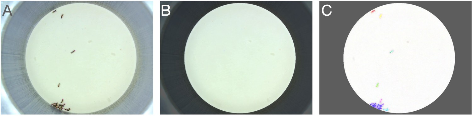
Background creation.
(A) An example raw frame. (B) A background frame generated using a median function. Regions outside the ROI mask are dimmed. (C) Full segmented frame.
Appendix 1—figure 3

Image segmentation.
(A) Raw image. (B) Background subtracted grayscale image. (C) Unfiltered binary image. (D) Final segmented image after morphological operations and blob filtering. Each separate blob is shown in a different color.
Appendix 1—figure 4
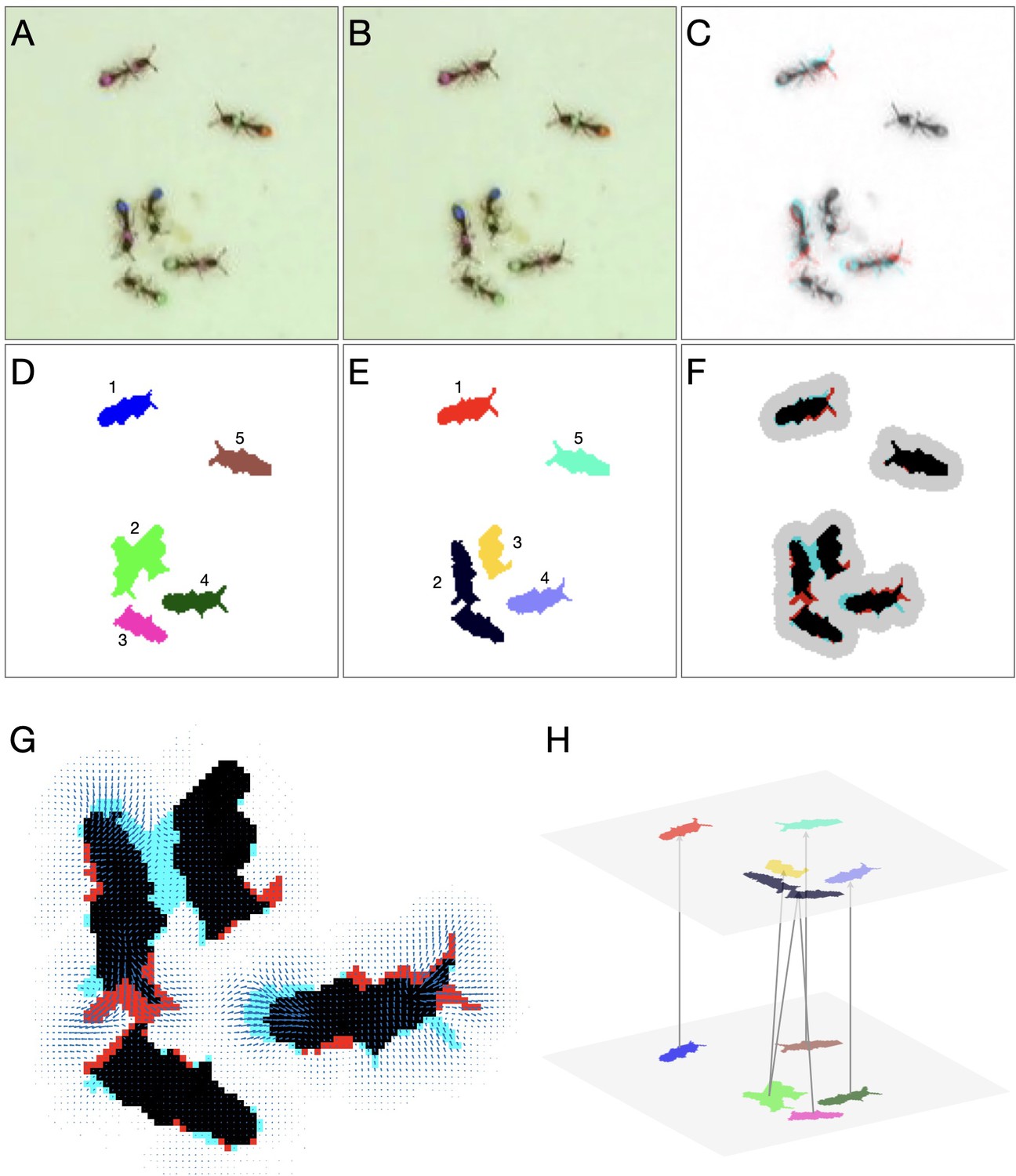
Detailed linking example.
(A–B) Raw images of the first and second frame, respectively. (C) Color blend of the frames, showing the displacement of the ants between frames. (D–E) Segmentation of the first and second frame, respectively. (F) Segmentation blend. Also shown is the clustering of the blobs into linking problems (gray background). The two upper problems are trivial, and no assignment algorithm is required. The problem at the bottom will be solved using optical flow. (G) Optical flow for the bottom problem in F. Arrows represent the estimated translation of the pixels. (H) Final linking between the blobs based on optical flow.
Appendix 1—figure 5
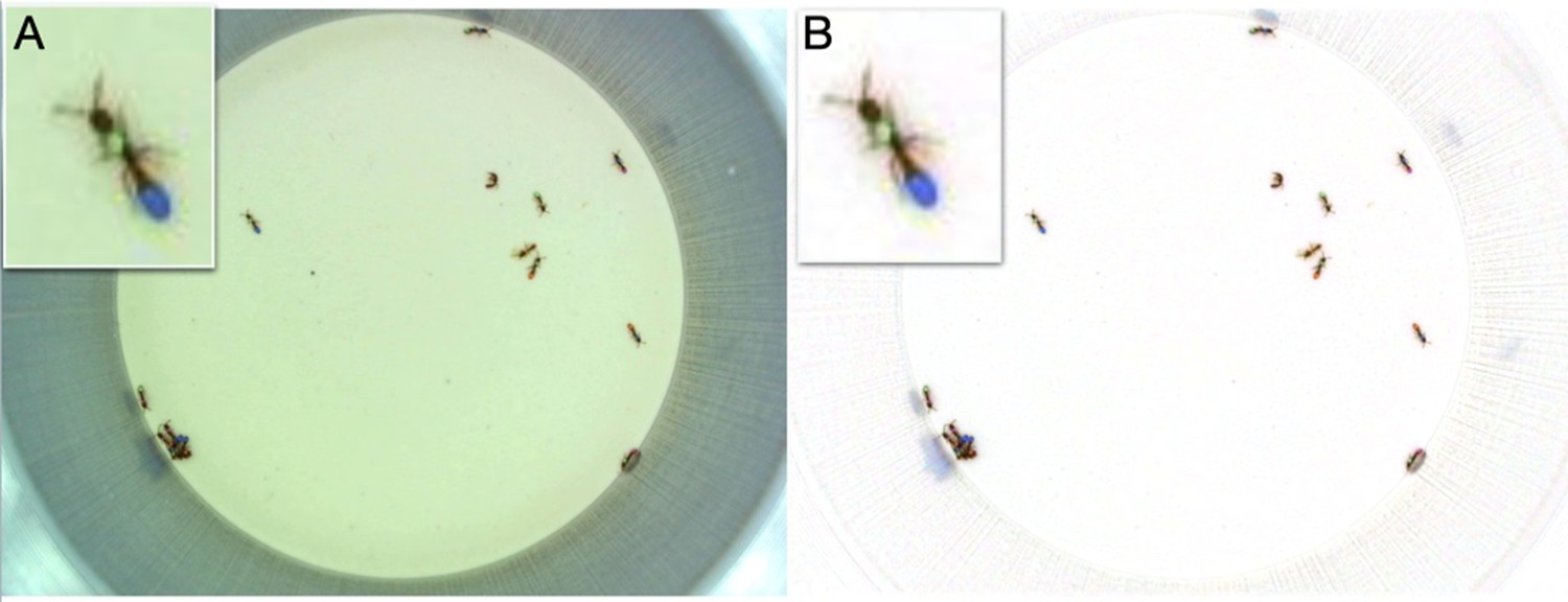
Color correction.
(A) The original frame. (B) The color corrected frame. Insets show a zoomed in view of a focal ant. The color correction removes the green bias in the original frame and enhances the color segmentation.
Appendix 1—figure 6
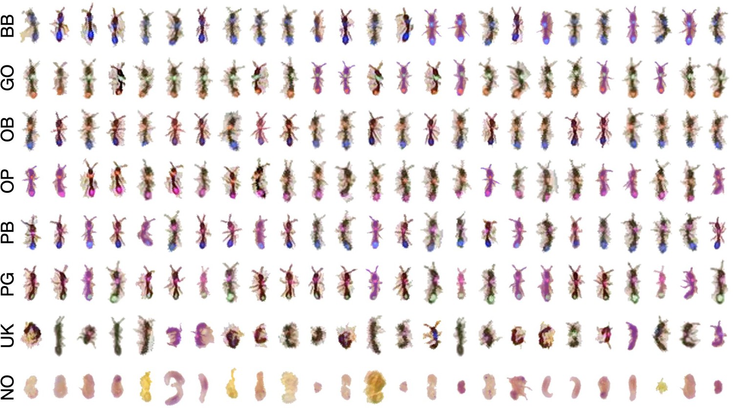
An example subset from a training set.
Shown are examples from six ant IDs with a total of four tag colors. The UK label represents ant images that are not classifiable to the human eye. The NO label represents segmented objects that are not ants (food items, larvae, etc). To allow the classifier to generalize well, it is important that the variability of the training set captures the variability in the experiment, and includes images of ants in various poses, lighting conditions, and across experimental replicates.
Appendix 1—figure 7
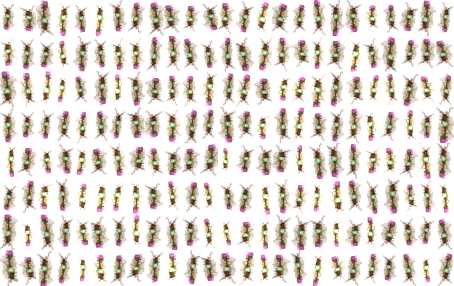
Dataset augmentation using TensorFlow’s intrinsic mechanism for image transformation on a single example image to generate a larger training dataset.
Appendix 1—figure 8
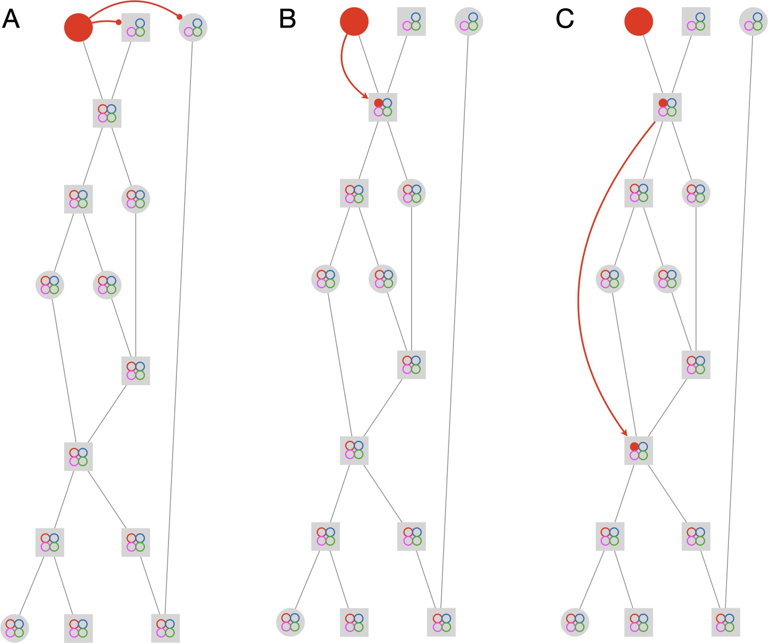
Propagation rules.
The figure depicts the first three steps in solving an example graph. The graph has 15 tracklets and 4 IDs. Circular nodes mark single-animal tracklets, while square nodes mark multi-animal tracklets. The colored circles inside the nodes mark the current assignments of the node. Empty circles indicate possible assignments, and full circles indicate actual assignments. The full solution of the example is given in Figure 2—video 1. (A) Negative horizontal propagation. (B) Positive vertical propagation. (C) Positive topological propagation.
Appendix 1—figure 9
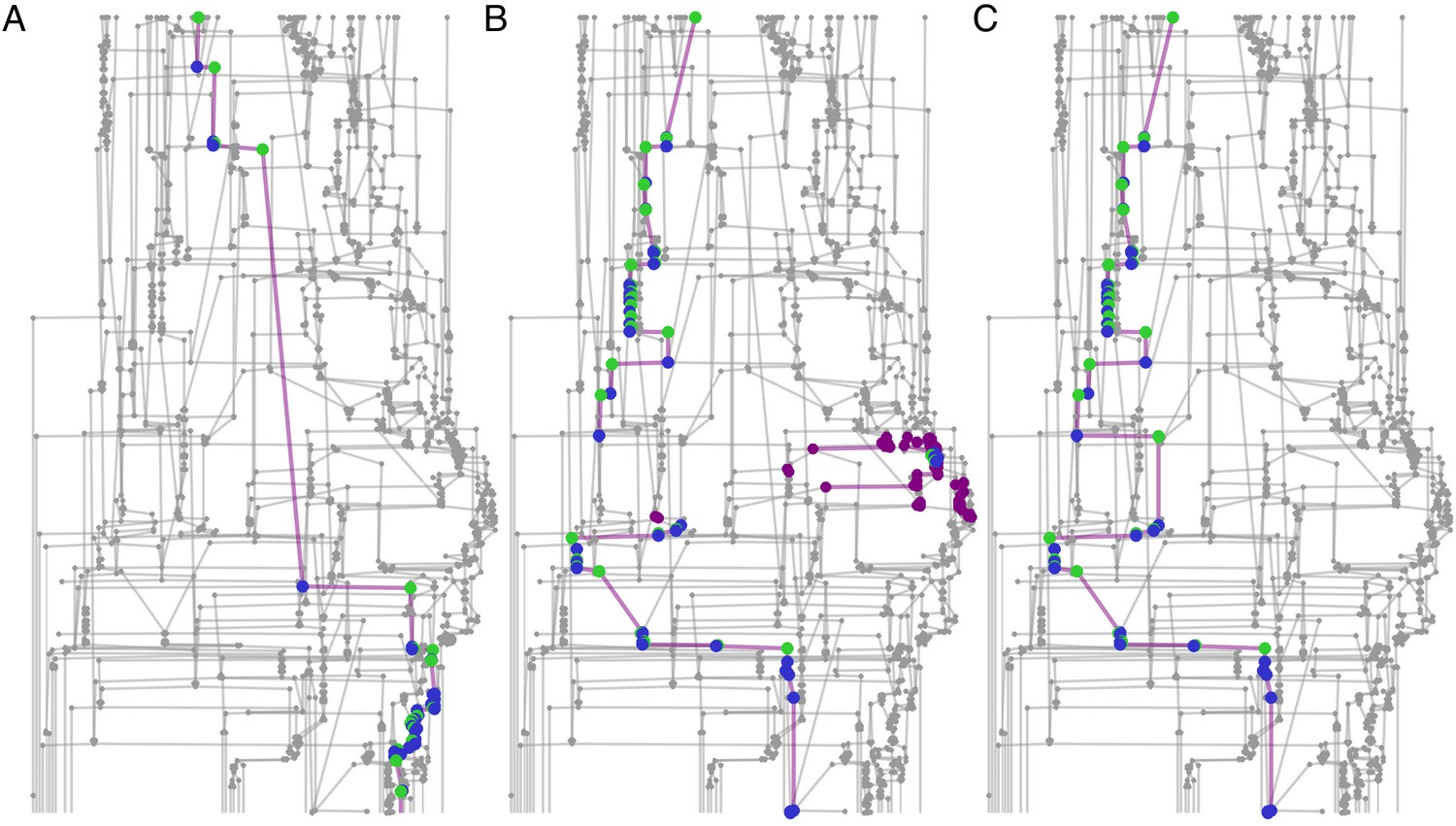
Connected component filtering.
An example from a 10-min tracklet graph. Green nodes are those assigned by the classifier, blue nodes are assigned by the propagation algorithm, and purple nodes are ambiguous (‘possible’ but not ‘assigned’). (A) A focal ant subgraph in which graph assignment propagation was consistent and did not result in contradictions. (B) A subgraph for a different focal ant in the same graph, for which the classifier made an incorrect assignment. As a consequence, the subgraph is fractured into a few connected components. (C) The subgraph of the same focal ant as in B, following the connected component filtering step and a second round of assignment propagations. The erroneous component was filtered, and the algorithm was able to complete the ID path through the graph.
Tables
Table 1
Summary description of the benchmark datasets.
All raw videos and parameters of the respective tracking session are available for download (Gal et al., 2020b).
| Dataset | Species | #Animals | #Colors | #Tags | Open* ROI | Duration (hr) | Camera | FPS | Image size (pixels) | Resolution (pixels/mm) |
|---|---|---|---|---|---|---|---|---|---|---|
| J16 | Ooceraea biroi | 16 | 4 | 2 | No | 24 | Logitech C910 | 10 | 960 × 720 | 10 |
| A36 | Ooceraea biroi | 36 | 6 | 2 | No | 24 | PointGrey Flea3 12MP | 10 | 3000 × 3000 | 25 |
| C12 | Camponotus fellah | 12 | 7 | 3 | No | 6 | Logitech C910 | 10 | 2592 × 1980 | 17 |
| C32 | Camponotus sp. | 28 | 6 | 3 | No | 24 | PointGrey Flea3 12MP | 10 | 2496 × 2500 | 13 |
| G6 × 16 | Ooceraea biroi | 6 × 16† | 3 | 2 | No | 1.33 | Logitech C910 | 10 | 2592 × 1980 | 17 |
| V25 | Ooceraea biroi | 25 | 5 | 2 | Yes | 3 | Logitech C910 | 10 | 2592 × 1980 | 17 |
| T10 | Temnothorax nylanderi | 10 | 5 | 4 | No | 6 | Logitech C910 | 10 | 2592 × 1980 | 17 |
| D7 | Drosophila melanogaster | 7 | 7 | 1 | No | 3 | PointGrey Flea3 12MP | 18 | 1056 × 1050 | 26 |
| D16 | Drosophila melanogaster | 16 | 4 | 2 | No | 5 | PointGrey Flea3 12MP | 18 | 1200 × 1200 | 16 |
-
ROI: region of interest; FPS: frames per second. *Whether or not the ants can leave the tracked region. †Dataset G6 × 8 is derived from six replicate colonies with eight ants each.
Table 2
Summary of tracking performance measures for the benchmark datasets using anTraX.
Assignment rate is defined as the proportion of all data points (the number of individuals times the number of frames) in which a blob assignment was made. In cases of closed boundary regions of interest (ROIs; in which the tracked animals cannot leave the tracked region) this measure is in the range of 0–1. In cases of open boundary ROIs (marked with asterisks; e.g., dataset V25), the upper boundary is lower, reflecting the proportion of time the ants are present in the ROI. The assignment error is an estimation of the proportion of wrong assignments (i.e. an ant ID was assigned to a blob the respective ant is not present in). As explained in the text, the estimation is done by sequentially presenting the user with a sequence of randomly sampled assignments from the dataset and measuring the proportion of assignments deemed ‘incorrect’ by the observer, relative to the sum of all ‘correct’ and ‘incorrect’ assignments. To calculate the error rates reported in the table, the presentation sequence continued until exactly 500 assignments were marked as ‘correct’ or ‘incorrect’, ignoring cases with the third response ‘can’t say’. A 95% confidence interval of the error according to the Clopper-Pearson method for binomial proportions is also reported in the table. To quantify the contribution of using graph propagation in the tracking algorithm, the analysis was repeated ignoring assignments made during the graph propagation step, and the results are reported here for comparison. A graphical summary of the performance measures is shown in Figure 4A–B.
| Without graph propagation | With graph propagation | |||||
|---|---|---|---|---|---|---|
| Dataset | Assignment rate | Assignment error | Assignment error 95% CI | Assignment rate | Assignment error | Assignment error 95% CI |
| J16 | 0.28 | 0.012 | 0.0044–0.026 | 0.93 | 0 | 0–0.0074 |
| A36 | 0.24 | 0.014 | 0.0056–0.0286 | 0.81 | 0.006 | 0.0012–0.0174 |
| C12 | 0.82 | 0 | 0–0.0074 | 0.99 | 0 | 0–0.0074 |
| C32 | 0.26 | 0.042 | 0.0262–0.0635 | 0.79 | 0.022 | 0.011–0.039 |
| G6 × 16 | 0.57 | 0.122 | 0.0946–0.154 | 0.89 | 0.078 | 0.056–0.105 |
| V25 | 0.07* | 0.058 | 0.0392–0.0822 | 0.48* | 0.012 | 0.0044–0.026 |
| T10 | 0.56 | 0.06 | 0.041–0.0845 | 0.96 | 0.018 | 0.0083–0.339 |
| D7 | 0.88 | 0 | 0–0.0074 | 0.98 | 0 | 0–0.0074 |
| D16 | 0.89 | 0.004 | 0.0005–0.0144 | 0.997 | 0 | 0–0.0074 |
Additional files
Download links
A two-part list of links to download the article, or parts of the article, in various formats.
Downloads (link to download the article as PDF)
Open citations (links to open the citations from this article in various online reference manager services)
Cite this article (links to download the citations from this article in formats compatible with various reference manager tools)
anTraX, a software package for high-throughput video tracking of color-tagged insects
eLife 9:e58145.
https://doi.org/10.7554/eLife.58145


