Minimally dependent activity subspaces for working memory and motor preparation in the lateral prefrontal cortex
- Institute of Molecular and Cell Biology, A*STAR, Singapore
- The N1 Institute for Health, National University of Singapore (NUS), Singapore
- Department of Psychology, NUS, Singapore
- Innovation and Design Programme, Faculty of Engineering, NUS, Singapore
Figures
Figure 1
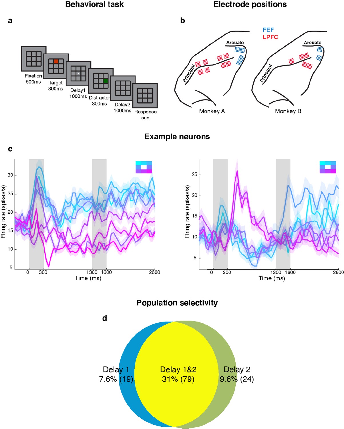
Experimental design and responses of example neurons.
(a) Behavioral task: Each trial began when the animal fixated on a fixation spot at the center of the screen. The animal was required to maintain fixation throughout the trial until the fixation spot disappeared. A target (red square) was presented for 300 ms followed by a 1000 ms delay period (Delay 1). A distractor (green square) was then presented for 300 ms in a random location that was different from the target location and was followed by a second delay of 1000 ms (Delay 2). After Delay 2, the fixation spot disappeared, which was the Go cue for the animal to report, using an eye movement, the location of the target. (b) Implant locations of 16-channel and 32-channel electrode arrays (with electrode lengths ranging from 5.5 mm closer to the sulci, to 1 mm further from the sulci) in the LPFC (red dots) and the FEF (blue dots) in the two animals. Analyses were carried out only on LPFC data. (c) Peristimulus time histograms (PSTH) for two single neurons in the LPFC. Time 0 marks the onset of target presentation; responses to the different target locations are color-coded according to the legend shown in the top right; the colored regions surrounding each line indicates the standard error. (d) Venn diagram showing the number of LPFC neurons selective in Delay 1, in Delay 2, and their overlap. Target selectivity was tested using one-way ANOVA (p < 0.05) with spike counts averaged during 800–1300 ms for Delay 1 and 2100–2600 ms for Delay 2.
Figure 2 with 7 supplements
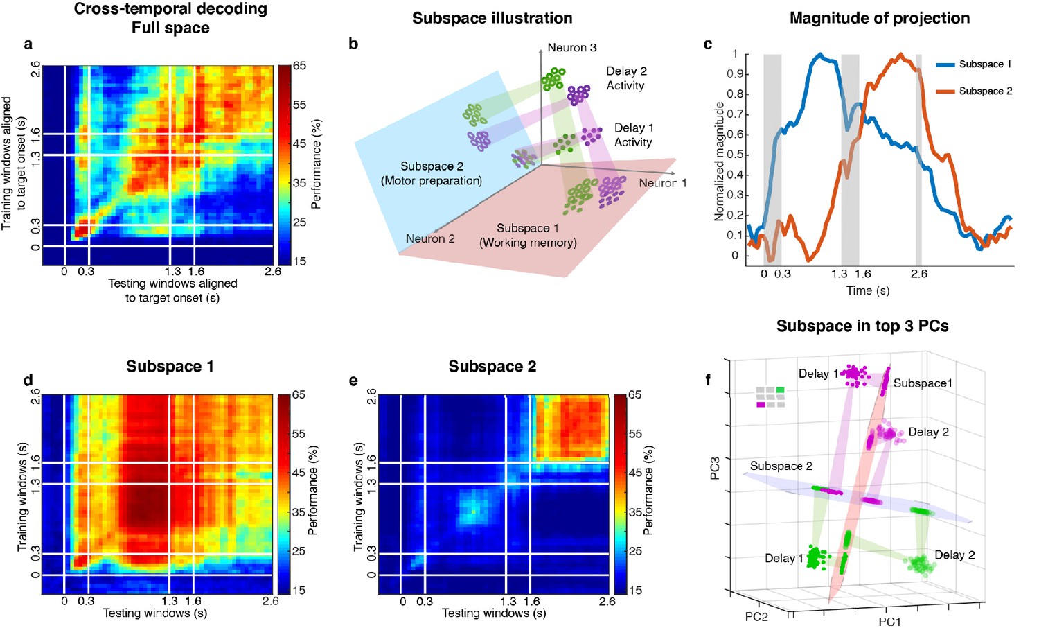
Code morphing, and two minimally dependent subspaces.
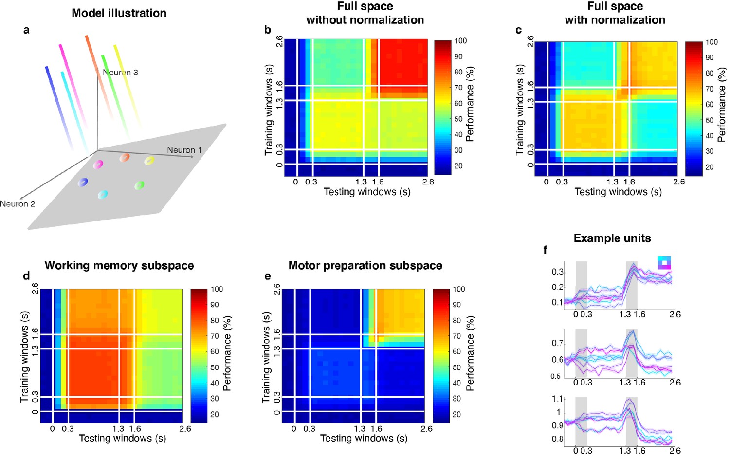
(a) Heat map showing the cross-temporal population-decoding performance in the LPFC. White lines indicate target presentation (0–0.3 s), distractor presentation (1.3–1.6 s), and cue onset (2.6 s). (b) Schematic illustration of the projection of the full-space activity into Subspace 1 and Subspace 2. Delay 1 activity (purple and green filled circles) projected into the Subspace 1 would cluster according to target location (filled circles in the red subspace), and because this was a stable subspace, the Delay 2 activity for each target location (purple and green unfilled circles) would overlap with those for Delay 1 (open circles in the red subspace). In Subspace 2, Delay 1 activity would not cluster according to location (filled circles in the blue subspace), and the clustering by location would emerge only from the Delay 2 activity (open circles in the blue subspace) after the emergence of the new information. (c) We projected the trial-averaged full-space population activity for each time bin across the whole trial into Subspace 1 and Subspace 2 and calculated the magnitude of the projections. For each subspace, the magnitude was normalized to have a maximum value of 1. The projections into Subspace 1 and Subspace 2 exhibited different temporal profiles. (d) Cross-temporal decoding performance after projecting full-space activity into Subspace 1. (e) Cross-temporal decoding performance after projecting full-space activity into Subspace 2. (f) Projection of single-trial activity for two target locations (actual locations shown in the upper left corner) onto the first three principal components. Delay 1 is depicted as closed circles, and Delay 2 as open circles. Re-projections into the Subspace 1 (red plane) and Subspace 2 (blue plane) are shown and guided by projection cones (green and purple cones connecting the PCA projections into the subspace re-projections).
Figure 2—figure supplement 1
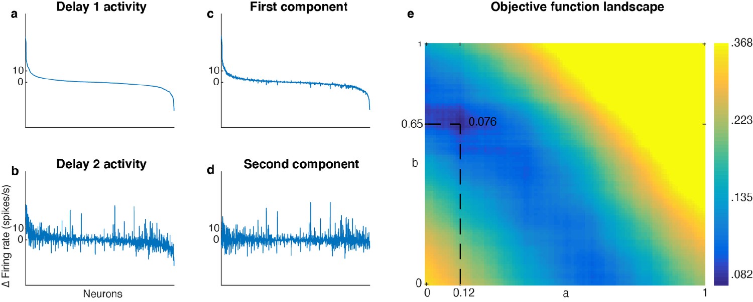
Unmixed population activity between Delay 1 and Delay 2.
(a) Delay 1 population activity for all seven target locations sorted according to firing rate. The x-axis has 1582 points (226 cells x seven locations). Each neuron’s firing rate for the last 500 ms of Delay 1 on each trial was averaged across time, before being averaged across trials in each location. This was then subtracted by the average baseline firing rate (averaged across 300 ms prior to target presentation before averaging across trials). The neurons were sorted in descending order by the Delay 1 activity (a to d).( b) Delay 2 population activity, significantly correlated with Delay 1 activity (r = 0.69, p < 0.001, mutual information = 0.33 bits). (c) The unmixed Element 1. (d) The unmixed Element 2, has minimal mutual information with Element 1 (r = 0.017, p = 0.5, mutual information = 0.076 bits). (e) Heatmap showing the landscape of the objective function for unmixing Delay 1 and Delay 2 activity. There was a global minimum when a = 0.12 and b = 0.65.
Figure 2—figure supplement 2
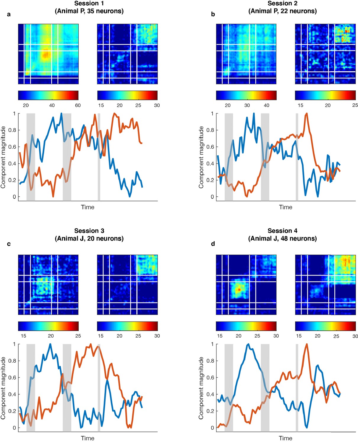
Single-session subspace identification.
For each single session in the two monkeys, we applied the unmixing method to the activity of simultaneously recorded neurons rather than a pseudo-population. (a) Top left, cross-temporal decoding performed in the working memory subspace identified from 35 simultaneously recorded neurons. DM11 = 41.0 ± 1.7% (trained and tested in Delay 1 in the working memory subspace), DM22 = 31.1 ± 1.8% (trained and tested in Delay 2 in the working memory subspace). Top right, cross-temporal decoding performed in the motor preparation subspace identified from the same population of neurons. DP11 = 16.5 ± 1.6%, DP22 = 20.8 ± 1.9%. Bottom, projection magnitude of full-space activity into each subspace (refer to Figure 1d). (b), Same as (a), but for another single session from Animal P. DM11 = 26.2 ± 1.4%, DM22 = 23.8 ± 1.2%, DP11 = 15.1 ± 1.2%, DP22 = 19.0 ± 1.1%. (c), Same as (a), but for a single session from Animal J. DM11 = 17.8 ± 0.9%, DM22 = 14.6 ± 0.7%, DP11 = 15.0 ± 0.9%, DP22 = 19.8 ± 0.8%. (d Same as c) but for another single session from Animal J. DM11 = 21.2 ± 1.0%, DM22 = 17.2 ± 0.9%, DP11 = 16.0 ± 1.1%, DP22 = 23.3 ± 0.9%. The single-session results showed higher decoding performance in Delay 1 than in Delay 2 in the working memory subspace, higher decoding performance in Delay 2 than in Delay 1 in the motor preparation subspace, and the projection magnitude into the two subspaces showed different temporal profiles, consistent with the results obtained from the pseudo-population analysis in Figure 1. This analysis validates the existence of working memory and motor preparation subspaces in simultaneously recorded neurons in different animals.
Figure 2—figure supplement 3
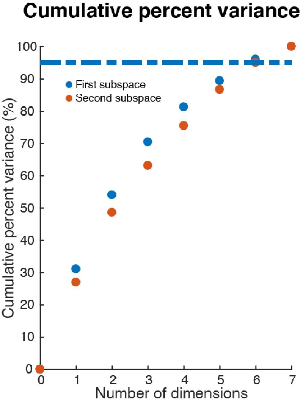
Effective dimension of full-space data in the subspaces.
We projected single-trial full-space activity (250 pseudo-trials each location, seven locations) from both Delay 1 and Delay 2 (time-averaged in each period) into the two subspaces. We then performed a PCA on the projected data, and calculated the cumulative percent variance explained by the principal components in each projection. In each subspace, six PCs were needed to explain more than 95% of the variance within the subspace.
Figure 2—figure supplement 4
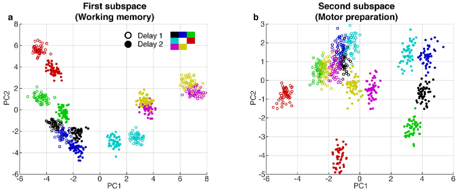
PCA projections in the first and second subspaces.
(a) Delay 1 and Delay 2 activity for 50 trials at each target location projected into the first subspace (top 2 PCs). Open circle, Delay 1 activity; closed circle, Delay 2 activity. Target locations are color coded according to the legend. Delay 2 clusters appeared to move closer to each other compared to the Delay 1 clusters. This meant that the boundaries of the classifiers trained in Delay 2 would work better for Delay 1 activity, compared to the opposite scenario, as seen in the off-diagonal quadrants in Figure 1d. (b), Delay 1 and Delay 2 activity projected into the motor preparation subspace (top 2 PCs). The clusters exhibited significant overlap during Delay 1, but separated into distinct clusters in Delay 2.
Figure 2—figure supplement 5
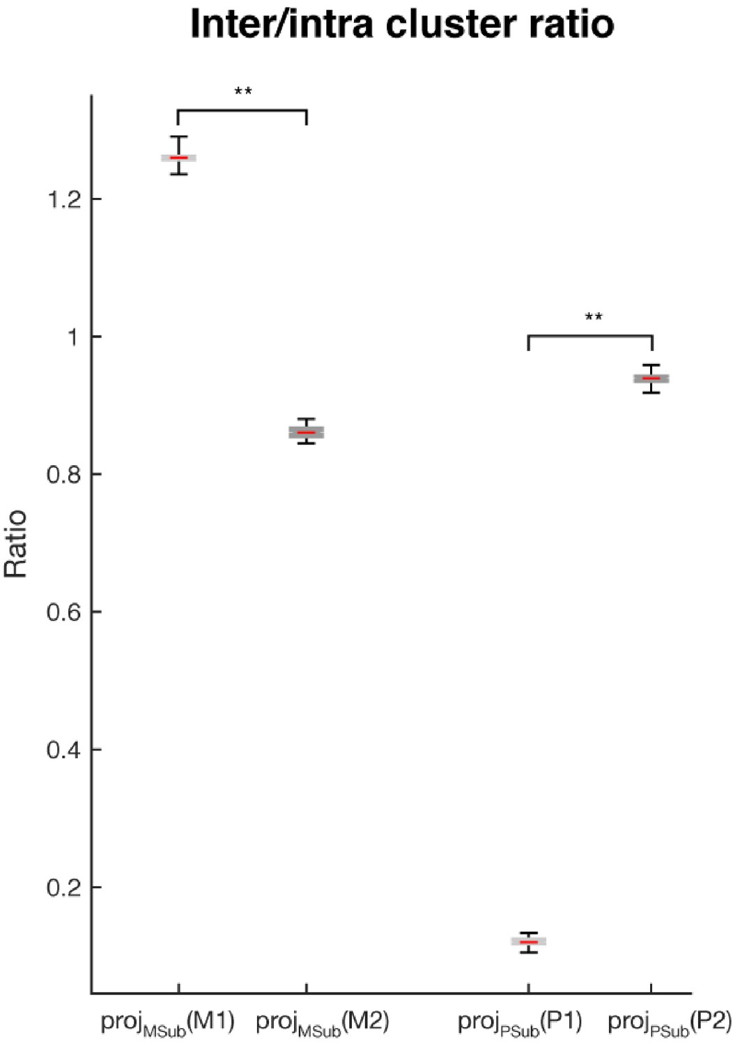
Inter- and intra-cluster distance analysis.
The ratios of the inter-cluster distance (the average of the pairwise Euclidean distance between cluster means) and the intra-cluster distance (the average of the pairwise distances between samples within each cluster, which were then further averaged across clusters) are shown for: projMSub(M1) - projection of the single-trial working memory activity in Delay 1 into the working memory subspace; projMSub(M2) – single-trial working memory activity in Delay 2 projected into the working memory subspace; projPSub(P1) – single-trial motor preparation activity in Delay 1 projected into the motor preparation subspace; and projPSub(P2) – single-trial motor preparation activity in Delay 2 projected into the motor preparation subspace. Asterisks (**), significant (i.e. 95th percentile range of the two distributions did not overlap).
Figure 2—figure supplement 6

Mean population firing rate.
We trial-averaged each cell’s firing rate according to the target condition in each time bin and then averaged across neurons. The blue line indicates the mean firing rate of the population (226 cells). The shaded area represents the standard error. The yellow line indicates time bins in which the population firing rate was significantly different from baseline (mean of the fixation period, which was 300 ms prior to the target presentation, T-test, p < 0.05).
Figure 2—figure supplement 7
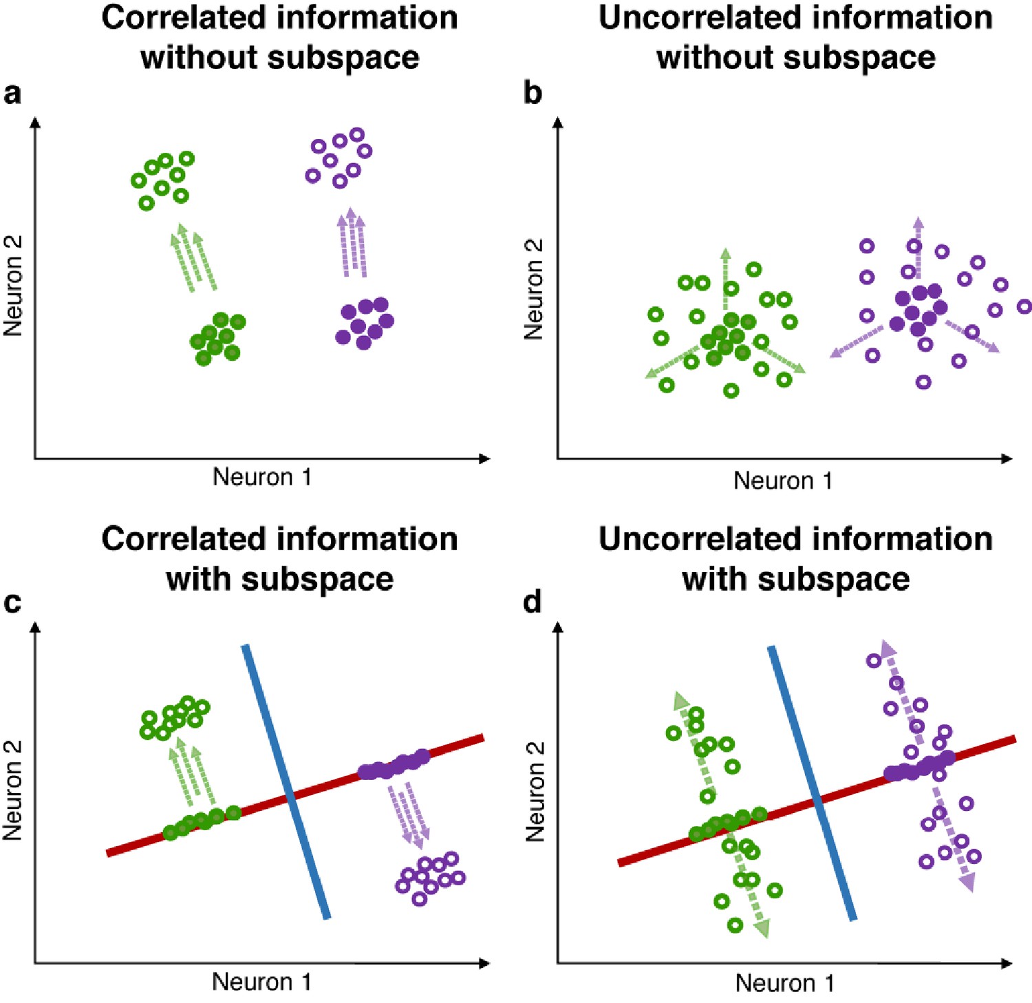
Correlated and uncorrelated information.
(a) Illustration of correlated information (in this example, two possible target locations and three possible stimulus colors, one target location is associated with only one stimulus color). Green and purple circles represent neuronal activity grouped by different target locations. Closed circles represent trial epochs containing only location information, while open circles represent trial epochs with color information incorporated into the location information. When trials are grouped by locations, the addition of correlated color activity will shift the location clusters only in the direction indicated by the parallel dashed arrows, and may not result in a decrease in the ratio of inter/intra-cluster distance. (b) In the case where target location and stimulus color are uncorrelated (each stimulus color is equally likely to appear in each target location), the addition of uncorrelated color activity (indicated by the three dashed arrows) will ‘diffuse’ clusters representing target location, thus resulting in a decrease in the ratio of inter/intra-cluster distances. (c and d) Red and blue lines represent the location and color subspaces. In both scenarios (correlated and uncorrelated information), independent location and color subspaces will alleviate the interference between the two pieces of information, as the ratio of inter/intra-cluster distance in one subspace is largely unaffected by changes in activity in the other subspace.
Figure 3 with 3 supplements

Preparatory and pre-saccadic activity.
(a) Correlation between unmixed elements found from Delay 1/Delay 2 activity (Elements 1 and 2) and the unmixed elements from Delay 1/pre saccadic activity (Elements 1’ and 2’). The matrices were flattened into 1-d for the correlation analysis. Elements 1 and 1’ were almost identical (r > 0.99, p < 0.01, left), while Elements 2 and 2’ were highly correlated (r = 0.62, p < 0.01, right). (b) Left, the percentage of cells that exhibited significant correlation between Elements 2 and 2’. Right, the percentage of cells that exhibited significant correlation between Elements 1 and 2’. The shaded area shows the 5th and 95th percentiles of the chance percentage obtained by shuffling the tuning across cells. (c) Response tuning of four representative cells that showed significant correlation between their activity in Elements 2 and 2’.
Figure 3—figure supplement 1
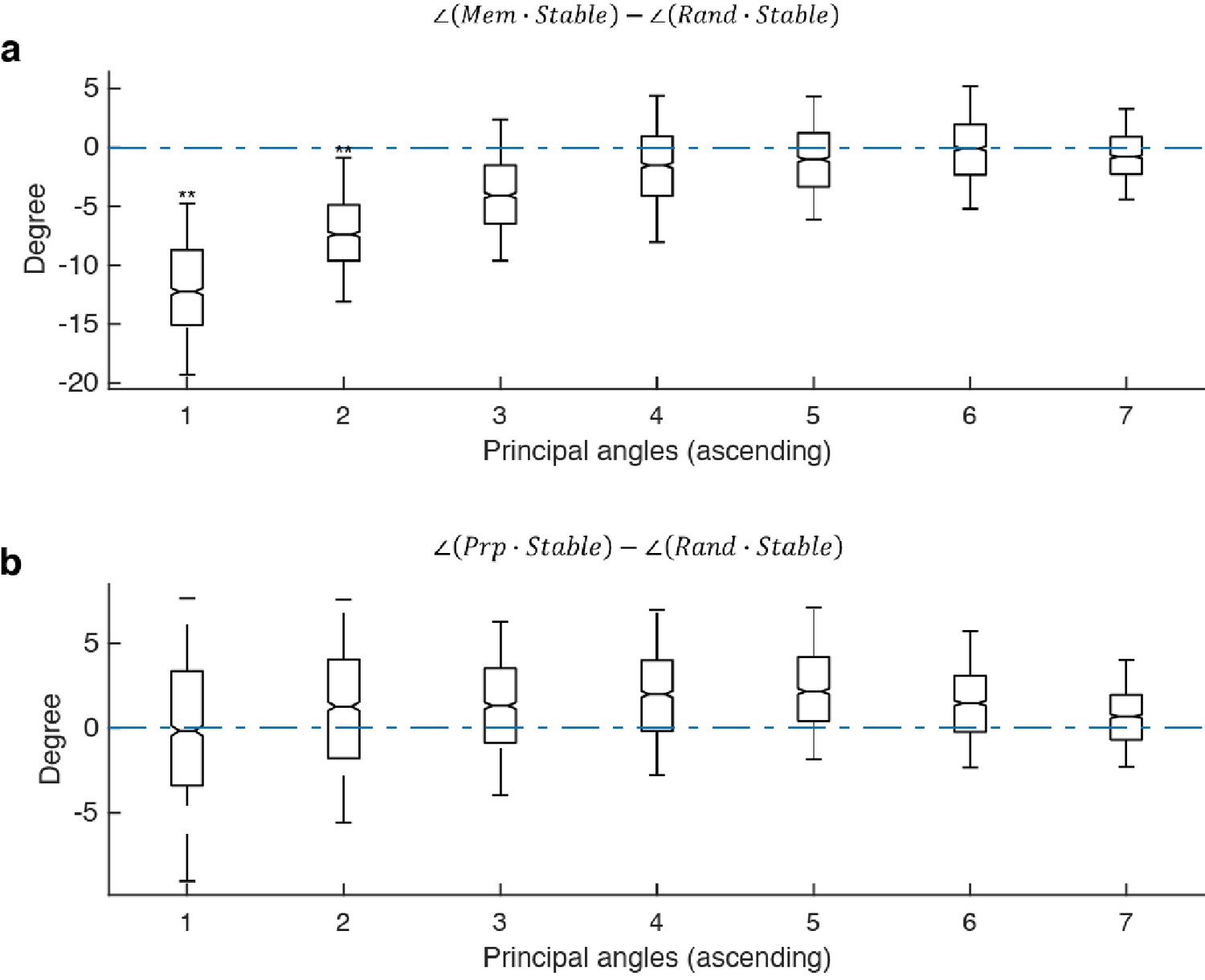
Principal angles between subspaces.
The following abbreviations are used in this figure: Mem - the working memory subspace identified in this work; Prp - the motor preparation subspace identified in this work; Stable - the stable memory subspace identified in Parthasarathy, 2019. Due to bootstrapping of pseudo-trials, different runs of the optimization gave slightly different results; and Rand - a random subspace generated from a 226 × 65 PCA space that explained 95 percent of the variance in the full-space delay activity. Each column (226 × 1) of the random subspace (226 × 7) was a random linear combination of the 65 PCs, and each column was normalized to unit length. (a), For each of the 1,000 Stable subspaces we generated, we computed the pairwise difference between its principal angles with the working memory subspace and a random subspace. The first two principal angles between the working memory subspace and the stable subspace was significantly smaller than chance, providing support that the memory subspace was similar to the stable memory subspace. (b) For each Stable subspace, we computed the pairwise difference between its principal angles with the motor preparation subspace and a random subspace. All of the principal angles between the motor preparation subspace and the stable subspace were not significantly smaller than chance, providing support that the motor preparation subspace was unrelated to the stable subspace. Asterisks (**), significant (i.e. 95th percentile range of the distribution did not overlap with zero); n.s., nonsignificant (i.e. 95th percentile range of the distribution overlapped with zero).
Figure 3—figure supplement 2
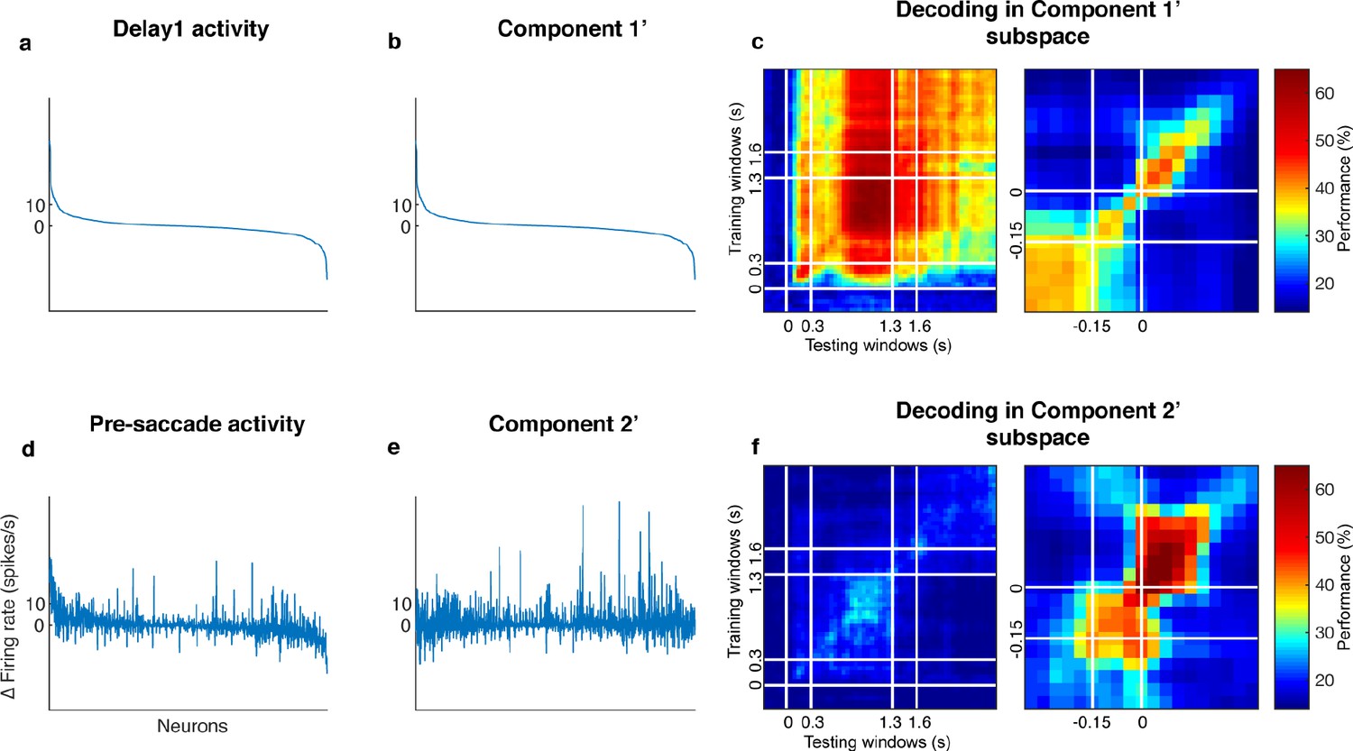
Decorrelated population activity between Delay 1 and the pre-saccadic period.
(a) Delay 1 population activity concatenated for all seven target locations. The x-axis has 1,582 points (226 cells x seven locations). Each neuron’s firing rate was time-averaged and trial-averaged for each of the seven locations, and subtracted by its baseline firing rate. The index was sorted in descending order by the Delay 1 activity in Panels a, b, d, and e. (b) The decorrelated Component 1'. (c) Cross-temporal decoding after projecting the full-space activity into the subspace defined by Component 1’. Left panel, aligned to target onset. Right panel, aligned to saccade onset. The white lines indicate the 150 ms window used to obtain the pre-saccade activity used in the decorrelation. (d) Pre-saccade period activity, significantly correlated with Delay 1 activity (r = 0.50, p < 0.01, mutual information = 0.19 bits). (e) The decorrelated Component 2’, has minimal mutual information with Component 1’ (r = −0.018, p = 0.49, mutual information = 0.087 bits). (f) Cross-temporal decoding after projecting the full-space activity into the subspace defined by Component 2’. Left panel, aligned to target onset, right panel, aligned to saccade onset.
Figure 3—figure supplement 3
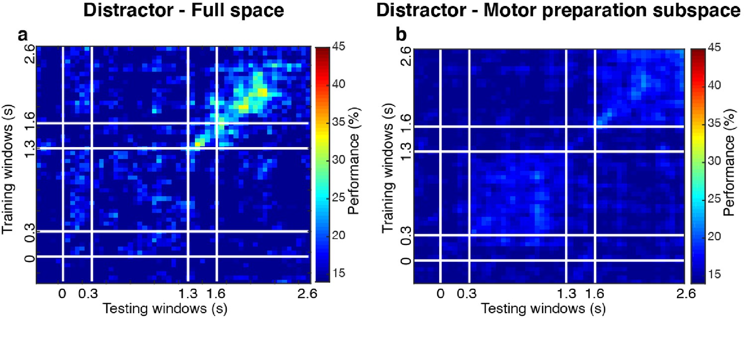
Cross-temporal decoding for distractor locations.
We grouped trials according to distractor labels (compared to grouping by target labels in the main analyses), and evaluated the decoding performance for distractor locations. (a) Distractor decoding performance in the full space (24.3 ± 1.7% in Delay 2). (b) Same as a, but after projecting data into the motor preparation subspace (17.9 ± 0.7% in Delay 2).
Figure 4 with 4 supplements
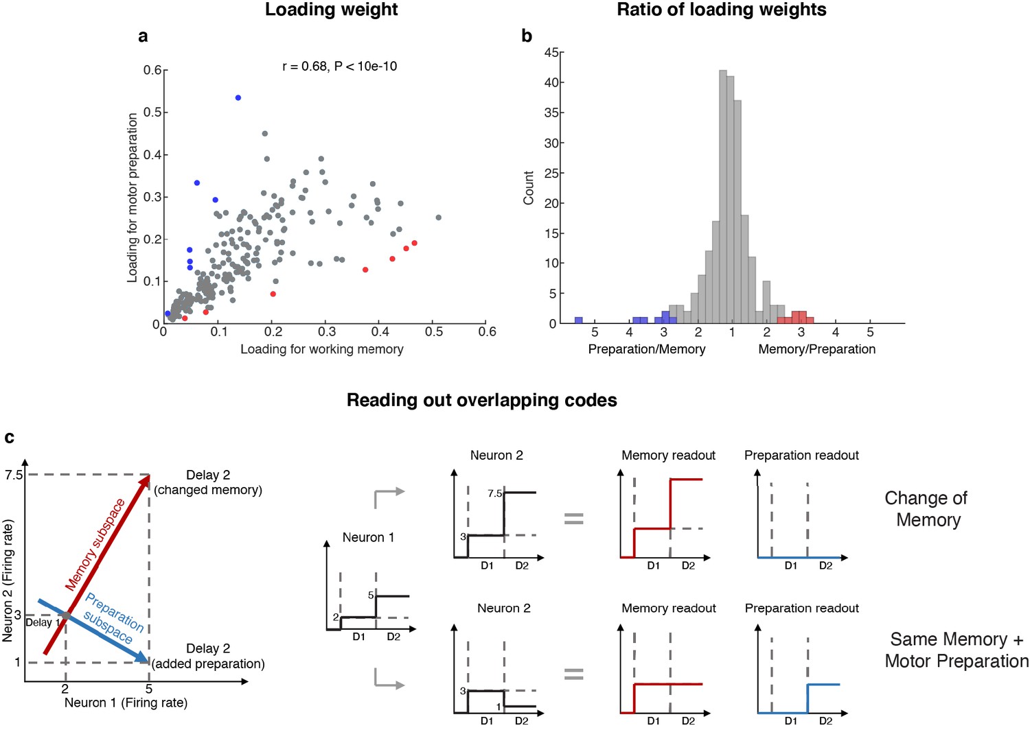
Loading weights for individual neurons.
(a) The loading weight of each neuron in the working memory subspace and the motor preparation subspace. (b) Histogram of the ratio between the loading weights for each cell. For cells with larger loading for the working memory subspace, the values are plotted to the right of the plot, while for cells with larger loading for the motor preparation subspace, the values are plotted to the left of the plot. Red dots (in a) and bars (in b) represent cells with ‘exclusive’ loading for the working memory subspace, while blue dots (in a) and bars (in b) represent cells with ‘exclusive’ loading for the motor preparation subspace. These cells were identified as those with ratios that exceeded two standard deviations from the mean. (c) Illustration of how overlapping codes can be read out. Different loading weights of the two subspaces (expressed as connection weights between the readout neurons and Neurons 1 and 2) unambiguously read out working memory or motor preparation information from the conjunctive population code formed by both Neuron 1 and Neuron 2, whereas it would have been ambiguous to look only at Neuron 1's change of firing rate in Delay 2.
Figure 4—figure supplement 1

Cross-temporal decoding on the population with mixed selectivity and populations with exclusive selectivity.
(a) Cross-temporal decoding of the 212 cells (within the two standard deviations in the ratio distribution shown in Figure 3b) in the full space. (b) Cross-temporal decoding of the 212 cells in the working memory subspace identified on the 212 cells using the same decorrelation method. (c) Cross-temporal decoding of the 212 cells in the motor preparation subspace identified on the 212 cells using the same decorrelation method. (d) Cross-temporal decoding of the seven cells with exclusive loading into the working memory subspace. (e) Cross-temporal decoding of the seven cells with exclusive loading into the motor preparation subspace.
Figure 4—figure supplement 2

Bump attractor models with and without normalization.
(a) Bump attractor model (adapted from Wimmer et al., 2014) with overlapping working memory and motor preparation populations. The full population (112 units) received two sets of inputs: 8 working memory and 8 motor preparation inputs. Each input activated sets of 10 adjacent units, and the working memory and motor preparation inputs overlapped by 43% (which matched the percentage of overlap in the LPFC data). This architecture predicts that if we sort neurons according to the working memory ‘bumps’ in Delay 1, we would be able to see the ‘bumps’ representing motor preparation in Delay 2. (b) Cross-temporal decoding of the model (without normalization) in the full space. Delay 2 decoding performance (94.1 ± 2.5%) was significantly higher than Delay 1 performance (76.9 ± 5.3%). LP11 refers to the average cross-temporal decoding performance across the bins indicated by the dashed lines where the training and testing windows were both in Delay 1, while LP22 refers to the average cross-temporal decoding performance where the training and testing windows were both in Delay 2. There was also no reduction of performance in the working memory subspace in Delay 2 (75.9 ± 7.1% in LP11, 76.6 ± 5.9% in LP22, P > 0.81, g = 0.33, figure not shown), and the mean population activity increased from Delay 1 (1.2 ± 0.04 spikes/s) to Delay 2 (1.4 ± 0.06 spikes/s, P < 0.05, g = 4.04). These three results were inconsistent with our observations from the neuronal data. (c) Schematic illustrating the increase in information without normalization. Green and purple circles represent two different target clusters in the full space separated by an inter-cluster distance of d. If correlated preparation information (in the form of inter-cluster distance of d) was added, this would result in the full-space inter-cluster distance in Delay 2 increasing by a factor of . (d) Cross-temporal decoding performance of the model (with normalization) in the full space. Delay 2 decoding performance and Delay 1 performance were not significantly different (LP22 - LP11 overlapped with 0, p > 0.69, g = 0.54). We did not observe any changes in the mean population firing rate (D1: 1.0 ± 0.04 spikes/s, D2: 1.0 ± 0.04 spikes/s, p > 0.9, g = 0.05). (e), Cross-temporal decoding performance of the model (with normalization) in the working memory subspace. Decoding performance reduced significantly in the working memory subspace in Delay 2 (84.1 ± 7.7% in LP11, 58.4 ± 4.1% in LP22, p < 0.05, g = 3.39). (f) Cross-temporal decoding performance of the model (with normalization) in the motor preparation subspace. As expected, target information in the motor preparation subspace emerged in Delay 2. (g) Single-unit activity in the attractor model. Top, a unit exclusively selective to working memory input; Middle, a unit exclusively selective to motor preparation input; Bottom, a unit showing mixed selectivity to both working memory and motor preparation inputs. (h) An example of the activity found in the model units in one trial. There was one bump in Delay 1 (blue trace), and two bumps in Delay 2 (red trace). Note that the overlapping bump in Delay 2 was smaller, which was a result of divisive normalization. (i) The memory (yellow trace) and preparation (green trace) activity unmixed from Delay 1 and Delay 2 activity. (j) The relationship between Delay 2 decoding performance (with normalization) and strength of distractor input (as a ratio compared to target input strength). Stronger distractor inputs decreased the Delay 2 decoding performance as it increased the within-cluster-variance of the data when grouped by target labels.
Figure 4—figure supplement 3
Neuronal selectivity.
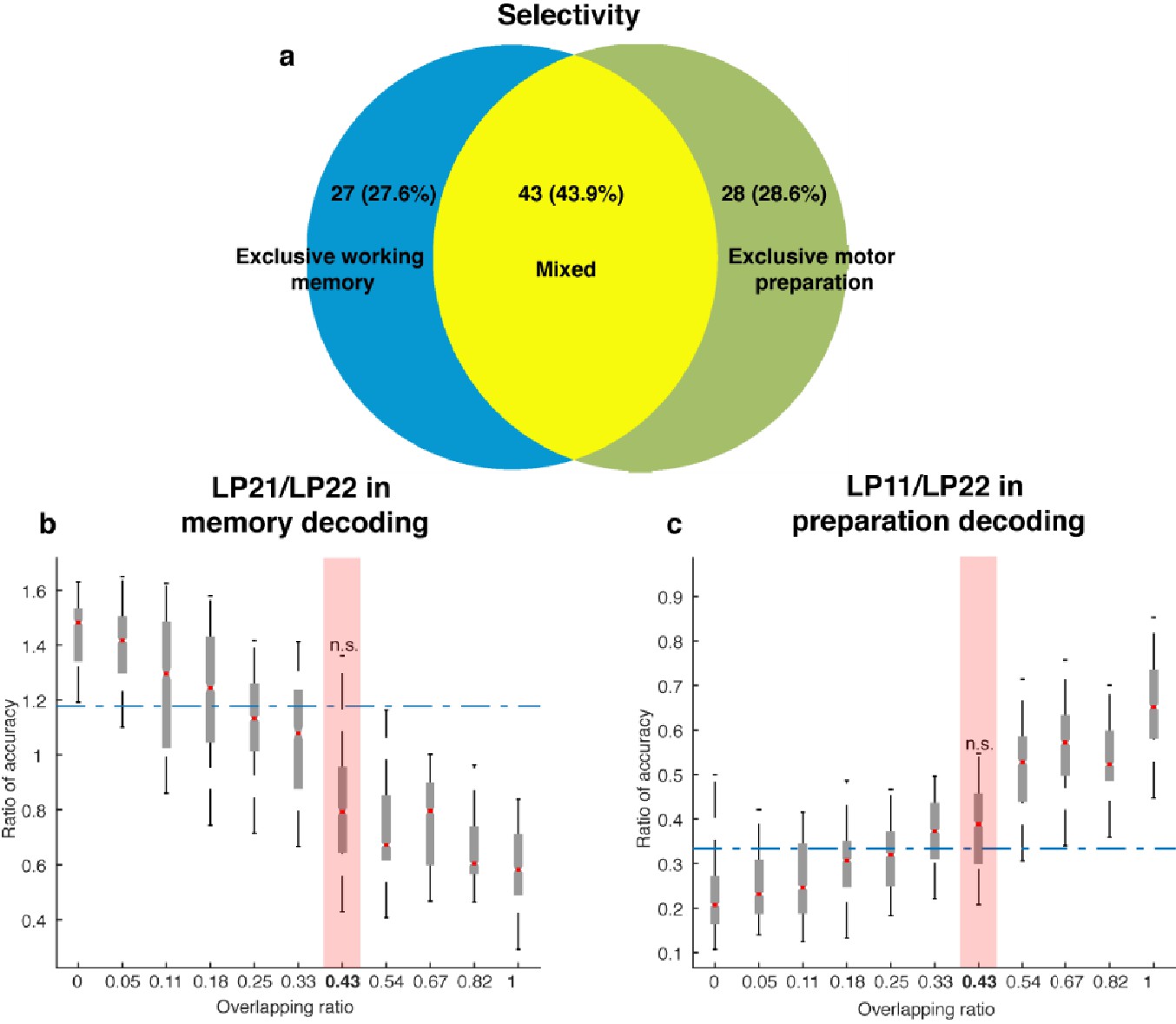
(a) In order to classify the selectivity of individual neurons, we used a two-way ANOVA with independent variables of target locations (seven locations) and task epoch (Delay 1 and Delay 2) to categorize cells as: (1) those with exclusive working memory selectivity (those with target information in both Delay 1 and Delay 2, and with selectivity to target location and task epoch, but no interaction, 27.6% of cells); and (2) those with mixed selectivity to target location and task epoch (those with a significant main effect of target location and task epoch, as well as a significant interaction between target location and task epoch, 43.9% of cells). Additionally, we used two one-way ANOVAs of target location (one in Delay 1, and one in Delay 2) to categorize cells as those with exclusive motor preparation selectivity (those with significant selectivity in Delay 2, but not Delay 1, 28.6% of cells). Among the cells that exhibited selectivity in the delay periods (98 cells), we estimated that 27.6% had exclusive working memory selectivity, 28.6% had exclusive motor preparation selectivity, and 43.9% had mixed selectivity to both working memory and motor preparation. (b) Comparison of the decoding in the working memory subspace between neural data (blue dashed line) and model data (box plots). X-axis: different population overlapping ratios between working memory and motor preparation, where overlapping ratio was the number of cells with mixed selectivity divided by the total population size. Neural data showed an overlapping ratio of 0.43. Y-axis: mean decoding accuracy in LP21 divided by mean accuracy in LP22 (refer to Figure 5e). (c) Comparison of the decoding in the preparation subspace between neural data (blue dashed line) and model data (box plots). X-axis, same as in Panel a. Y-axis, mean decoding accuracy in LP11 divided by mean accuracy in LP22 (refer to Figure 5f). n.s., nonsignificant (i.e. 95th percentile range of the distribution overlapped with the dashed line representing the result from the neural data).
Figure 4—figure supplement 4
Linear subspace model.
(a) In the linear subspace model, the stable encoding subspace was defined by the eigenvectors with eigenvalues equal to 1 (illustrated as the gray plane). Population activity outside the stable subspace would gradually decay across time and leave only the projections onto the subspace (circles on the plane). (b) Cross-temporal decoding of the model (without normalization) in the full space. Delay 2 decoding performance (86.9 ± 1.3%) was significantly higher than Delay 1 performance (65.8 ± 1.2%). This was inconsistent with our observations from the neural data. (c) Cross-temporal decoding of the model (with normalization) in the full space. Code morphing was replicated in the full space; Delay 2 decoding performance (65.0 ± 1.5%) was not significantly different from Delay 1 performance (65.0 ± 2.0%). (d) Cross-temporal decoding performance pf the model (with normalization) in the working memory subspace. The decay of working memory information was replicated in the working memory subspace identified by the unmixing method; decoding performance reduced significantly in the working memory subspace in Delay 2 (81.5 ± 1.0% in LP11, 58.8 ± 2.6% in LP22, p < 0.01, g = 11.3). (e) Cross-temporal decoding performance of the model (with normalization) in the motor preparation subspace. As expected, target information in the motor preparation subspace emerged in Delay 2. (f) The activity of three single units in the linear subspace model. All the units were mixed-selective to working memory and motor preparation inputs, because all the input loadings were distributed across the whole population (while in the bump attractor model, each input loading was restricted to only 10 adjacent units). We believe that the bump attractor model and the linear subspace model share some conceptual similarities in our case: both models have a mechanism to maintain stable activity in the absence of sustained external input, and are able to incorporate new information without affecting existing information. Further, a bump attractor model could be deemed as a special case of a linear subspace model where the reciprocally connected excitatory units are grouped together, which has more biologically support.
Figure 5 with 3 supplements
Comparisons between working memory and motor preparation subspaces.
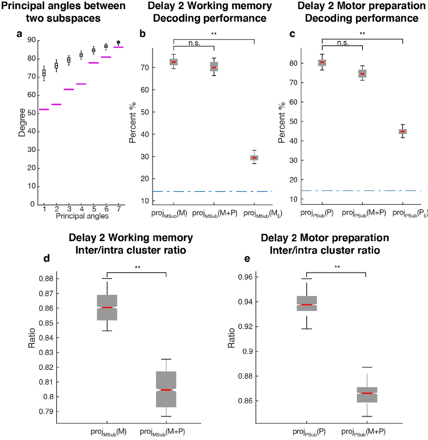
(a) The principal angles between the working memory subspace and the motor preparation subspace are shown in the magenta lines in ascending order. The black boxplots illustrate the distribution of principal angles between two random subspaces with the same dimensions as the working memory and motor preparation subspaces. The borders of the box represented the 25th and the 95th percentile of the distribution, while the whiskers represent the 5th and the 95th percentiles. (b) Decoding performance in the working memory subspace. M stands for unmixed single-trial working memory activity; projMSub(M), decoding of the unmixed single-trial working memory activity projected into the working memory subspace; projMSub(M+P), decoding of the single-trial Delay 2 activity projected into the working memory subspace; projMSub(ME), decoding of the unmixed single-trial working memory activity in error trials projected into the working memory subspace using a classifier built on unmixed single-trial working memory activity in correct trials projected into the working memory subspace; (c) Decoding performance in the motor preparation subspace. P stands for unmixed single-trial motor preparation activity. Same conventions as in a, but for unmixed single-trial motor preparation activity and the motor preparation subspace. We verified that the drop in performance in error trials was specific to the two subspaces, and not due to a non-specific increase in noise in the population (see Materials and methods). (d) Inter-to-Intra cluster ratio of unmixed single-trial working memory activity projected into the working memory subspace (projMSub(M)), and of single-trial full-space activity projected into the working memory subspace (projMSub(M+P)). (e) Same conventions as in d, but for unmixed single-trial motor preparation activity and motor preparation subspace.
Figure 5—figure supplement 1

Gram-Schmidt orthogonal decomposition.
(a) Principal angles between the working memory subspace (using the optimization method) and the first subspace from orthogonal decomposition. There were seven principal angles between two seven-dimensional subspaces. Principal angles are plotted in ascending order. The blue line shows the principle angles between the two subspaces in degrees. The black boxplots illustrate the distribution of the principal angles between the working memory subspace and 1,000 random subspaces of the same dimension. The borders of the box represented the 25th and the 95th percentile of the distribution, while the whiskers represent the 5th and the 95th percentiles. All principal angles between the working memory subspace and the first subspace obtained from the QR decomposition were significantly smaller than chance, indicating similarity between the two subspaces. (b Same as a), but between the motor preparation subspace and the second subspace from the orthogonal decomposition. Even though the orthogonal decomposition obtained similar results as our unmixed method, there are methodological limitations of using the orthogonal decomposition. First, imposing orthogonality between subspaces, while possible, may hide interesting properties in the data, since activity subspaces could be perfectly orthogonal, but they could also be non-orthogonal, such that interference between them was possible (which may account for interference between cognitive processes). As such, imposing orthogonality would prevent us from identifying interference between subspaces. Instead, the unmixing method allows for both possibilities, and hence is a more unbiased way to understand our data. Second, the unmixing method has fewer assumptions and is more flexible for subspace identification. Orthogonal decomposition imposes one fixed subspace to begin with, and the second subspace is entirely contingent to the blind choice of the first subspace. Instead, the unmixing method simultaneously identifies two subspaces without biasing toward either one.
Figure 5—figure supplement 2

| Analytical memory subspace and non-memory subspace.
(a) We calculated the difference vector between Delay 2 and Delay 1 activity (Delay 2 - Delay 1), and defined the null space of the difference vector as a stable memory subspace (which we called the Analytical memory subspace, Amem), such that the projection of Delay 1 and Delay 2 activity into this subspace overlapped. We calculated the preparation activity as the residual vector between D1, D2, and Amem, i.e. D1 - Amem, and D2 - Amem, respectively. However, this would result in a preparation activity with the same coefficients but have opposite signs in Delay 1 and Delay 2 (P1 and P2 in the figure). In other words, that implied that an ‘anti-preparation’ signal to the target location had to exist in Delay 1, and then was inverted to the ‘true preparation’ signal after distractor presentation. This seemed unnecessarily complicated, and required the existence of an ‘anti-signal’ before the ‘signal’ even emerged, which seemed unlikely for a cognitive process. (b) In order to investigate the similarity between Amem and the stable memory subspace identified in Parthasarathy, 2019, we generated 1,000 stable memory subspaces, and computed the pairwise differences between their principal angles with Amem and a random subspace (refer to Figure 3—figure supplement 1). The first three principal angles between the stable memory subspace and Amem were significantly smaller than chance, providing support that the stable memory subspace was similar to Amem. (c) Parthasarathy, 2019, we postulated a ‘non-memory’ input that was the same for all target locations that, together with a stable memory subspace, was able to capture the code morphing and the prevalence of neurons with non-linear mixed selectivity. Here, we defined the non-memory subspace as the mean of Delay 2 - Delay 1 vectors across all target locations, and performed a similar analysis as in Figure 4c in the conjunctive null space of the working memory and non-memory subspaces. Unlike the working memory and motor preparation subspaces, the working memory and non-memory subspaces were not able to capture all the target information in Delay 2 (there was significant information in the conjunctive null space), indicating that the motor preparation subspace was a better fit to the neural data than the ‘non-memory’ input.
Figure 5—figure supplement 3
| Amount of interference in different methods.
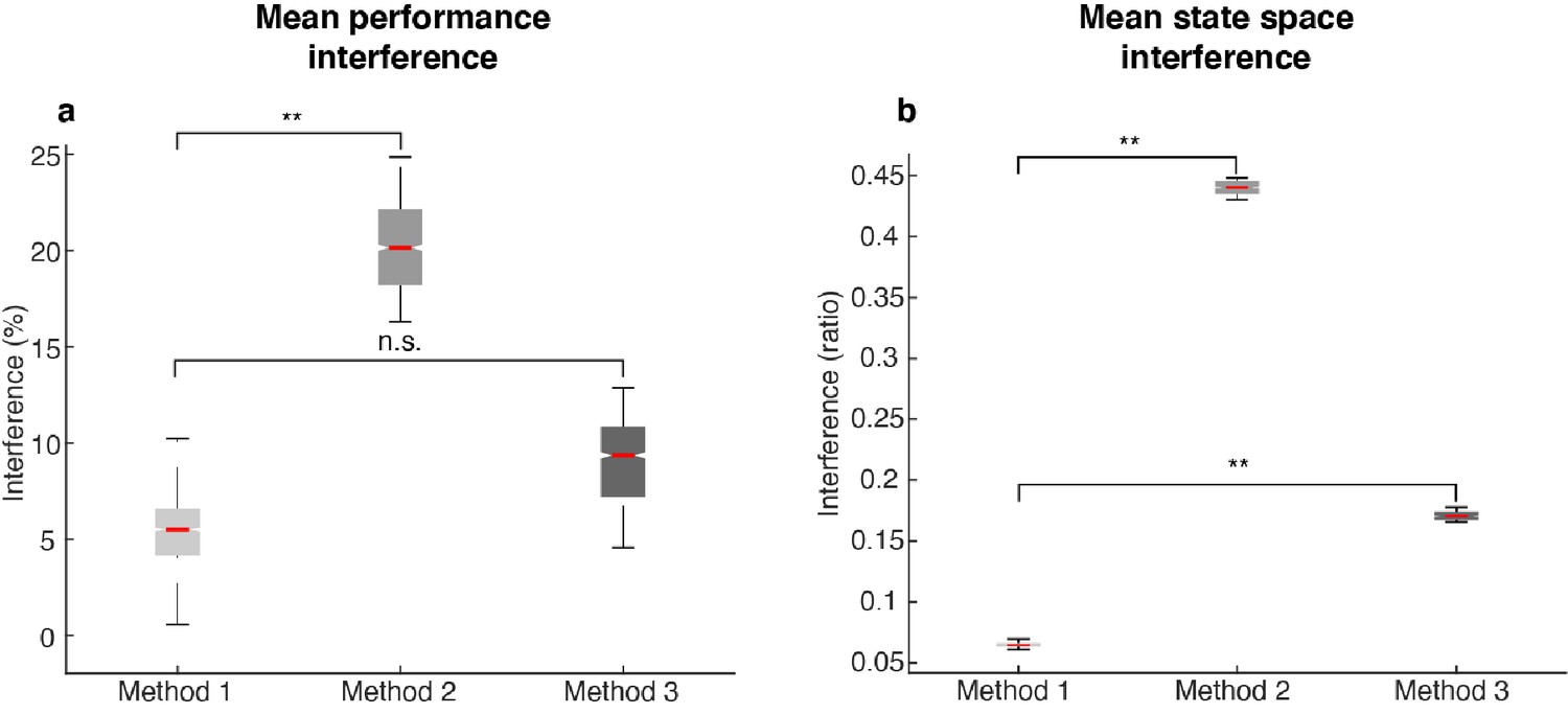
The following labels are used in this figure: Method 1 - by minimizing mutual information, we decorrelated population activity in Delay 1 and Delay 2, and found working memory and motor preparation activity with the least mutual information; Method 2 - defined Delay 1 activity as the memory activity, and the subtraction of Delay 1 from Delay 2 (D2 - D1) as the preparation activity. This method resulted in two activity arrays that were highly correlated, and thus showed a larger interference between subspaces compared to the interference found using Method 1; and Method 3 - the Analytical memory subspace defined in Figure 5—figure supplement 2. (a) Mean performance interference, as defined as in Figure 5. Method 1 showed significantly lower levels of mean performance interference than Method 2 (p < 0.001, g = 6.01), but was not significantly different from Method 3 (p > 0.67, g = 1.95). (b) Mean state space interference, defined as the inter/intra-cluster ratio for ((projMSub(M) – projMSub(M+P)) + (projPSub(P) – projPSub(M+P)))/2 in Delay 2 (refer to Figure 4d,e). Both Methods 2 and 3 showed significantly higher levels of state space interference than Method 1. Asterisks (**), significant (i.e. 95th percentile range of the two distributions did not overlap). n.s., nonsignificant (i.e. 95th percentile range of the two distributions overlapped).
Author response image 1
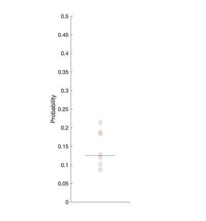
Each point represents the probability of making a saccade into the distractor location in a single session.
Blue line, chance probability (1/8). No significant evidence was found against chance (T-test, P > 0.31).
Additional files
Download links
A two-part list of links to download the article, or parts of the article, in various formats.
Downloads (link to download the article as PDF)
Open citations (links to open the citations from this article in various online reference manager services)
Cite this article (links to download the citations from this article in formats compatible with various reference manager tools)
Minimally dependent activity subspaces for working memory and motor preparation in the lateral prefrontal cortex
eLife 9:e58154.
https://doi.org/10.7554/eLife.58154


