Retinotectal circuitry of larval zebrafish is adapted to detection and pursuit of prey
- Max Planck Institute of Neurobiology, Department Genes – Circuits – Behavior, Germany
- Graduate School of Systemic Neurosciences, LMU BioCenter, Germany
Figures
Figure 1
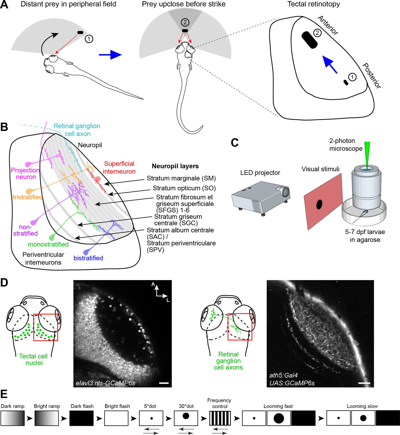
Experimental paradigm for studying location-specific processing in the tectum.
(A) In a typical hunting sequence, the fish detects prey in its peripheral visual field (1), ultimately turns and approaches to bring the prey image into its central binocular field (2). Hypothetically, the retinotectal map might be adapted to this location- and size-specific representation of the prey object. (B) Sketch of the tectum showing previously described cell types and neuropil layers. (C) Schematic for functional imaging setup. (D) On the left: Region of interest (ROI) for imaging tectal cell responses and exemplary expression of nuclear-localized GCaMP6s. On the right: ROI for RGC imaging and expression of GCaMP6s in RGC axons under control of ath5:Gal4. (E) Stimulus protocol. Arrows below stimulus representation indicate object movement, first in nasal, then in temporal direction. See Materials and methods for details. Scale bar in (D): 20 µm.
Figure 2 with 1 supplement
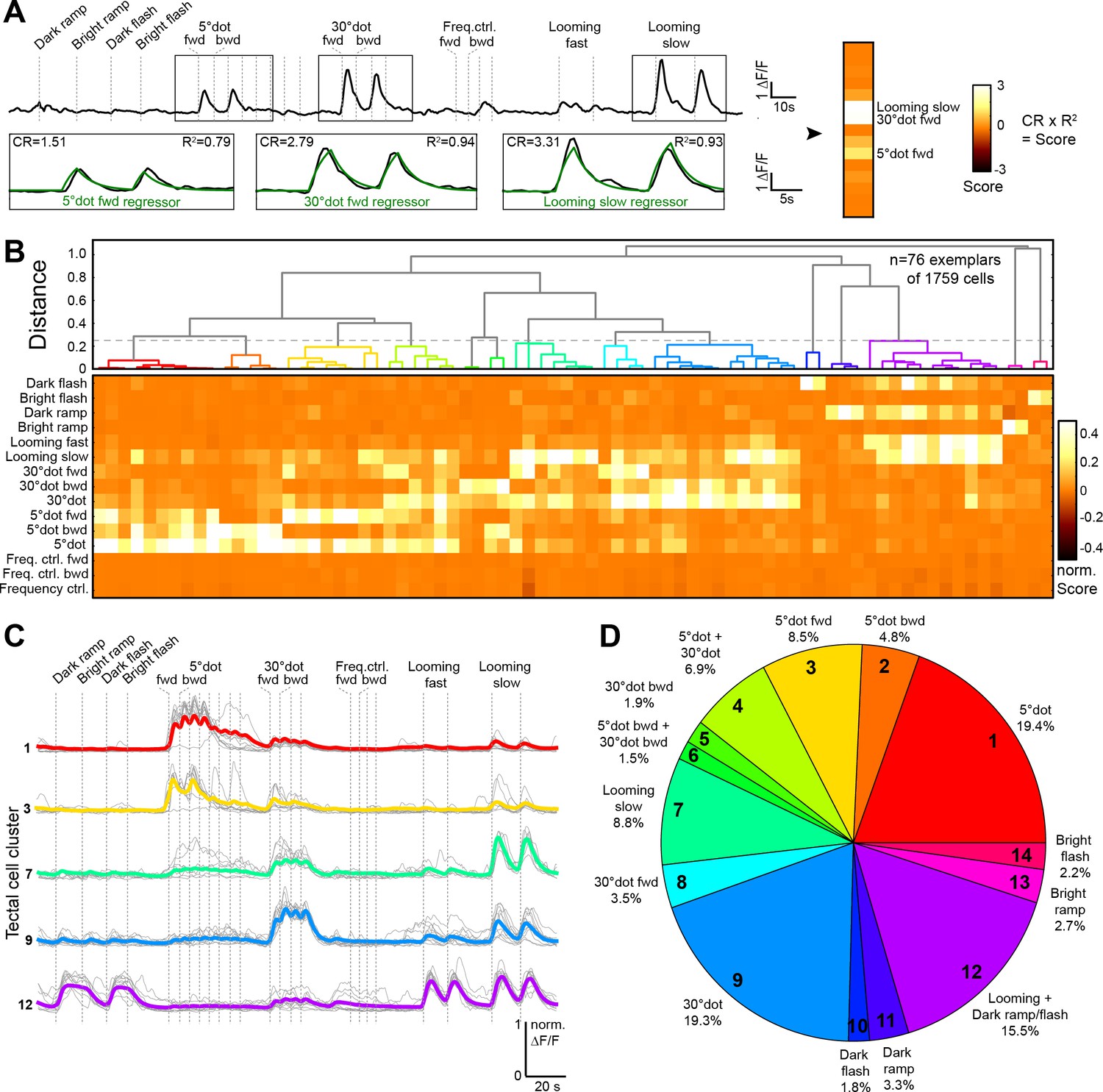
Behaviorally relevant response clusters in the tectum.
(A) Analysis of calcium imaging data. Within selected response windows (black rectangles), the ∆F/F traces were correlated to the corresponding regressor and 15 score values were calculated for each cell (CR: coefficient of regression, R2: correlation, response: black trace, model: green trace). (B) Hierarchical clustering of functional cell types in the tectum. Normalized scores for 76 exemplars, obtained by affinity propagation of 1759 cells (of three larvae) in total are shown. Dashed line indicates a chosen distance threshold of 0.25, which results in 14 functional clusters. (C) Normalized calcium transients of all exemplars (gray) and average traces of all cells (colored) for the five largest clusters. (D) Functional cluster distribution. Tectal cluster numbers are indicated.
Figure 2—figure supplement 1
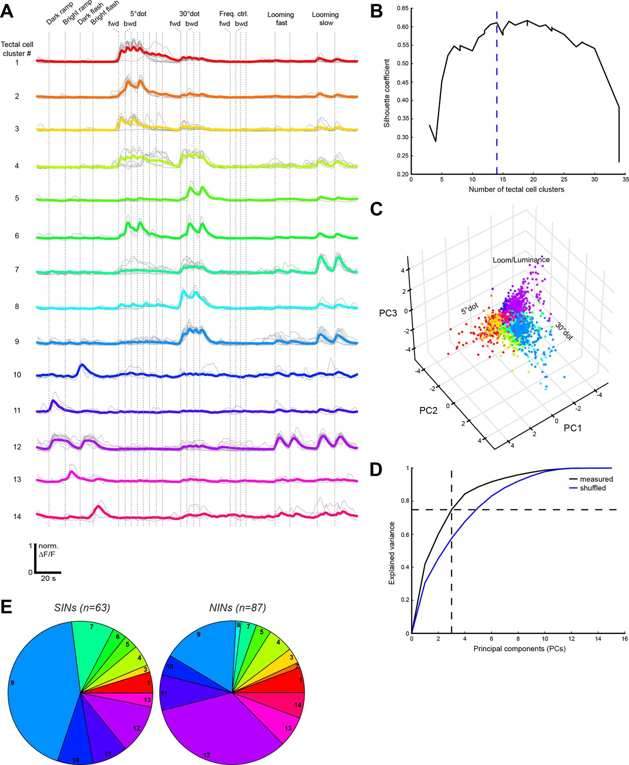
Functional clustering of tectal cells.
(A) Normalized calcium transients of all exemplars (gray) and average transients of all cells (colored) for the 14 tectal clusters. (B) Validation of cluster number by the silhouette coefficient. A minimal number of 14 clusters was chosen (dashed blue line). (C) 3D representation of the three main principal components (PCs) for all tectal cells. Data points are colored by their corresponding cluster. (D) The chosen number of three PCs explains 74.9% of the variance in the measured data (black curve). Shuffled data (blue curve) resulted in a lower average explained variance (57.6% for the three main PCs). (E) Functional cluster distribution of superficial interneurons (SINs) and neuropil interneurons (NINs), imaged in the elavl3:nls-GCaMP6s line (n = number of cells from three fish). Cluster numbers are indicated.
Figure 3 with 2 supplements
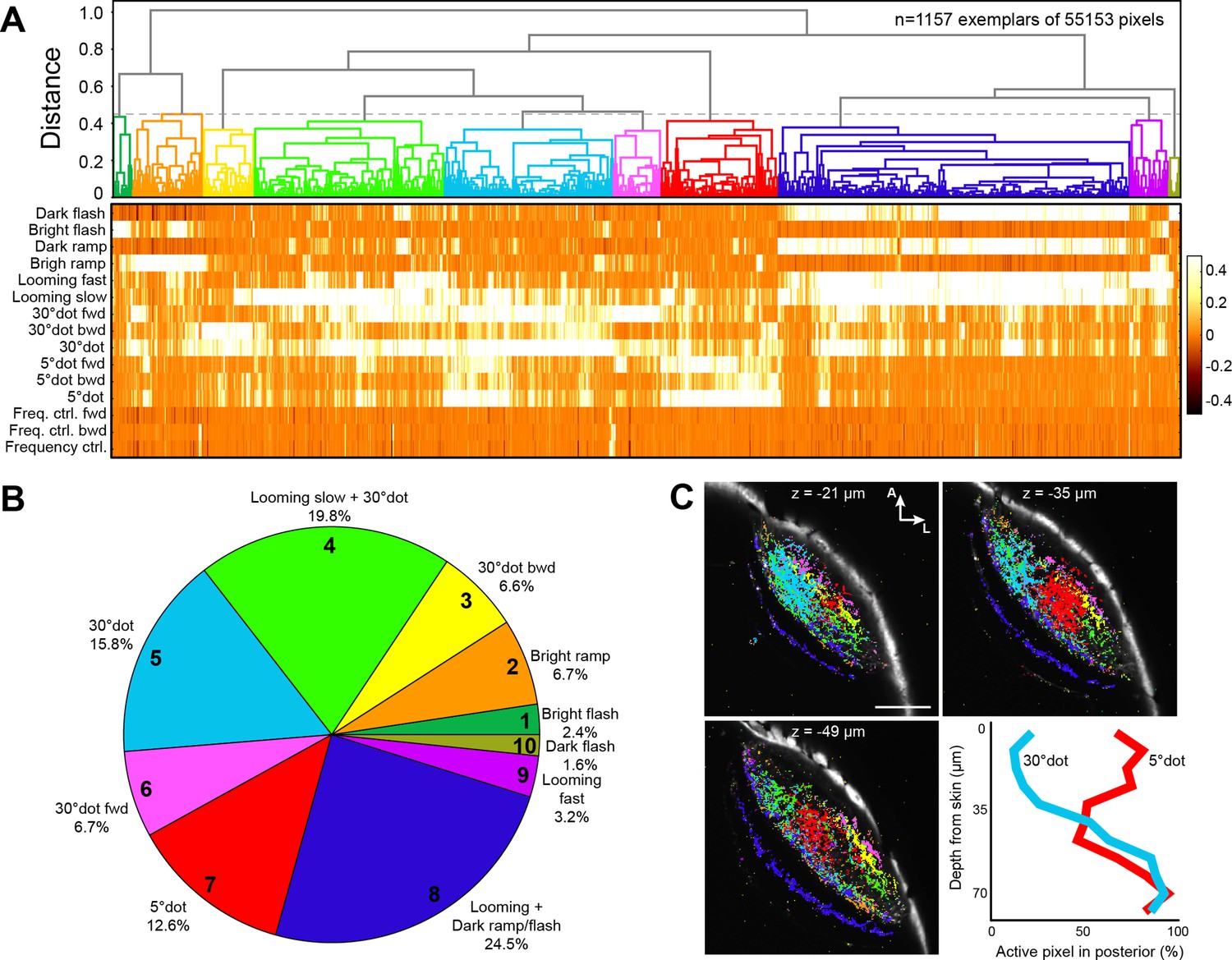
Clustering of functional RGC responses in the tectum.
(A) Hierarchical clustering of functional RGC pixels. Normalized scores for 1157 exemplars, obtained by affinity propagation of 55,153 pixels in total are shown. Dashed line indicates a chosen distance threshold of 0.45, which results in 10 functional clusters. (B) Functional cluster distribution of all analyzed RGC pixels. Cluster numbers are indicated. (C) Spatial distribution of functional RGC pixels in the tectal neuropil. Pixels were cluster-color-coded and overlaid onto single planes of the ath5:Gal4 UAS:GCaMP6s expression pattern. Z indicates plane position as the distance from dorsal skin (z = 0 µm). Last panel in (C) shows quantification of 30° dot-responsive (blue) and 5° dot-responsive (red) pixels in the posterior tectum along different z-planes. Scale bar: 50 µm.
Figure 3—figure supplement 1

Functional clustering of RGC types.
(A) Normalized calcium transients of all exemplars (gray) and average transients of all pixels (colored) for the 10 RGC clusters. (B) Silhouette plot for cluster validation. A number of 10 RGC clusters was chosen (dashed blue line) as it significantly improves the modeling correlation compared to four clusters (see Figure 4—figure supplement 1A). (C) Comparison of RGC cluster distribution for three independent larvae. Data from the first larva (first bars) are shown in Figure 2 and were used for modeling. (D) Quantification of 30° dot- (light blue), 5° dot- (red), and looming+dark ramp/flash-responsive (dark blue) pixels in the segmented tectal layers, throughout the whole image stack shown in Figure 3C.
Figure 3—figure supplement 2
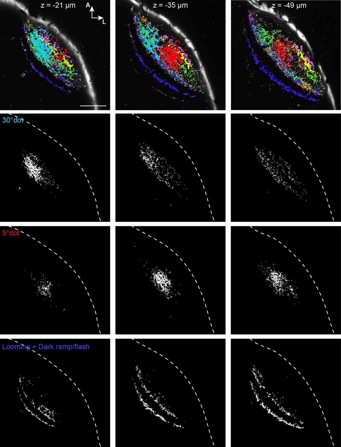
Figure panels showing the active RGC pixels of three imaging planes from Figure 3C separately for the three relevant clusters (30° dot, 5° dot, looming+dark ramp/flash).
Skin is outlined by white-dashed line. Scale bar: 50 µm.
Figure 4 with 1 supplement
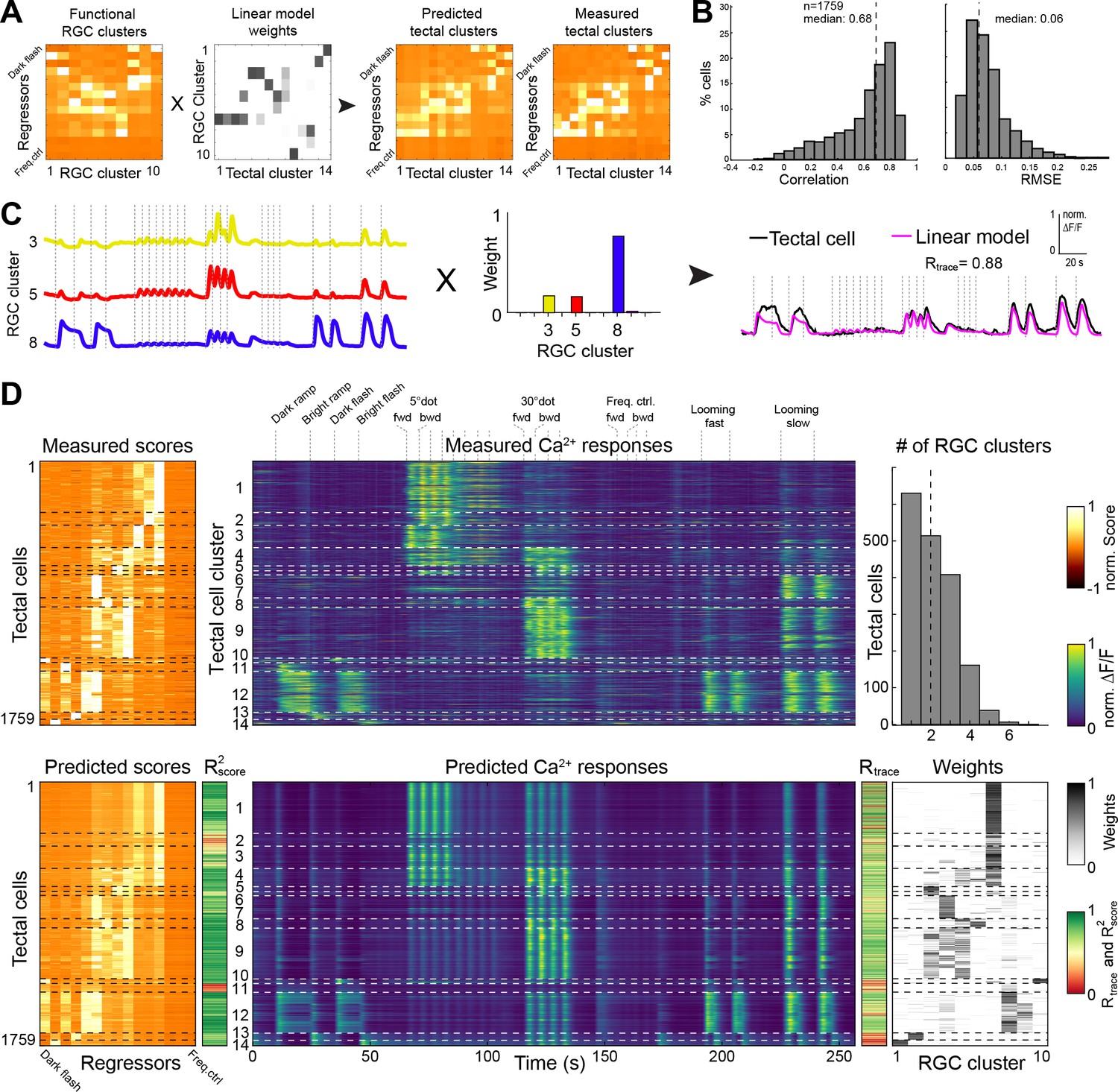
Modeling of tectal responses by linear combinations of RGC inputs.
(A) Modeling workflow. Tectal cluster scores were predicted by a linear combination of weighted RGC cluster scores and finally compared to previously measured tectal scores. For color scale, see (D). (B) Prediction quality for modeling the scores of each sampled tectal cell (n = 1759). Left graph shows the correlation between predicted and measured scores. Right graph shows distribution of root mean squared errors of the cross-validated model (see Materials and methods for details). (C) Example for modeling the calcium response of a single tectal cell from weighted average responses of three RGC clusters. (D) Summary of modeling scores (left), calcium responses (middle), and weights (lower right) for all tectal cells (n = 1759). Functional tectal clusters are indicated by dashed horizontal lines. Color scales are shown on the right. Upper graph on the right shows the distribution of the number of RGC clusters used for modeling tectal responses. Dashed vertical line indicates a median of two RGC clusters.
Figure 4—figure supplement 1

Linear modeling parameters.
(A) Modeling prediction quality shown as correlation values R2score and Rtrace, as a function of RGC cluster number. (B) Mean squared error (MSE) of modeling prediction as a function of the regularization parameter λ. See Materials and methods for details. (C) Correlation (R) between predicted and measured scores for modeling data (green) compared to a randomized model (gray). See Materials and methods for details.
Figure 5 with 3 supplements

Dendrite morphologies of functionally identified tectal neurons match input layers.
(A) The FuGIMA-f construct, which allows coexpression of nuclear-localized GCaMP6f and photoactivatable GFP (paGFP), was combined with Gal4s1101t for panneuronal expression and elavl3:lyn-tagRFP for image registrations. (B) Workflow of single-cell photoactivation, cell tracing, landmark registrations and layer quantifications (see Materials and methods for details). (C) Morphological barcode for the cell in (B). (D) Sideview of registered FuGIMA cells in the tectum of a standard brain. Tectal neuropil is shaded in gray. (E) Average proportional branch length of neurites in the respective tectal layers, quantified for 30° dot- (blue), 5° dot- (red), and looming- (purple) responsive cells. Statistically significant differences between 5° dot- and looming-responsive cells are indicated by stars. For comparison, the quantification of RGC input in the respective layers is shown in the back (see Figure 3—figure supplement 1D). Error bars are SEM. ***: p < 0.001, **: p < 0.01, and *: p < 0.05. (F) Exemplary tectal cell morphotypes identified for the response groups described above. PVIN: periventricular interneuron; ns: non-stratified; bs: bistratified; ts: tristratified. Scale bar in (B): 20 µm.
Figure 5—figure supplement 1
Comparison and quantification of tectal cell morphologies.
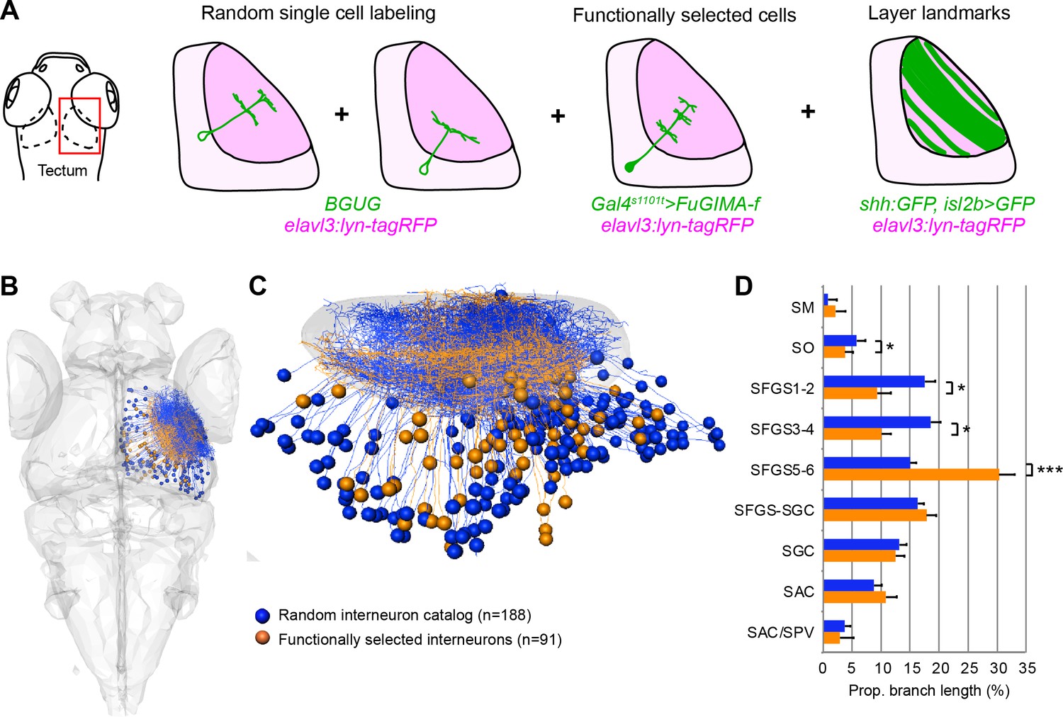
(A) Workflow for combining single-cell data. A common reference marker (elavl3:lyn-tagRFP) allowed co-registration of randomly labeled single cells (BGUG method), functionally selected single cells (FuGIMA method), and RGC expression patterns as landmarks for tectal laminae. (B) Dorsal overview of collected tectal interneurons from BGUG dataset (blue) and FuGIMA dataset (orange). (C) Tectal sideview. Dorsal is up and anterior is left. (D) Average proportional branch length of tectal cell neurites in the respective layers, for randomly labeled (blue) and functionally selected cells (orange). Error bars are SEM. ***: p < 0.001, and *: p < 0.05.
Figure 5—figure supplement 2
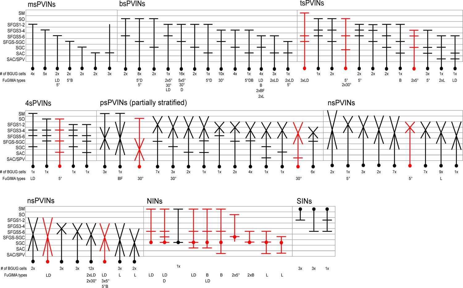
Tectal interneuron catalog.
Schematic representation of all identified morphotypes for tectal interneurons. The number of collected BGUG cells for each type is presented below. Red morphotypes have only been identified by the FuGIMA method. Identified functional types are indicated below. L: looming, D: dark ramp, B: bright ramp, 5°: small dot, 30°: big dot, BF: bright flash. PVIN: periventricular interneuron, NIN: neuropil interneuron, SIN: superficial interneuron, ms: monostratified, bs: bistratified, ts: tristratified, 4 s: tetrastratified, ps: partially stratified, ns: non-stratified/diffuse.
Figure 5—figure supplement 3
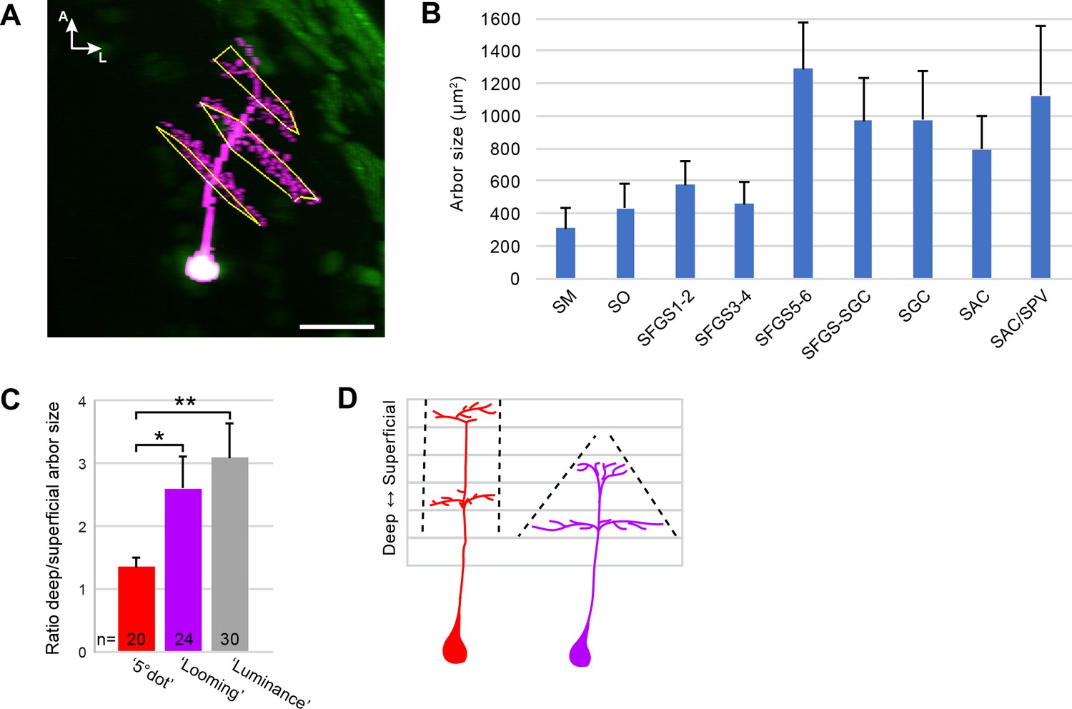
Quantification of tectal cell arbor size.
(A) Illustration of arbor quantification for a tristratified tectal cell. (B) Average arbor area in different tectal laminae. Error bars are SEM. (C) Ratio of deep vs. superficial arbor area within the same cells, for 5° dot-, Looming-, and Luminance-responsive cell types. Error bars are SEM. **: p < 0.01, and *: p < 0.05. (D) Illustration of columnar-shaped, 5° dot-responsive cells (red) and cone-shaped, looming-responsive cells (purple).
Figure 6
Functional compartmentalization of the tectum along the anterior-posterior axis.
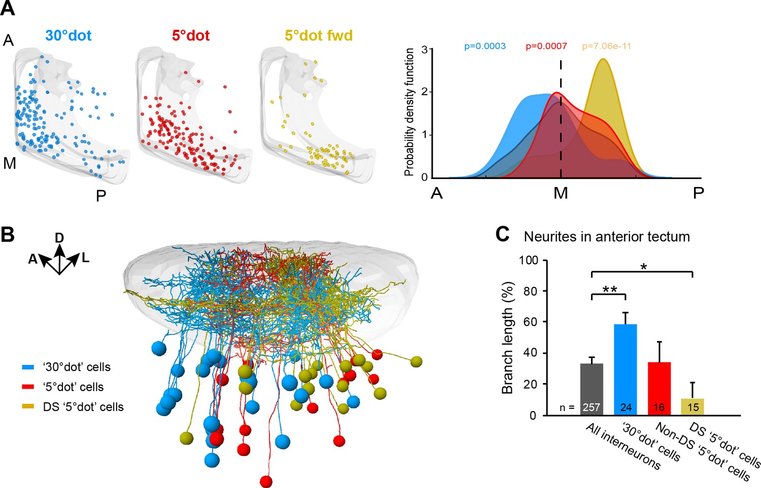
(A) Distribution of tectal cell bodies from 30°-dot (blue), 5°-dot (red) and 5°-dot-forward (yellow) response clusters. Anterior (A), medial (M) and posterior (P) positions of the tectum are indicated. Graph shows probability density function for cell body distribution. Integrals are colored according to their functional cluster with p-values characterizing the difference from the distribution of all sampled cells (gray integral). (B) Tectal sideview of registered FuGIMA neurons showing the distribution of 30°-dot (blue), 5°-dot non-DS (red) and 5°-dot-DS (yellow) cells. (C) Quantification of proportional neurite branch length of tectal cells in the anterior tectum. N equals number of cells. **: p = 0.006,; *:p = 0.014.
Figure 7

Small size-tuned RGC inputs are essential for small-object processing in the tectum.
(A) Experimental setup for RGC axon ablations. Larvae are expressing mCherry in RGCs and nulear GCaMP6s panneuronally. The eye contralateral to the ablation site is visually stimulated and the ipsilateral tectal cells are functionally imaged before and after the ablations. As a control, the eye ipsilateral to the ablation site is stimulated and the contralateral tectal cells are imaged in the same fish. (B) Sideview of mCherry expression in RGCs at 6 dpf shows the most lateral axon bundle, which leaves AF7 for the SO layer (arrow). (C) Dorsal view of single image planes showing the axon fibers of interest in the contralateral (control, upper panel) and ipsilateral (ablated, lower panel) pretectum of the same fish. (D) Single functional image planes, projected over time, showing nuclear GCaMP6s expression in the ipsilateral tectum, before (6 dpf, left) and after (7 dpf, right) ablation. Pixels are color-coded by preference for 5° dot (magenta) or looming (cyan) stimuli. (E) Number of cells per image plane (out of two fish), which are responsive to a 5° dot stimulus, before and after ablations in the ipsilateral and the contralateral tectum. (F) Same as (E), showing the number of cells responsive to a looming stimulus. (G) Fraction of 5°-dot- and looming-responsive cells after ablations in the ipsilateral and contralateral tectum. Error bars are SEM. ***: p = 0.0006; n.s.: p = 0.46. N equals number of cells from two independent fish. Scale bars in (B): 30 µm, (C): 20 µm, and (D): 50 µm.
Figure 8 with 1 supplement

Large-object processing cells are required for hunting behavior.
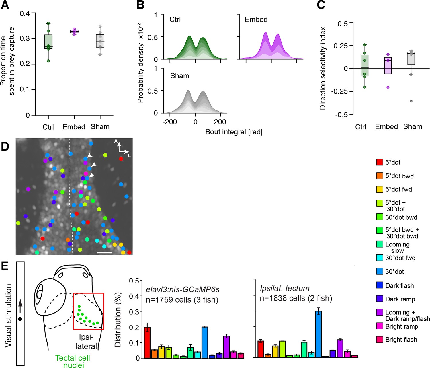
(A) 7 dpf old fish panneuronally expressing nuclear-localized GCaMP6s (green) were visually stimulated and imaged. Tectal cells were functionally identified (cluster-colored circles) and selected for ablations (arrowheads). At dpf, hunting behavior was analyzed in free-swimming larvae. (B) Proportion of time larvae spent engaged in hunting behavior, having their eyes converged. Single data points represent individual fish. 'Sham' (gray): control larvae with ablations of non-responsive cells, '5°' (red): unilateral ablations of 5°-dot-responsive cells in the right tectum, '30°' (blue): unilateral ablations of 30°-dot-responsive cells in the right tectum, 'bi-30°': bilateral ablations of 30°-dot-responsive cells. *: p = 0.02, **: p = 0.006, n.s.: p = 0.15. (C) Probability density plots of bout integrals for the initial J-turns, with positive values indicating a rightward and negative values indicating a leftward turn. Color shading indicates accumulated data for individual fish. (D) Direction selectivity index for initial J-turns of individual fish. *: p = 0.029, n.s.: p > 0.05. (E) Ethological relevance for A-P distribution of functionally distinct tectal cells. Before initiation of prey capture behavior, small moving objects are likely spotted in the temporal, monocular visual field. Precise recognition and processing of object movement by posterior DS cells avoids losing the object and enables adapted orientation turns towards the object. During prey pursuit, prey size seemingly increases and is detected by large-dot-responsive cells in the anterior tectum. Eye convergence allows binocular processing of object size and movement.
Figure 8—figure supplement 1
Tectal cell ablation controls and enucleation experiments.
(A–C) In our free-swimming prey capture assay, 'sham' ablated larvae (gray), in which non-responsive tectal cells have been removed, did not behave differently from untreated ('ctrl', green), or agarose-embedded and released ('embed', purple) larvae, in terms of time spent in prey capture (A), initial J-turn kinematics (B), or direction selectivity index (C). (D) Cluster color-coded functional cell responses in both anterior tecta for the experiment shown in Figure 8A (arrow heads highlighting cells selected for ablations). Midline is indicated by a dashed white line. Note the tectal cell responses in the left, non-stimulated tectum. (E) Enucleated larvae expressing elavl3:nls-GCaMP6s were functionally imaged as described, and the functional cluster distribution of tectal cells was compared to untreated fish. Error bars are SEM. Functional cluster colors are described on the right. Scale bar in (D): 20 µm.
Tables
Key resources table
| Reagent type (species) or resource | Designation | Source or reference | Identifiers | Additional information |
|---|---|---|---|---|
| Chemical compound, drug | Alpha-Bungarotoxin | Invitrogen | Invitrogen:B1601 | |
| Chemical compound, drug | Tricaine | Sigma-Aldrich | Sigma-Aldrich:MS-222 | |
| Genetic reagent (Danio rerio) | Tg(elavl3:nls-GCaMP6s)mpn400 | Förster et al., 2017 | ZFIN ID: ZDB-ALT-170731-37 | |
| Genetic reagent (Danio rerio) | Tg(atoh7:Gal4-VP16)s1992t (ath5:Gal4) | Del Bene et al., 2010 | ZFIN ID: ZDB-FISH-150901-27082 | |
| Genetic reagent (Danio rerio) | Tg(UAS:GCaMP6s)mpn101 | Thiele et al., 2014 | ZFIN ID: ZDB-FISH-150901-22562 | |
| Genetic reagent (Danio rerio) | Et(E1b:Gal4-VP16)s1101t | Scott et al., 2007 | ZFIN ID: ZDB-FISH-150901-5255 | |
| Genetic reagent (Danio rerio) | Tg(elavl3:lyn-tagRFP)mpn404 | Dal Maschio et al., 2017 | ZFIN ID: ZDB-ALT-170731-38 | |
| Genetic reagent (Danio rerio) | Tg(isl2b:Gal4-VP16, myl7:TagRFP)zc65 | Fujimoto et al., 2011 | ZFIN ID: ZDB-FISH-150901-13523 | |
| Genetic reagent (Danio rerio) | Tg(14xUAS:EGFP)mpn100 | Thiele et al., 2014 | ZFIN ID: ZDB-GENO-140812-1 | |
| Genetic reagent (Danio rerio) | Tg(Shha:GFP)t10 | Neumann and Nuesslein-Volhard, 2000 | ZFIN ID: ZDB-GENO-060207-1 | |
| Genetic reagent (Danio rerio) | Tg(UAS:mCherry)s1984t | Heap et al., 2013 | ZFIN ID: ZDB-FISH-150901-14417 | |
| Genetic reagent (Danio rerio) | Tg(brn3c:GAL4, UAS:gap43-GFP)s318t (BGUG) | Xiao and Baier, 2007 | ZFIN ID: ZDB-ALT-070423-6 | |
| Genetic reagent (Danio rerio) | Tg(UAS:paGFP,nlsGCaMP6f)mpn104 (UAS:FuGIMA-f) | This paper | Tol2-mediated transgenesis | |
| Software, algorithm | Imaris | Bitplane | http://www.bitplane.com | |
| Software, algorithm | ImageJ/Fiji | Schindelin et al., 2012 | http://fiji.sc | |
| Software, algorithm | MorphoLibJ (ImageJ plugin) | Legland et al., 2016 | http://imagej.net/morpholibj | |
| Software, algorithm | PsychoPy2 | Peirce, 2007 | http://www.psychopy.org | |
| Software, algorithm | Python 2.7 | Python.org | http://www.python.org | |
| Software, algorithm | Python 3 | Python.org | http://www.python.org | |
| Software, algorithm | CaImAn (Calcium Imaging Analysis toolbox) | Giovannucci et al., 2017 | http://github.com/flatironinstitute/CaImAn | |
| Software, algorithm | NeuTube | Feng et al., 2015 | http://www.neutracing.com | |
| Software, algorithm | Advanced Normalization Tools (ANTs) | Avants et al., 2010 | http://stnava.github.io/ANTs | |
| Software, algorithm | RStudio Version 1.0.136 | RStudio | http://www.rstudio.com | |
| Software, algorithm | R package nat (NeuroAnatomy Toolbox) | Bates et al., 2020 | http://jefferis.github.io/nat/ | |
| Software, algorithm | 3DSlicer | Fedorov et al., 2012 | http://www.slicer.org | |
| Software, algorithm | Plotly Chart Studio | Plotly.com | http://www.plotly.com | |
| Software, algorithm | Custom tracking and behavior analysis code | Mearns et al., 2020 | http://bitbucket.org/mpinbaierlab/mearns_et_al_2019 |
Additional files
Download links
A two-part list of links to download the article, or parts of the article, in various formats.
Downloads (link to download the article as PDF)
Open citations (links to open the citations from this article in various online reference manager services)
Cite this article (links to download the citations from this article in formats compatible with various reference manager tools)
Retinotectal circuitry of larval zebrafish is adapted to detection and pursuit of prey
eLife 9:e58596.
https://doi.org/10.7554/eLife.58596


