Figures and data in The biomechanical role of extra-axonemal structures in shaping the flagellar beat of Euglena gracilis | eLife

Figures
Videos
Additional files

11 figures, 3 videos and 2 additional files

Figures

Figure 1

Download asset Open asset

Inner structure of Euglena gracilis' flagellum.

(a) A specimen of freely swimming Euglena gracilis, and (b) a sketch of the cross-section of its flagellum, as seen from the distal end. The flagellar inner structure is composed by the paraflagellar rod (PFR, textured), and the axoneme (Ax). The PFR is connected via bonding links to the axonemal doublets 1, 2, and 3. The inner structure of the flagellum is enclosed by the flagellar membrane (dotted contour). By inhibiting MTs’ sliding, the PFR selects the spontaneous bending plane of the Ax (dashed line). As a key geometric feature, the solid line that joins the Ax center $𝐫^{a}$ and the PFR center $𝐫^{p}$ crosses at an angle $ϕ^{p}$ the spontaneous bending plane. Doublets are numbered following the convention adopted in the electron microscopy studies Melkonian et al., 1982 and Bouck et al., 1990, to facilitate comparison. The opposite convention, in which microtubules are numbered in increasing order in the anti-clockwise direction when seen from the distal end of the Ax, is far more common in structural studies of cilia.

Figure 2

Download asset Open asset

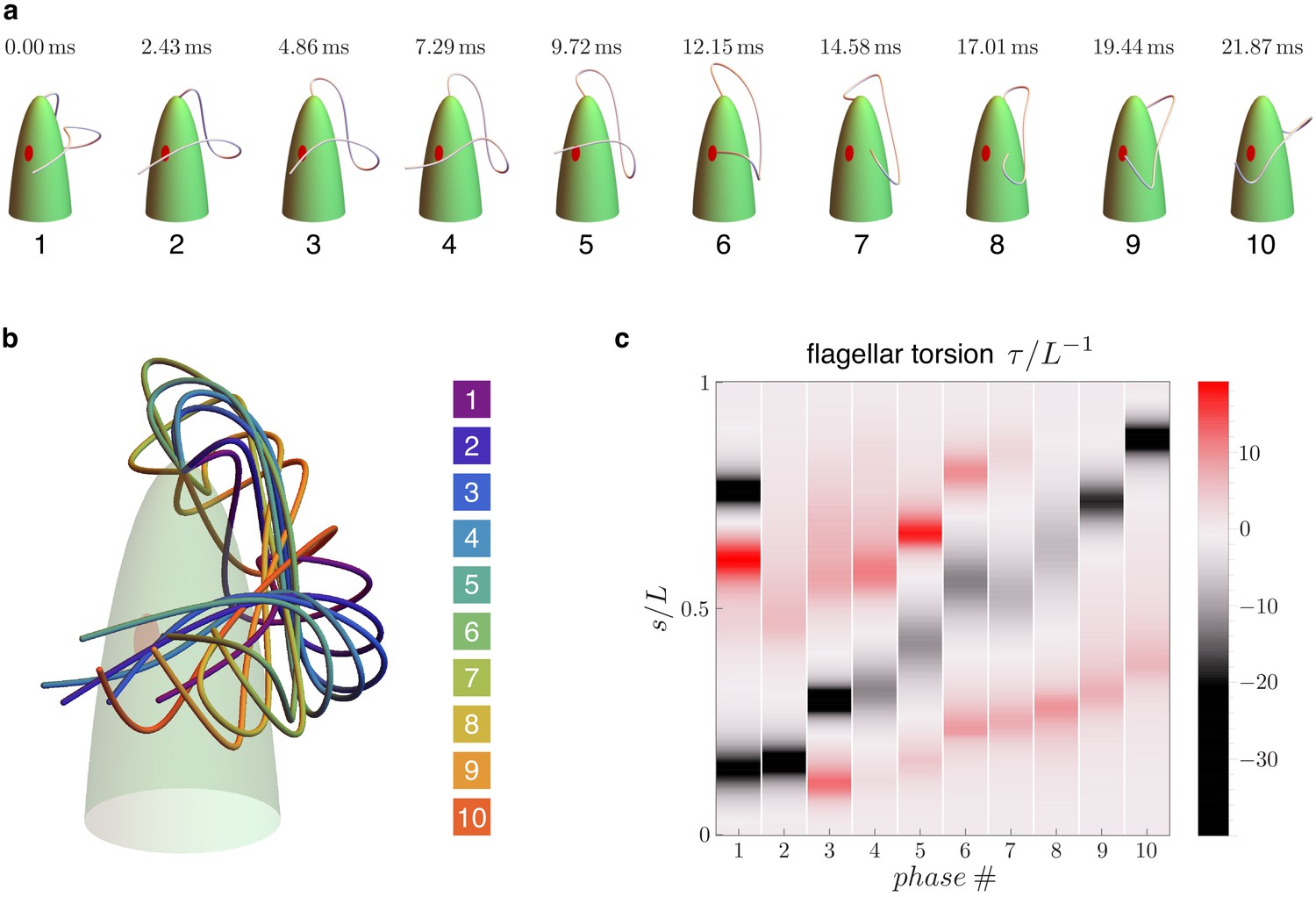
Flagellar beat kinematics of freely swimming Euglena gracilis.

(a) $N = 10$ flagellar configurations in evenly spaced instants (phases) within a periodic beat. (b) The same configurations overlapped and color coded according to their phases. (c) Computed torsion $τ = τ (s)$ as a function of the flagellar arc length $s$ . The plot is presented in terms of the normalized quantities $τ / L^{- 1}$ and $s / L$ , where $L$ is the total length of the flagellum. Panels (a-b) are adapted from Figure 5.E of Rossi et al., 2017.

Figure 2—source code 1 Experimental flagellar waveforms and torsion calculator.: https://cdn.elifesciences.org/articles/58610/elife-58610-fig2-code1-v2.zip
Download elife-58610-fig2-code1-v2.zip

Figure 3

Download asset Open asset

Flagellar beat of capillary trapped specimens.

(a) A specimen of Euglena gracilis trapped at the tip of a capillary (bottom). The typical outline of its beating flagellum is that of a looping curve, which is consistent with the outline of a simple curve with two concentrated torsional peaks of alternate sign along the length of the curve, that is, a torsion dipole (top). (b) Close-up images of the same specimen of capillary-trapped (CT) E. gracilis as seen from different viewpoints, upon successive ∼90° turns of the capillary tube. The body orientation with respect to the objective is estimated from the anatomy of the cell, and in particular from the position of the eyespot (a visible light-sensing organelle present on the cell surface). Microscopy images are decorated with the tracked outlines of the flagellum in different phases (same color coding as in Figure 2). The outlines (2d projections) of the 3d reconstructed flagellar beat of freely swimming (FS) specimens are shown for comparison.

Figure 4

Download asset Open asset

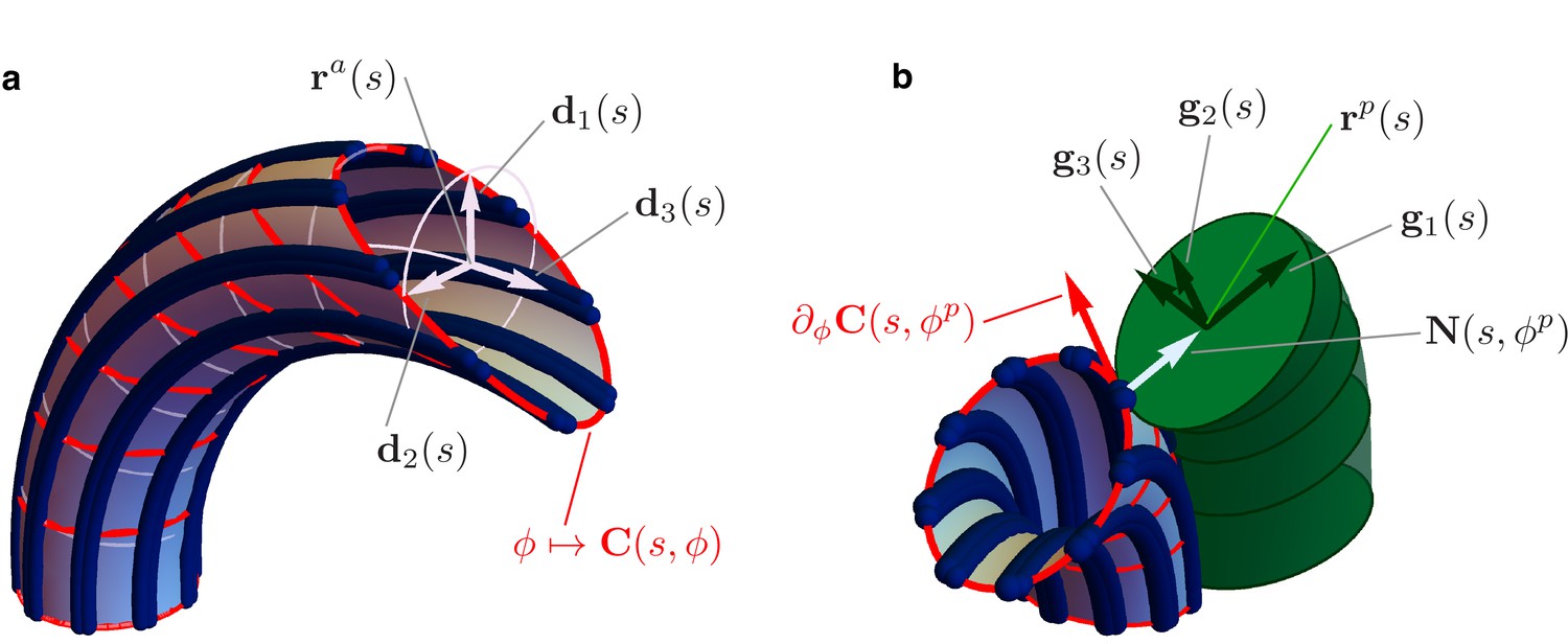
Details of the mechanical model.

(a) Geometry of the Ax. MTs lie on a tubular surface $C (s, ϕ)$ parametrized by generalized polar coordinates $s$ and $ϕ$ , where $s$ is the arc length of the axonemal centerline $𝐫^{a}$ . The unit vectors $𝐝_{1} (s)$ and $𝐝_{2} (s)$ lie on the orthogonal cross sections of the Ax (light blue circles). The material sections of the Ax are given by the curves $ϕ \mapsto 𝐂 (s, ϕ)$ (red), which connect points of neighbouring axonemal MTs corresponding to the same arc length $s$ . Bend deformations of the axoneme are generated by the shear (collective sliding) of MTs. The shear is quantified by the angle between the orthogonal sections and the material sections of the Ax. (b) Geometry of the euglenid flagellum, detail of the Ax-PFR attachment. The unit vectors $𝐠_{1} (s)$ and $𝐠_{2} (s)$ generate the plane of the PFR’s cross sections. The vector $𝐠_{1} (s)$ is parallel to the outer unit normal to the axonemal surface $𝐍 (s, ϕ^{p})$ , while $𝐠_{2} (s)$ is parallel to the tangent vector to the material section $\partial_{ϕ} 𝐂 (s, ϕ^{p})$ .

Figure 5

Download asset Open asset

Flagellar non-planarity arising from structural incompatibility.

The Ax-PFR mechanical interplay is explained in a three-steps argument (left to right). Consider first the two separated structures in their spontaneous configurations (left). The Ax is bent into a planar arc while the PFR is straight. Then, the PFR is forced to match to the Ax, while the latter is kept in its spontaneous configuration (middle). The attachment constraint induces shear strains in the PFR, such that the composite system cannot be in mechanical equilibrium without external forcing. When the composite system is released (right), it reaches equilibrium by the relaxation of the PFR shear, which induces additional distortion of the Ax. At equilibrium, an optimal energy compromise is reached, which is characterized by an emergent non-planarity.

Figure 6

Download asset Open asset

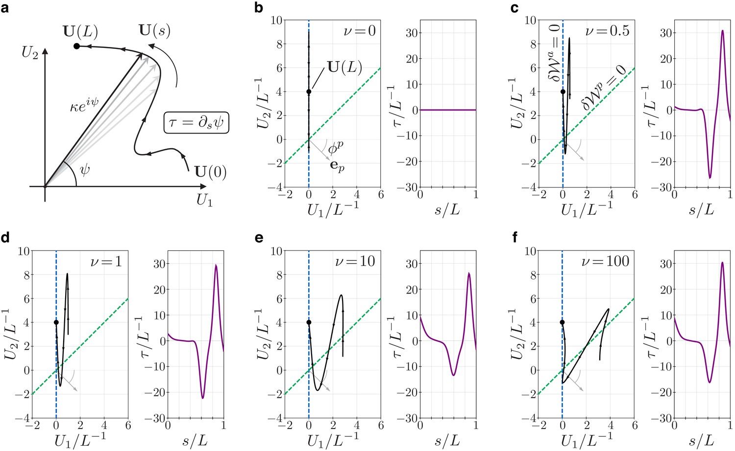
Geometry and mechanics of non-planar flagellar shapes.

(a) The bending vector $𝐔 (s) = (U_{1} (s), U_{2} (s))$ traces a curve on the plane of the bending parameters $U_{1}$ and $U_{2}$ . The norm of the bending vector determines the curvature $κ (s) = | 𝐔 (s) |$ of the flagellum. The rate of change of the angle $ψ (s)$ determines the torsion $τ = \partial_{s} ψ$ . (b–f) Bending vectors’ traces of flagellar equilibrium configurations under the same (steady) dynein actuation, but different values of the material parameter $ν = D^{p} / (B^{a} L^{- 2})$ . Equilibria are minimizer of the energy $𝒲 = 𝒲^{a} + 𝒲^{p}$ . For small values of $ν$ , the Ax component of the energy $𝒲^{a}$ dominates. In this case, $𝐔$ is close to the target bending vector $(0, U_{2}^{*})$ where $U_{2}^{*} (s) = A_{0} + A_{1} \sin (2 π s / L)$ . For large values of $ν$ the PFR component of the energy $𝒲^{p}$ dominates, and equilibria are dragged closer to the line orthogonal to the vector $𝐞_{p}$ (dashed green). The bending vector undergoes rotations which result in torsional peaks of alternating sign.

Figure 6—source code 1 Equilibrium equations solver.: https://cdn.elifesciences.org/articles/58610/elife-58610-fig6-code1-v2.zip
Download elife-58610-fig6-code1-v2.zip

Figure 7

Download asset Open asset

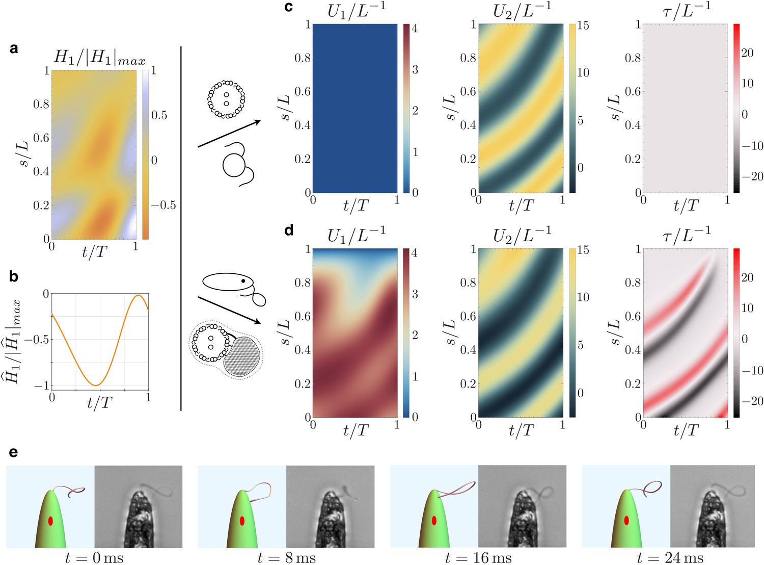
Kinematics of the beating euglenid flagellum: comparison between theoretical model and experiments.

(a-b) Dyneins’ shear forces. (c) Resulting bending strains and torsion for an Ax actuated by the force pattern (a–b), beating in a viscous fluid, and free of extra-axonemal structures. The beat is planar (Chlamydomonas-like). (d) Resulting bending strains and torsion for an euglenid flagellum (composite structure Ax+PFR) actuated by (a–b) and beating in a viscous fluid. The Ax-PFR interaction generates torsional peaks with alternate sign traveling from the proximal to the distal end of the flagellum. (e) Resulting shapes for the euglenid flagellum at different instants within a beat, and comparison with experimental observations.

Figure 7—source code 1 Flagellar dynamics solver and visualization tool.: https://cdn.elifesciences.org/articles/58610/elife-58610-fig7-code1-v2.zip
Download elife-58610-fig7-code1-v2.zip

Figure 8

Download asset Open asset

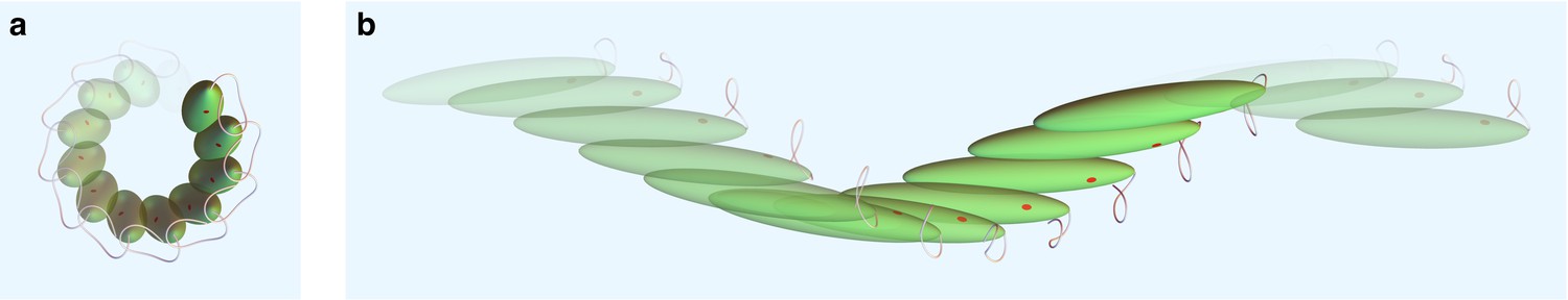
Swimming kinematics.

(a) Side view and (b) top view of swimming cell simulation resulting from the flagellar beat generated by our model. The dimension of the cell body is not to scale with displacements for visualization purposes.

Appendix 1—figure 1

Download asset Open asset

Sketch of two MTs’ centerlines during deformation.

The sliding $σ_{j} (s)$ is defined as the difference between the arc lengths $s$ and $Π_{j} (s)$ . The latter is the arc length corresponding to the projection of $𝐫^{j + 1} (s)$ on the curve $𝐫^{j}$ . We have positive sliding when dyneins push the $j$ -th MT toward the distal end of the flagellum and the $(j + 1)$ -th MT toward the proximal end.

Appendix 3—figure 1

Download asset Open asset

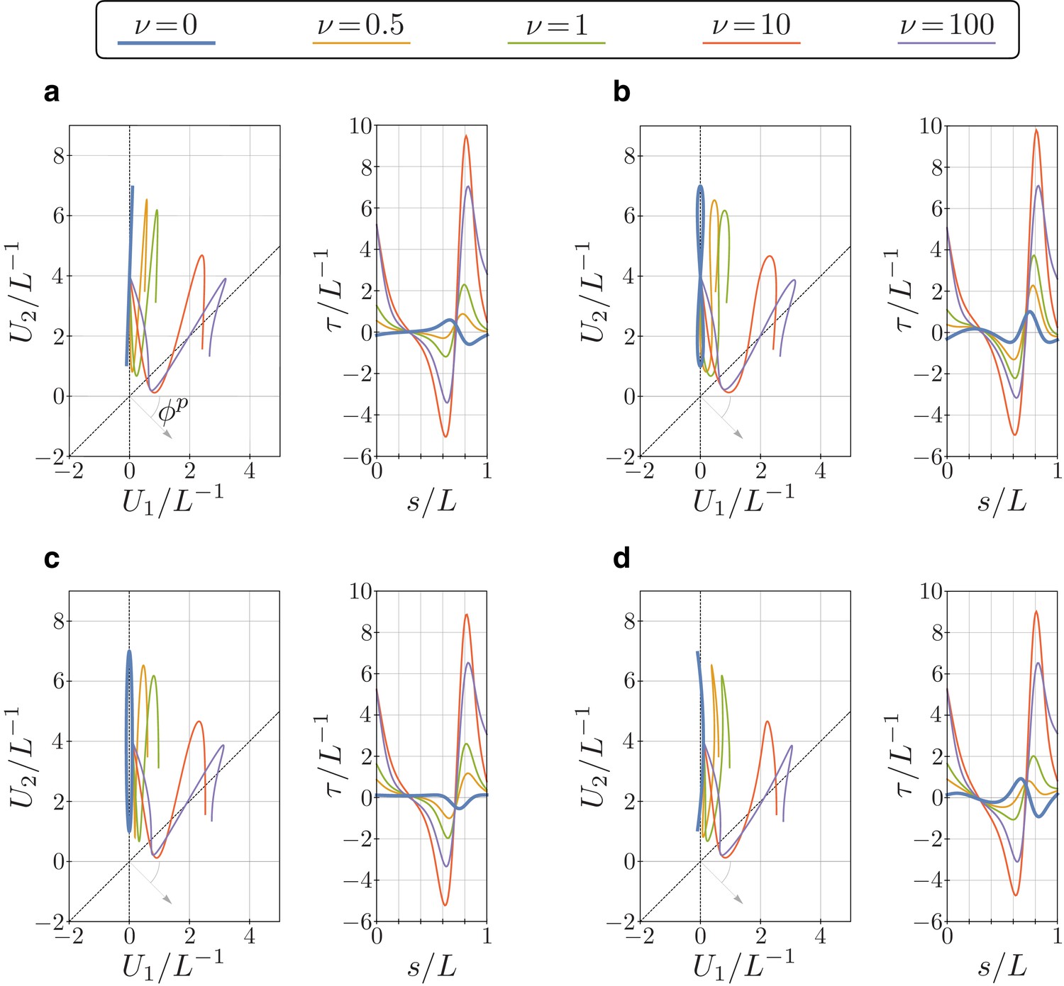
Bending vector traces and torsion of equilibrium configurations of the euglenid flagellum under four different target bending strains, and for different values of the parameter $ν = D^{p} / (B^{a} L^{- 2})$ .

The target bending strains are given by $(u_{1}^{*}, u_{2}^{*})$ , with $u_{2}^{*} (x) = a_{0} + a_{1} \sin (2 π x)$ and $u_{1}^{*} = ϵ {\tilde{u}}_{1}^{*}$ , where (a) ${\tilde{u}}_{1}^{*} (x) = \sin (2 π x)$ , (b) ${\tilde{u}}_{1}^{*} (x) = \sin (4 π x)$ , (c) ${\tilde{u}}_{1}^{*} (x) = \cos (2 π x)$ , and (d) ${\tilde{u}}_{1}^{*} (x) = \cos (4 π x)$ .

Appendix 5—figure 1

Download asset Open asset

Swimming kinematics: numerical results.

(a) Cell body and body frame unit vectors. (b) Body velocity and (c) rotational velocity projections on the body frame vectors during a flagellar beat.

Appendix 5—figure 1—source code 1 Swimming dynamics solver.: https://cdn.elifesciences.org/articles/58610/elife-58610-app5-fig1-code1-v2.zip
Download elife-58610-app5-fig1-code1-v2.zip

Videos

Video 1

Download asset

posterframe for video — Four views of a capillary-trapped specimen of E. gracilis recorded during periodic flagellar beating.

Video 2

Download asset

posterframe for video — Comparison between observations of a beating euglenid flagellum and the numerical simulations of our mechanical model.

Video 3

Download asset

posterframe for video — Simulations of swimming cell kinematics resulting from the flagellar beat generated by our model.

Additional files

Transparent reporting form: https://cdn.elifesciences.org/articles/58610/elife-58610-transrepform-v2.docx
Download elife-58610-transrepform-v2.docx
Appendix 5—figure 1—source code 1 Swimming dynamics solver.: https://cdn.elifesciences.org/articles/58610/elife-58610-app5-fig1-code1-v2.zip
Download elife-58610-app5-fig1-code1-v2.zip

Download links

A two-part list of links to download the article, or parts of the article, in various formats.

Downloads (link to download the article as PDF)

Article PDF

Open citations (links to open the citations from this article in various online reference manager services)

Mendeley

Cite this article (links to download the citations from this article in formats compatible with various reference manager tools)

Giancarlo Cicconofri
Giovanni Noselli
Antonio DeSimone

(2021)

The biomechanical role of extra-axonemal structures in shaping the flagellar beat of Euglena gracilis

eLife 10:e58610.

https://doi.org/10.7554/eLife.58610

Sign up for email alerts

Privacy notice