GWAS of three molecular traits highlights core genes and pathways alongside a highly polygenic background
- Department of Genetics, Stanford University, United States
- Department of Chemical and Systems Biology, Stanford University, United States
- Department of Biomedical Data Sciences, Stanford University, United States
- Department of Biology, Stanford University, United States
Figures
Figure 1 with 1 supplement
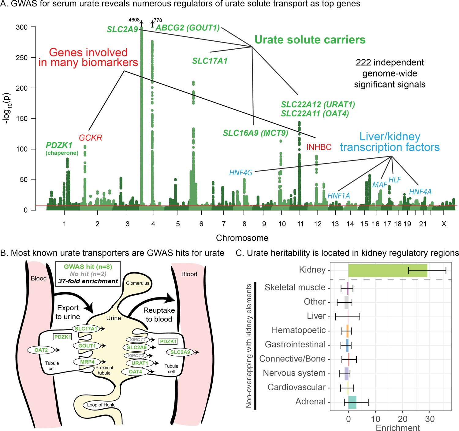
Genetic basis of serum urate variation.
(A) Genome-wide associations with serum urate levels in the UK Biobank. Candidate genes that may drive the most significant signals are indicated; in most cases in the paper, the indicated genes are within 100 kb of the corresponding lead SNPs. (B) Eight out of 10 genes that were previously annotated as being involved in urate transport (Wright et al., 2010; Anzai et al., 2007) are within 100 kb of a genome-wide significant signal. The signal at MCT9 is excluded from figure and enrichment due to its uncertain position in the pathway (Fisel et al., 2018). (C) Urate SNP-based heritability is highly enriched in kidney regulatory regions compared to the genome-wide background (analysis using stratified LD Score regression). Other tissues show little or no enrichment after removing regions that are active in kidney. See Figure 1—figure supplement 1 for the uncorrected analysis.
Figure 1—figure supplement 1
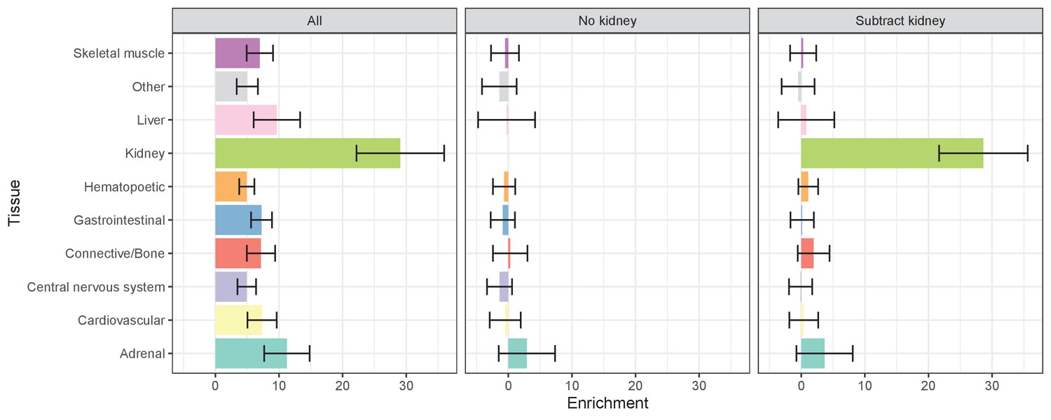
Estimates of serum urate SNP-based heritability within cell and tissue group annotations using LD Score regression (Finucane et al., 2015).
Conditions represent naive multiple regression against all cell types simultaneously (left), multiple regression of non-kidney cell types after removing regions overlapping with kidney (middle), and multiple regression of non-kidney cell types excluding kidney regions along with the original kidney annotation (right). 95% confidence intervals are shown. The latter two results suggest that almost none of the urate SNP-based heritability lies specifically within any non-kidney cell type.
Figure 2
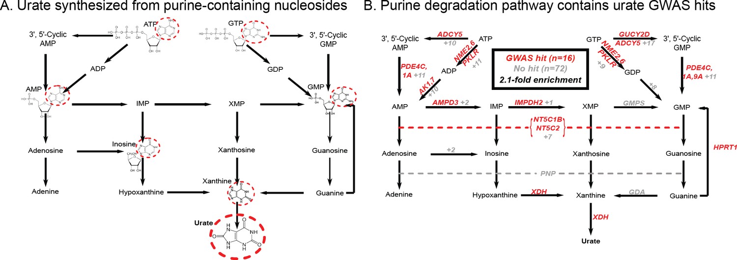
Modest enrichment of signals among genes involved in urate biosynthesis.
(A) Urate is a byproduct of the purine biosynthesis pathway. The urate component of each molecule is highlighted. (B) The same pathway indicating genes that catalyze each step. Genes with a genome-wide significant signal within 100 kb are indicated in red; numbers in gray indicate the presence of additional genes without signals. Pathway adapted from KEGG.
Figure 3 with 5 supplements

Genetic basis of IGF-1 variation.
Manhattan plot showing the locations of major genes associated with IGF-1 levels in the IGF-1 pathway (yellow), transcription factor (blue), pleiotropic gene (red), or unknown function (black) genes sets.
Figure 3—figure supplement 1
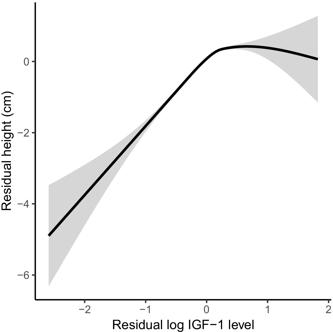
Covariate-adjusted IGF-1 levels are significantly associated with covariate-adjusted height in UK Biobank.
Figure 3—figure supplement 2
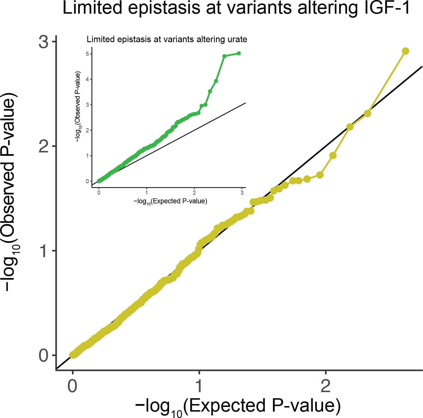
QQ-plot testing for epistasis plots all pairs of lead variants with for IGF-1 levels (Materials and methods).
Inset is the corresponding plot for urate levels.
Figure 3—figure supplement 3
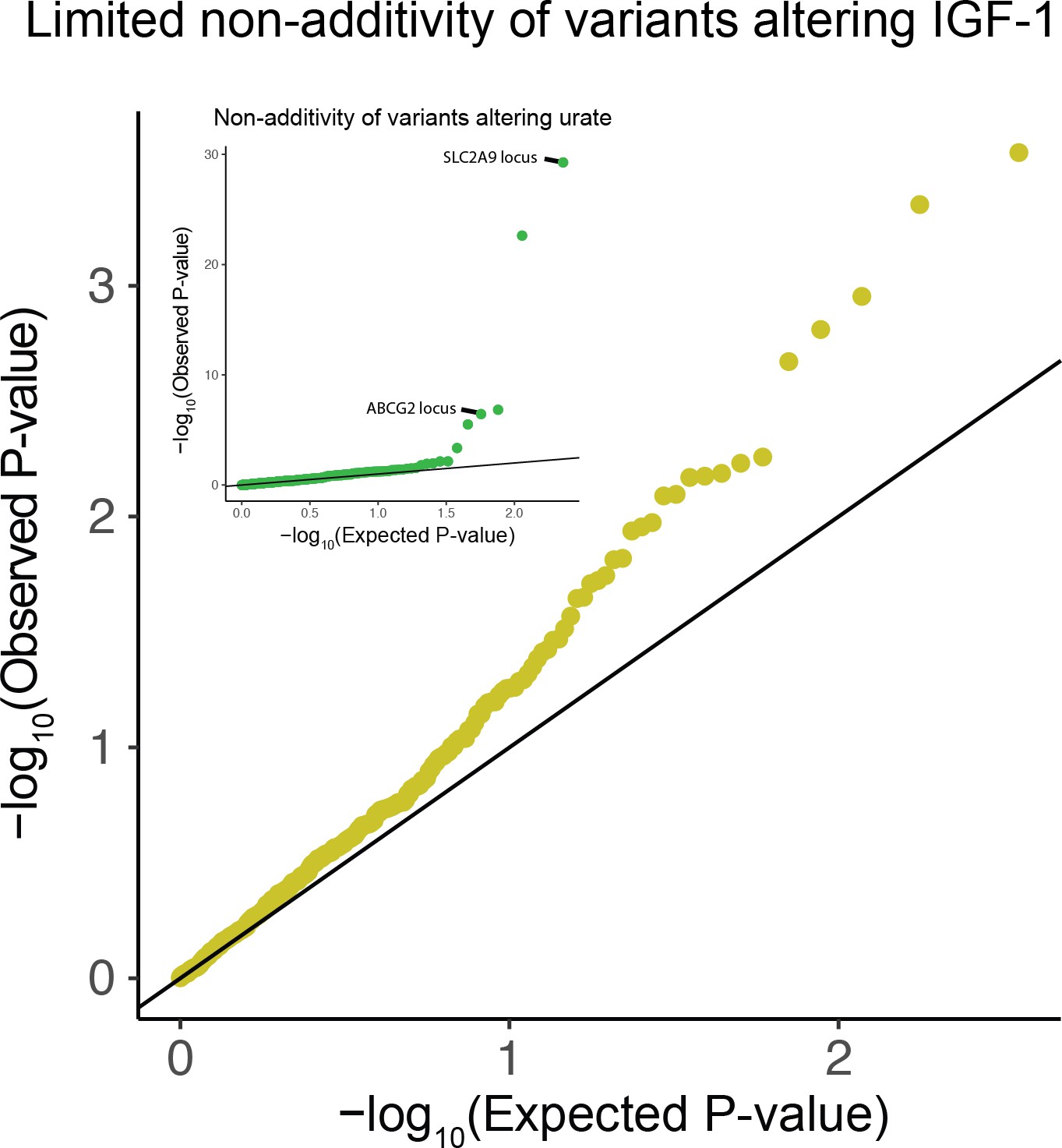
QQ-plot testing for non-additivity at IGF-1 associated SNPs.
All lead variants with passing quality control were tested for departures from an additive model (Materials and methods). Inset is the same analysis run on associations with serum urate levels.
Figure 3—figure supplement 4
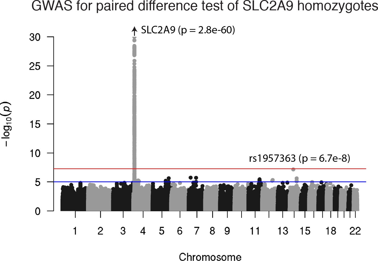
A genome-wide association study for paired differences in effect size by SLC2A9 genotype.
Other than at the SLC2A9 locus, there are no genome-wide significant differences.
Figure 3—figure supplement 5
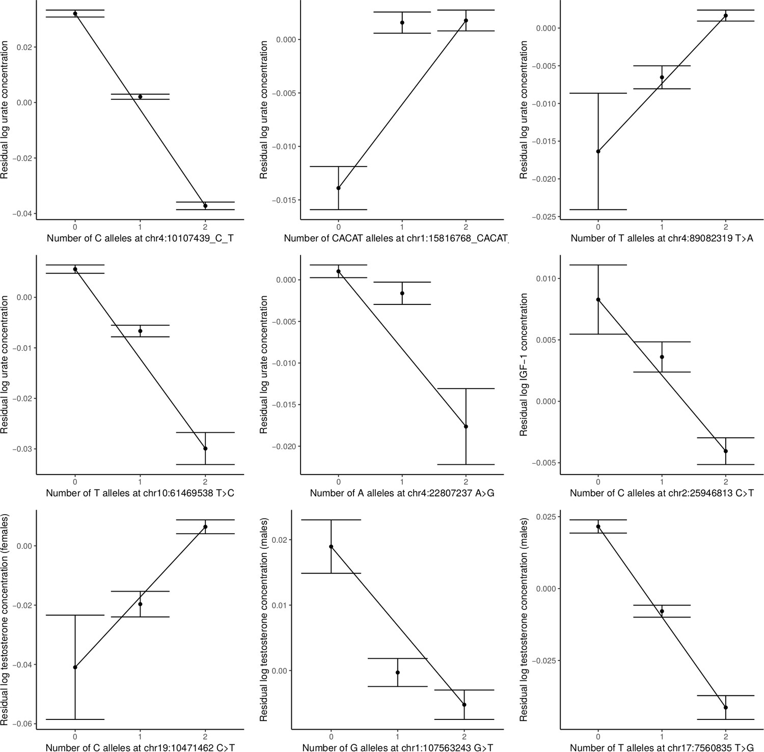
Non-additivity in serum urate concentrations at chr4:10107439 C>T, chr1:15816768 CACAT>C, chr4:89082319 T>A, chr4:22807237 A>G, and chr10:61469538 T>A; at chr2:25946813 C>T in IGF-1; and in female testosterone at chr19:10471462 C>T and male testosterone at chr1:107563243 G>T and chr17:7560835 T>G.
95% confidence intervals shown, and lines are drawn between homozygotes. Only chr1:15816768 CACAT>C, chr1:107563243 G>T, and chr4:22807237 A>G show substantial departure from additivity (revealing a recessive effect in all three cases).
Figure 4
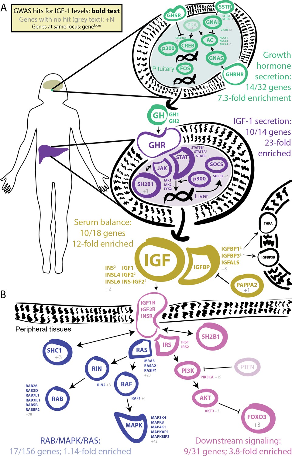
GWAS hits in the IGF-1 pathway.
Bolded and colored gene names indicate that the gene is within 100 kb of a genome-wide signficant hit. Gray names indicate absence of a genome-wide signficant hit; gray numbers indicate that multiple genes in the same part of the pathway with no hit. Superscript numbers indicate that multiple genes are located within the same locus and hence may not have independent hits. (A) Upstream pathway that controls regulation of IGF-1 secretion into the bloodstream. (B) Downstream pathway that controls regulation of IGF-1 response.
Figure 5 with 1 supplement
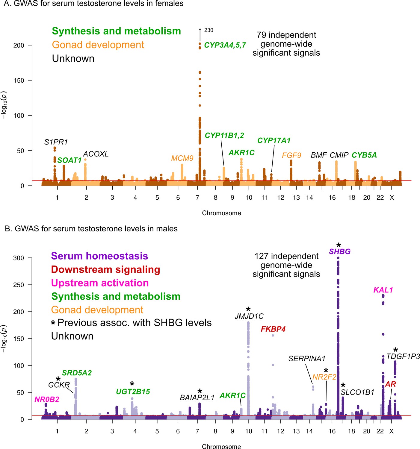
Manhattan plots for testosterone.
(A) Females. (B) Males. Notice the low overlap of lead signals between females and males. FAM9A and FAM9B have been previously proposed as the genes underlying the KAL1 locus (Ohlsson et al., 2011).
Figure 5—figure supplement 1
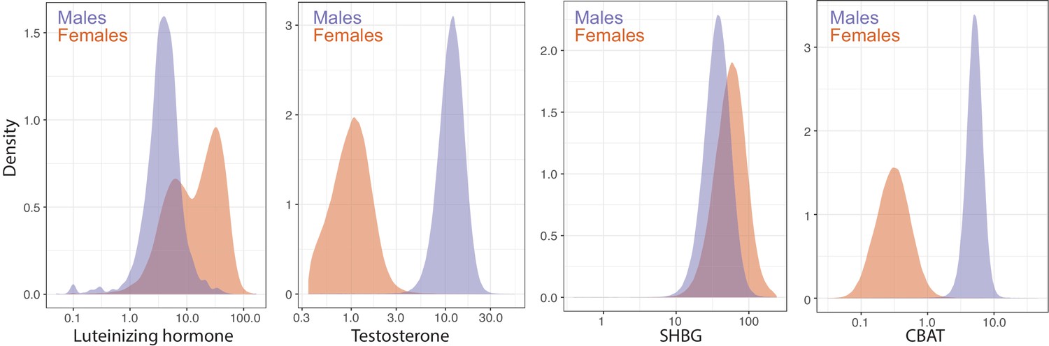
Distributions of female and male luteinizing hormone, testosterone, sex hormone binding globulin (SHBG), and calculated bioavailable testosterone (CBAT) levels in the UK Biobank.
Luteinizing hormone is from primary care records (Materials and methods), while Testosterone, SHBG, and CBAT are measured or derived from the baseline assessment center visit.
Figure 6 with 2 supplements
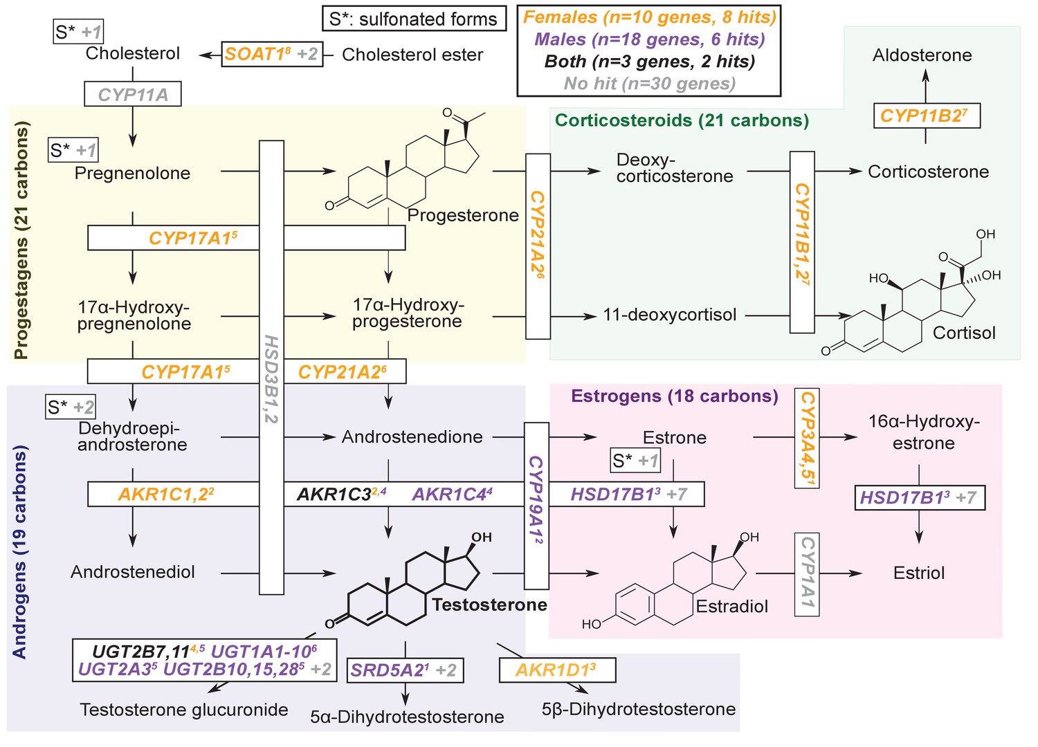
Pathway diagram for steroid hormone biosynthesis showing GWAS hits for females and males.
The text color indicates genes within 100 kb of a genome-wide significant hit for females (orange), males (blue), or both females and males (black). Gray gene names or numbers indicates genes with no hits. Colored superscripts indicate multiple genes from the same locus (and hence may reflect a single signal). ‘S*’ indicates that an additional, sulfonated metabolite, along with the catalytic step and enzymes leading to it, is not shown. Pathway from KEGG; simplified based on a similar diagram in Wikipedia, 2012.
Figure 6—figure supplement 1
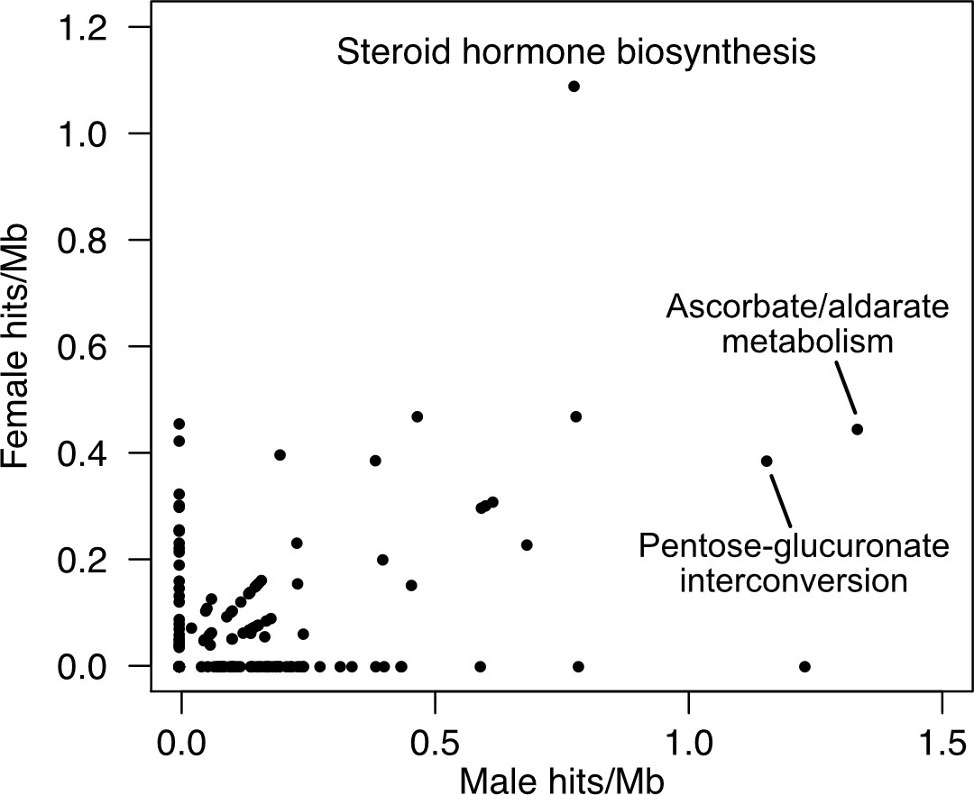
The KEGG pathway for steroid hormone biosynthesis is enriched for hits in both female and male testosterone GWAS.
The enrichments for male hits in ‘Ascorbate/aldarate metabolism’ and ‘Pentose-glucuronate interconversion’ are almost entirely driven by the UGT genes, which are part of ‘Steroid hormone biosynthesis’.
Figure 6—figure supplement 2
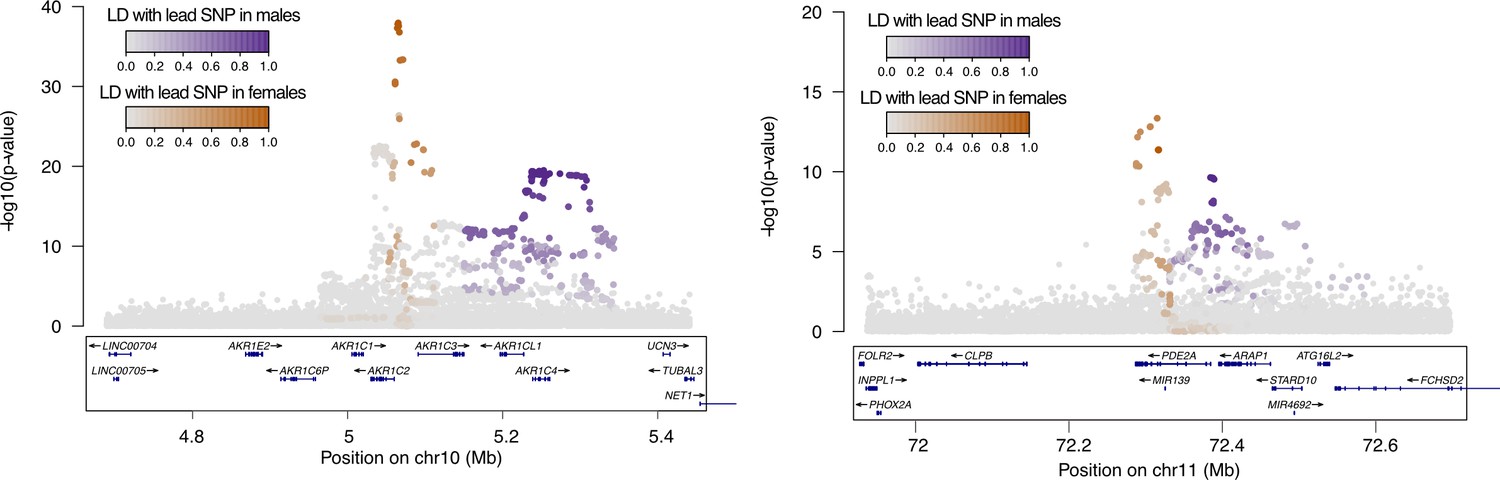
Non-overlapping female and male GWAS signals at AKR1C (left) and PDE2A (right) loci.
Figure 7 with 5 supplements
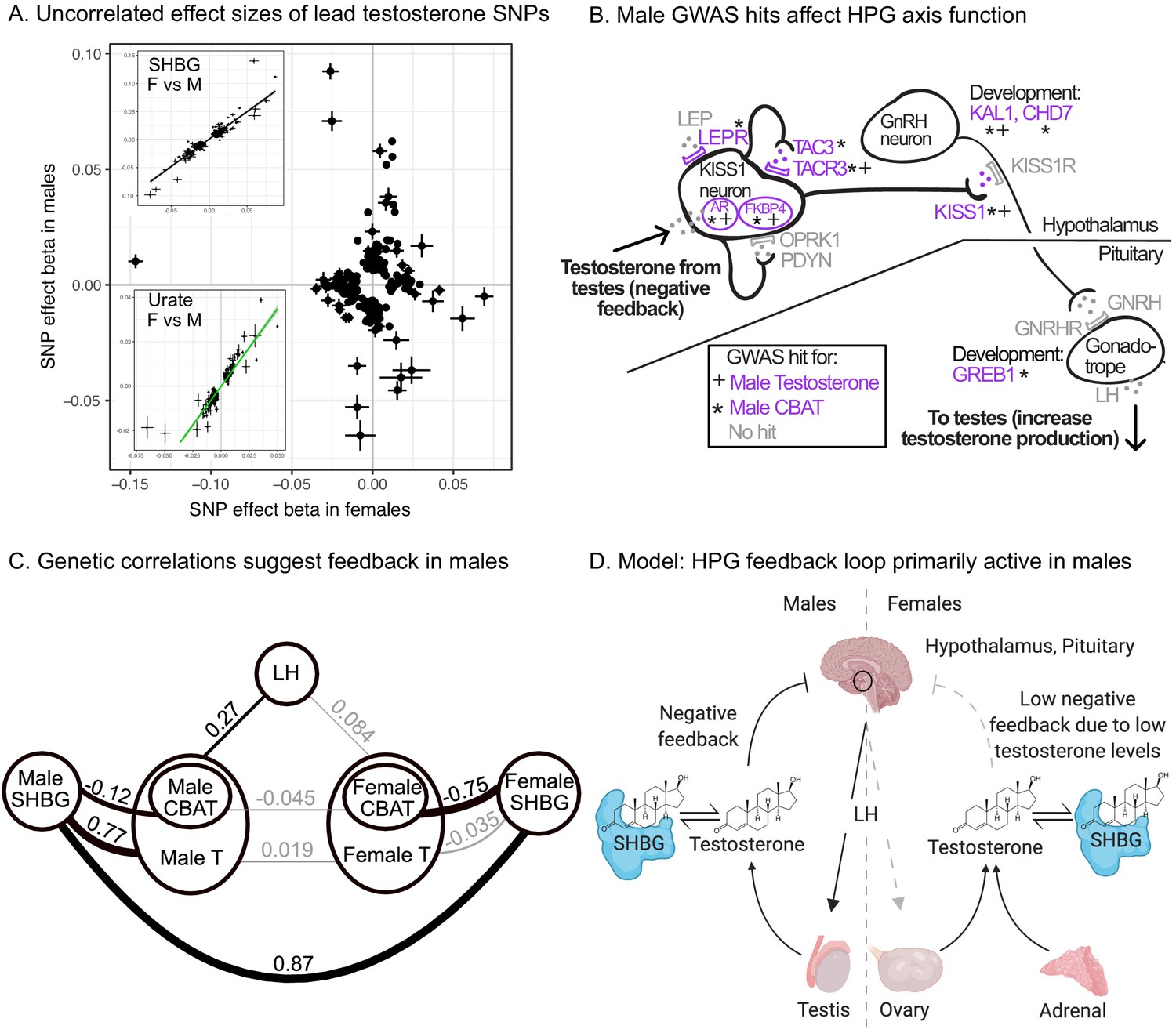
Sex differences in genetic variation in testosterone.
(A) When comparing lead SNPs (p<5e-8 ascertained in either females or males), the effects are nearly non-overlapping between females and males. Other traits show high correlations for the same analysis (see urate and SHBG in inset). (B) Schematic of HPG axis signaling within the hypothalamus and pituitary, with male GWAS hits highlighted. These variants are not significant in females. (C) Global genetic correlations, between indicated traits (estimated by LD Score regression). Thickness of line indicates strength of correlation, and significant (p<0.05) correlations are in bold. Note that LH genetic correlations are not sex-stratified due to small sample size in the UKBB primary care data (N = 10,255 individuals). (D) Proposed model in which the HPG axis and SHBG-mediated regulation of testosterone feedback loop is primarily active in males. Abbreviations for all panels: SHBG, sex hormone-binding globulin; CBAT, calculated bioavailable testosterone; LH, luteinizing hormone.
Figure 7—figure supplement 1
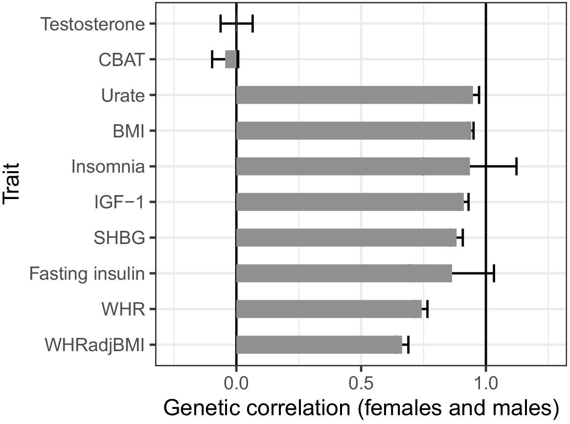
Genetic correlations between females and males across select traits.
Both testosterone and calculated bioavailable testosterone (CBAT) show very little genetic correlation, in stark contrast to most other complex traits.
Figure 7—figure supplement 2
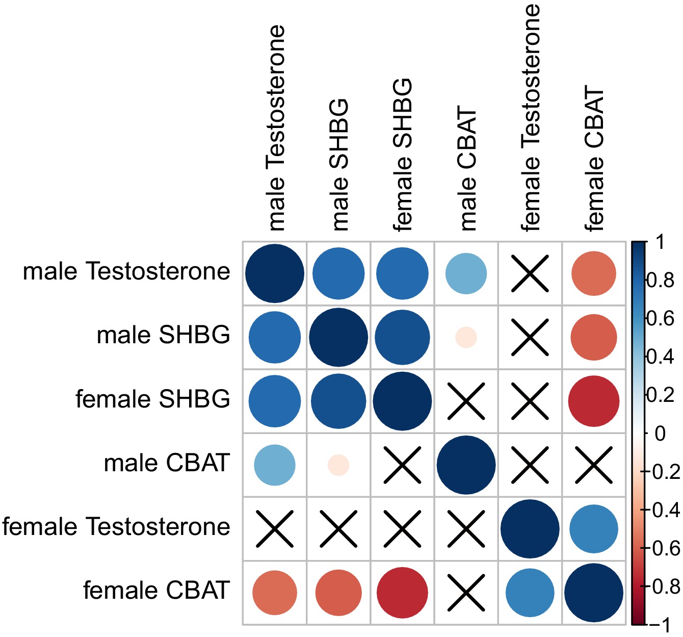
Genetic correlations (estimated by LD Score Regression) between total testosterone, SHBG, and calculated bioavailable testosterone (CBAT) in females and males.
‘X’ indicates a non-significant genetic correlation.
Figure 7—figure supplement 3
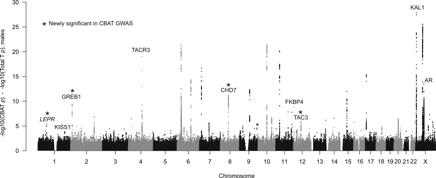
Manhattan plot of difference in significance of assocation comparing GWAS of calculated bioavailable testosterone (CBAT) to total testosterone.
Only points more significant in CBAT GWAS (i.e. positive values on y-axis) are shown. Genes with known roles in the HPG axis are annotated.
Figure 7—figure supplement 4
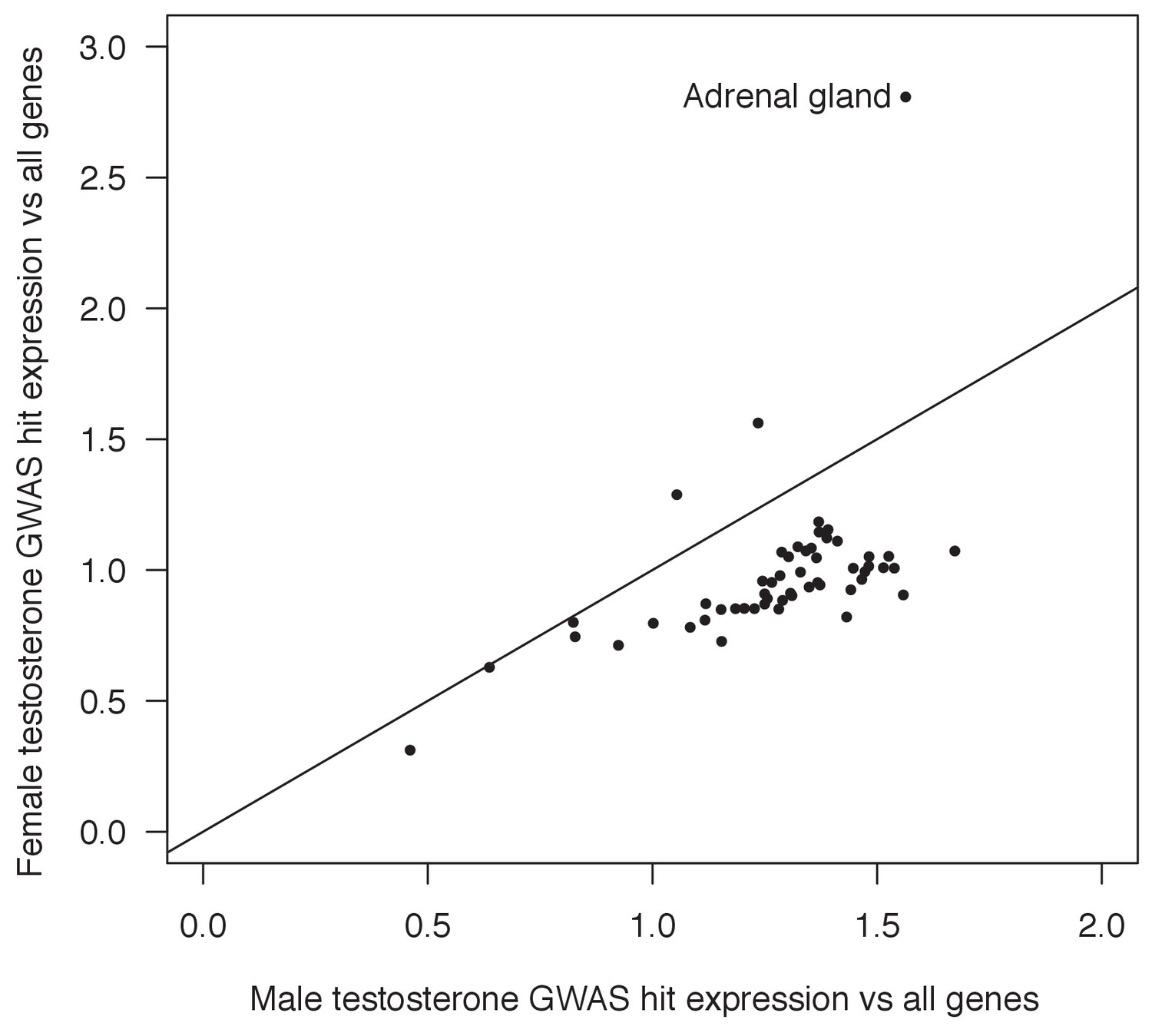
Mean expression of testosterone GWAS hits in females or males (defined as mean log-transformed counts of hits divided by mean log-transformed counts of all genes) in each of 48 GTEx tissues.
Figure 7—figure supplement 5
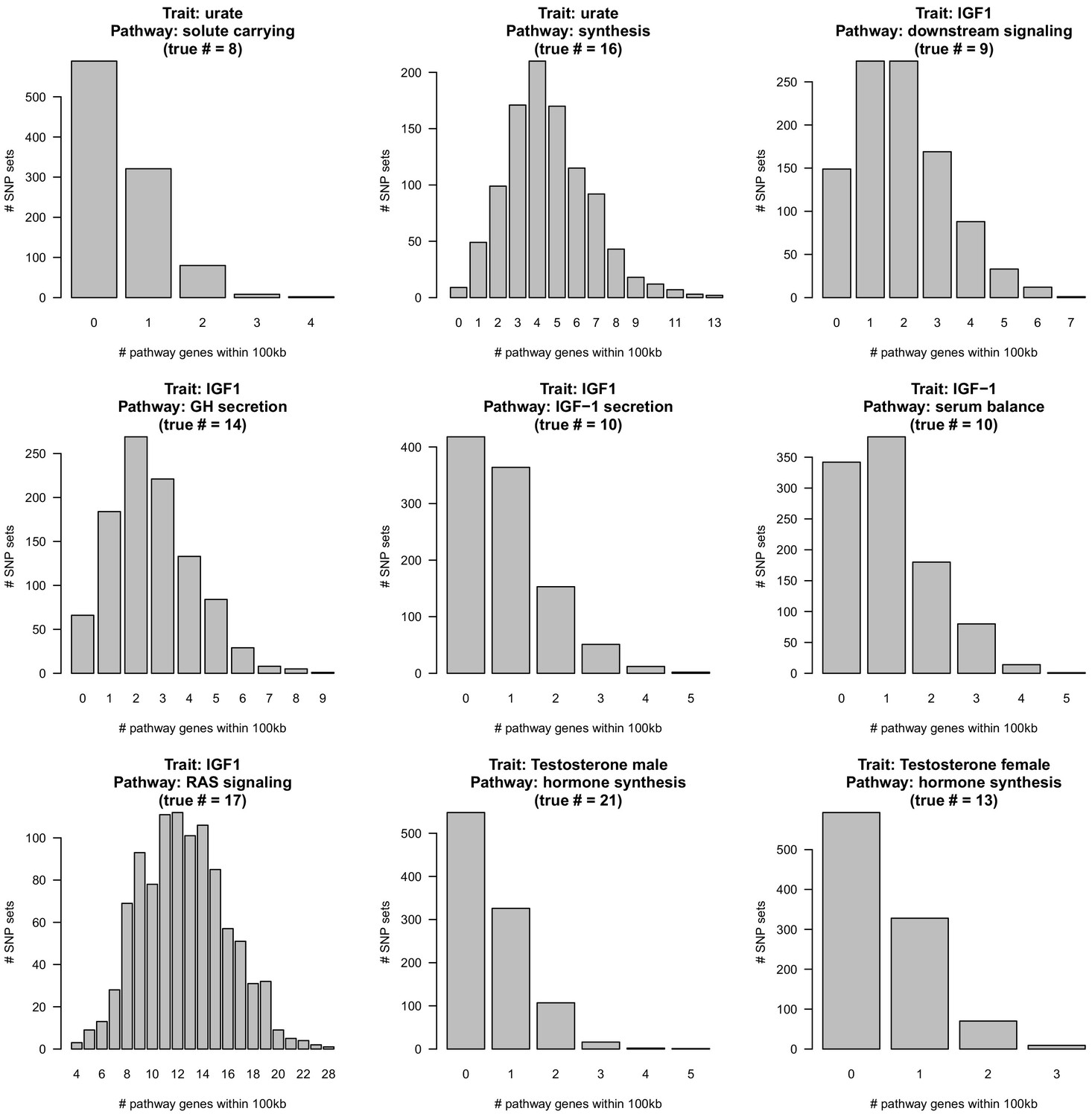
Enrichment of random matched SNPs in core pathways.
For each GWAS indicated, 1000 sets of equally-sized random SNPs matched to GWAS SNPs for LD, allele frequency, and genic distance (see Materials and methods) were overlapped with the indicated core pathway with 100 kb windows. The.
Figure 8 with 14 supplements

Despite clear enrichment of core genes and pathways, most SNP-based heritability for these traits is due to the polygenic background.
(A) Cumulative distribution of SNP-based heritability for each trait across the genome (estimated by HESS). The locations of the most significant genes are indicated. Insets show the fractions of SNP-based heritability explained by the most important genes or pathways for each trait. (B) Estimated fractions of SNPs with non-null associations, in bins of LD Score (estimated by ashR). Each point shows the ashR estimate in a bin representing 0.1% of all SNPs. The inset text indicates the estimated fraction of variants with a non-null marginal effect, that is, the fraction of variants that are in LD with a causal variant. (C) Simulated fits to the data from (B). X-axis truncated for visualization as higher LD Score bins are noisier. Simulations assume that of SNPs have causal effects drawn from a normal distribution centered at zero (see Materials and methods). The simulations include a degree of spurious inflation of the test statistic based on the LD Score intercept. Other plausible assumptions, including clumpiness of causal variants, or a fatter-tailed effect distribution would increase the estimated fractions of causal sites above the numbers shown here.
Figure 8—figure supplement 1
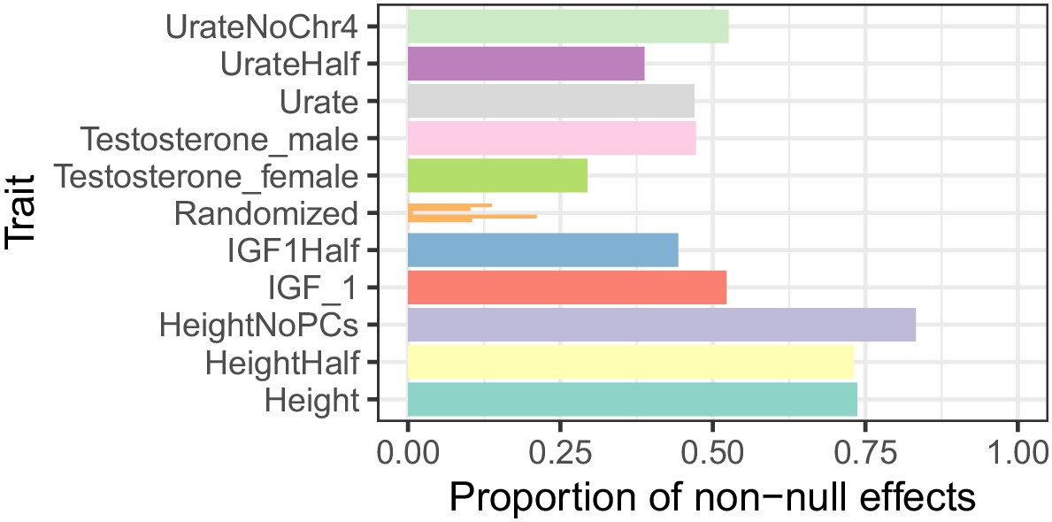
Proportion of non-null associations in a random sample of 100,000 variants for each trait.
Variants are then filtered to those with minor allele frequency greater than 5%, and ashR is run on the beta and standard error to estimate the proportion of non-null associations. ‘‘UrateNoChr4’’ is the Urate GWAS with chromosome 4 excluded, where the two largest effect loci, SLC2A9 and ABCG2, are both located. Traits with the suffix ‘Half’ are 50% downsamplings of the White British cohort to approximate the sample sizes of the sex-stratified testosterone GWAS. ‘Randomized’ are random associations generated by evaluating shuffled versions of the Urate (n = 3 shuffles) and IGF-1 (n = 3 shuffles) phenotypes and represent estimates we might expect under the null distribution of no associations, where we observe some noise but consistently observe estimates well below that of un-shuffled traits. These global estimates represent the proportion of all variants in a given trait that are linked to causal sites.
Figure 8—figure supplement 2
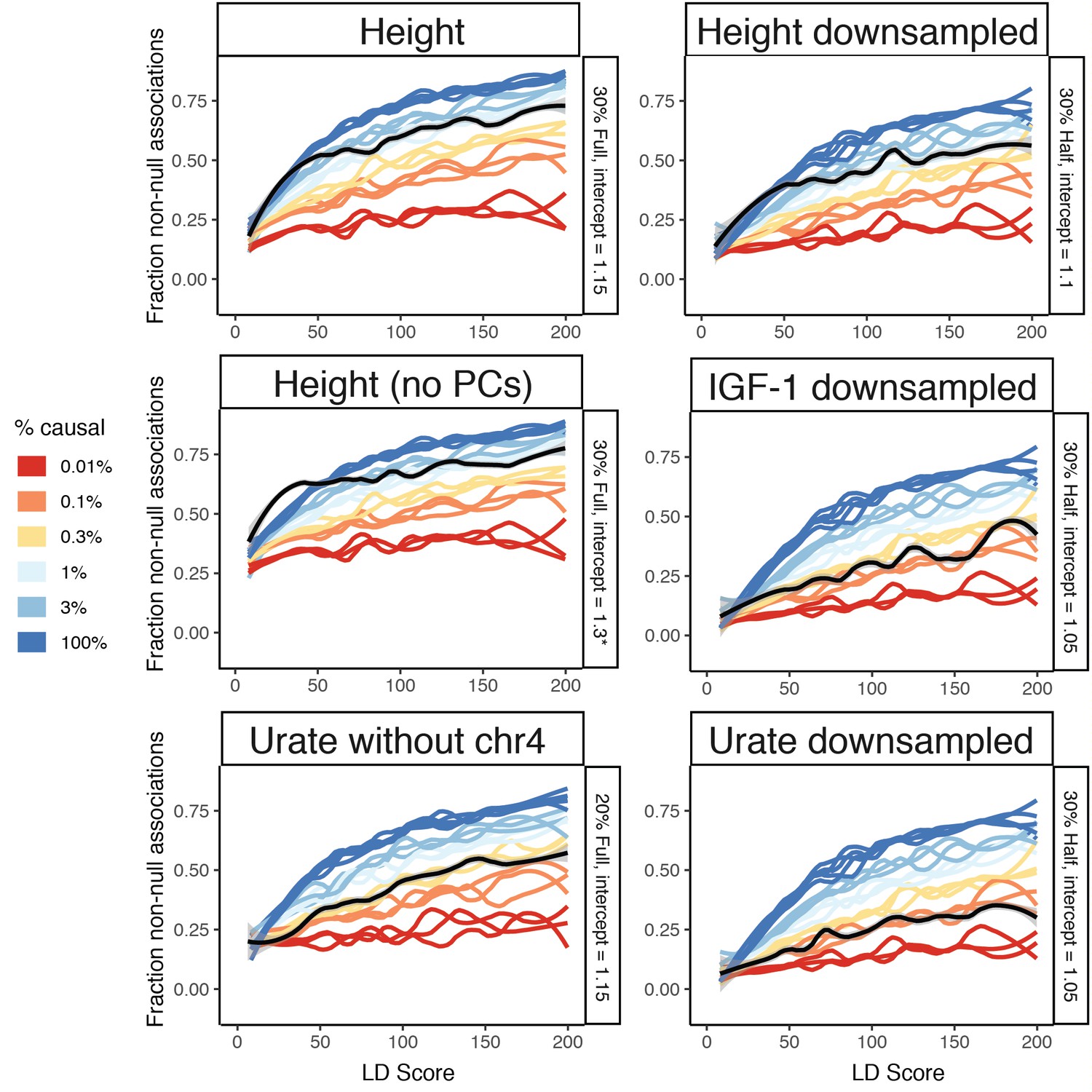
Additional traits to fit causal simulations on.
Height, height without principal components regressed out of the GWAS, Urate with chromosome four excluded (where both SLC2A9 and ABCG2 are located, reducing SNP-based heritability to ≈20%), and random 50% downsamplings of height, IGF-1, and urate (including chromosome 4) are shown. See Figure 8—figure supplement 3 for additional sex hormone traits. Despite matching simulations for sample size, slight reductions in causal variant count are still observed in downsampled traits, suggesting that power is still possibly limiting, of particular relevance to the sex-stratified testosterone GWAS. As expected, excluding principal components from the GWAS dramatically increases the intercept. * 1.3 was the highest tested intercept and is still too low, but no more runs were completed as the curve is clearly shaped very differently than simulation runs regardless of intercept. We recommend performing GWAS while regressing out principal components to avoid difficult to interpret results. See Figure 8—figure supplement 3 for additional fits to sex hormone related traits.
Figure 8—figure supplement 3
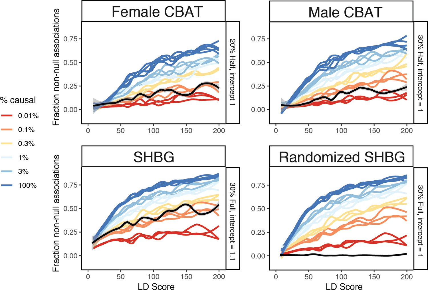
Prediction plots for the causal SNP counts underlying calculated bioavailable testosterone (CBAT) in females and males, as well as sex hormone binding globulin (SHBG) and a randomized version of SHBG.
CBAT traits are similar to their testosterone counterparts and SHBG is estimated to have slightly more causal variants (≈0.2%).
Figure 8—figure supplement 4
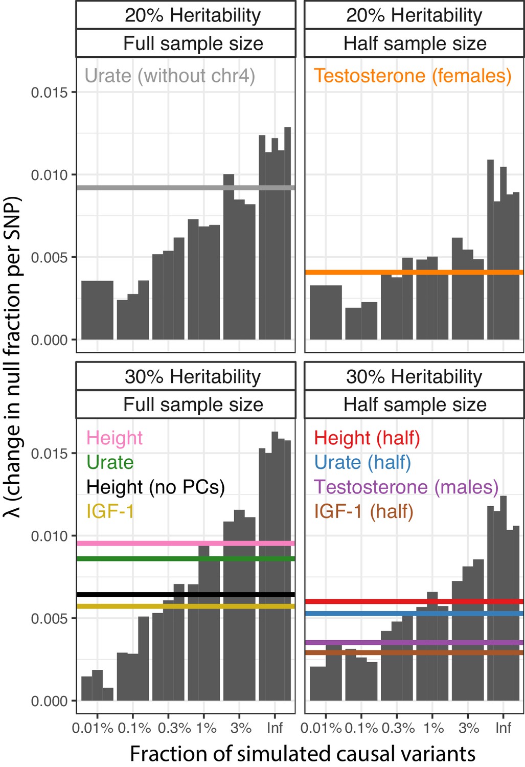
Parametric causal fraction on LD Scores reproduces SNP-based heritability-based estimates.
For each study sample size (Full, full UK Biobank White British; Half, 50% downsample [and sex-stratified]) and SNP-based heritability (20% or 30%), simulations run with different causal variant proportions (n = 3 reps except infinitesimal, n = 5) were used as a background to estimate the causal site proportions for each complex trait. Complex trait non-linear least squares λ estimates are shown as horizontal lines.
Figure 8—figure supplement 5
Estimates of causal sites are conservative with respect to SNP concentration within the genome.
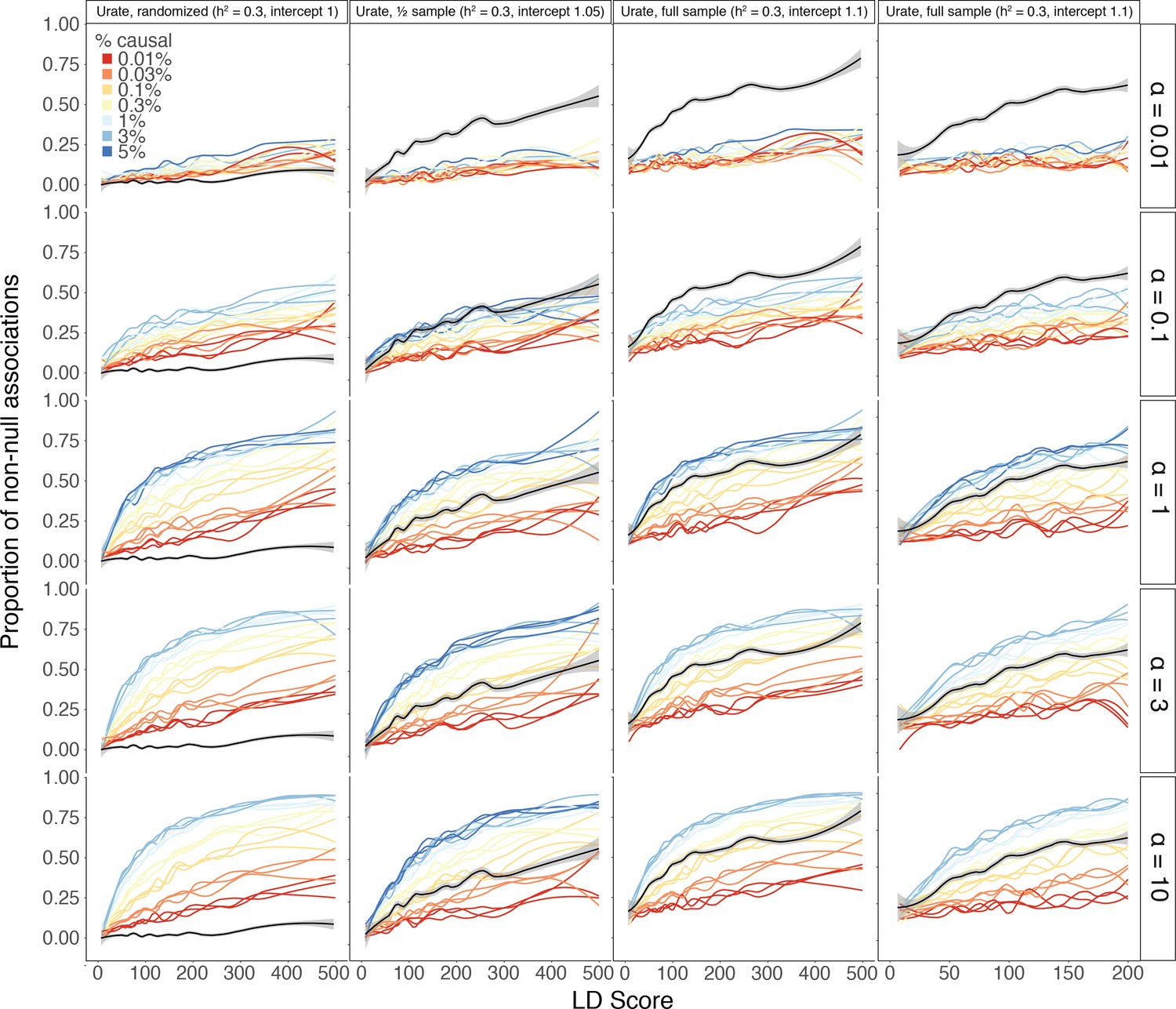
Rather than drawing SNPs uniformly at random from those with MAF >1% (Materials and methods), instead each megabase window was assigned a distinct probability ρ of SNPs being causal within that megabase window. For a given causal fraction c, ρ was drawn at random from . Thus, the mean causal fraction across all megabase windows in the genome is still c, and this fraction is concentrated more in single windows under decreasing values of α. The standard results shown in main text correspond to . As we decrease α, the estimates consistently increases, regardless of the same size or LD Score axis threshold. However, the results consistently stay above the randomized version of the trait, suggesting that the estimates remain non-zero even for very concentrated SNP-based heritability.
Figure 8—figure supplement 6
Effect of distribution of causal site betas on estimates of causal variant count.
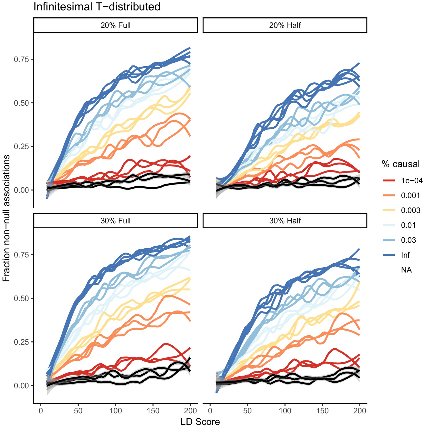
A model where every variant in the genome is drawn from a one-degree-of-freedom T-distribution is shown in black across the different heritabilities and samples sizes. Because some small number of variants have very large effects in the T-distribution, and the total SNP-based heritability is normalized to this additional variance, the estimate is downward biased and suggests that rather than 100% of variants being causal, instead less than 0.01% are causal. In practice, most effect sizes are not as overdispersed as a T-distribution, although some traits (e.g. Urate) have a few variants with very large effect.
Figure 8—figure supplement 7
Association between minor allele frequency and estimated proportion of causal variants.
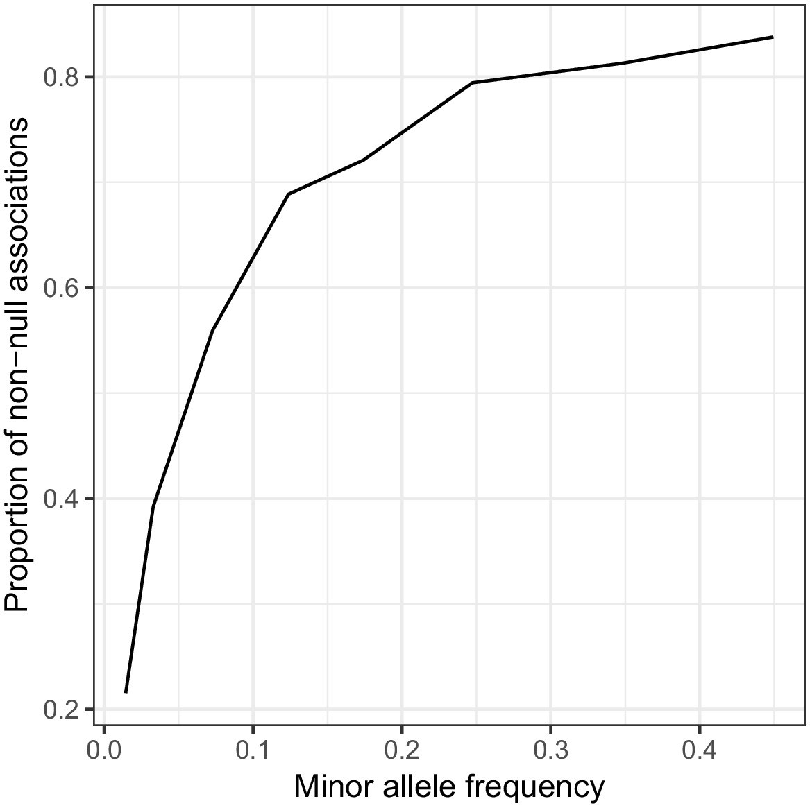
Simulated traits were generated with every variant with MAF >1% being causal (with effect size drawn from N(0,1) independently) and a GWAS was performed with . Then, for each MAF bin, 100,000 variants were sampled at random, and ashR was run to estimate the proportion of causal variants (or variants in LD with a causal variant) within each bin. There is a strong relationship with minor allele frequency, suggesting that power might still be a consideration even at UK Biobank sample sizes. See also Figure 8—figure supplement 8.
Figure 8—figure supplement 8
Effect of minor allele frequency cutoff on the estimates obtained.
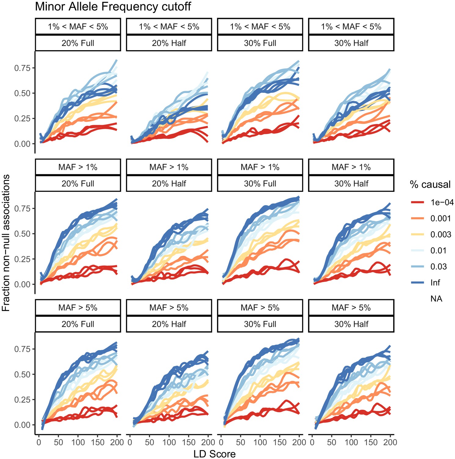
Three choices are considered – MAF >1%, MAF >5%, and MAF between 1% and 5%. There is some attenuation of the estimates in the MAF between 1% and 5% analysis, and the infinitesimal estimates are below that of the models with fewer causal sites, supporting the notion that power is still limiting.
Figure 8—figure supplement 9
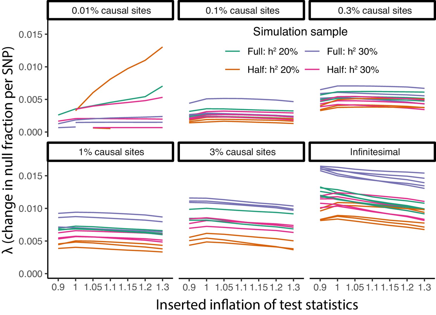
Parametric causal fraction is robust to population structure.
Within each causal site proportion (faceted), inflation added by systematically reducing standard errors was applied with ratios 0.9 through 1.3. For each, the parametric λ fit was calculated using non-linear least squares (Materials and methods). Across this range of inflation levels, there was no large or consistent change in λ estimates, suggesting the λ fit is relatively robust to population structure.
Figure 8—figure supplement 10
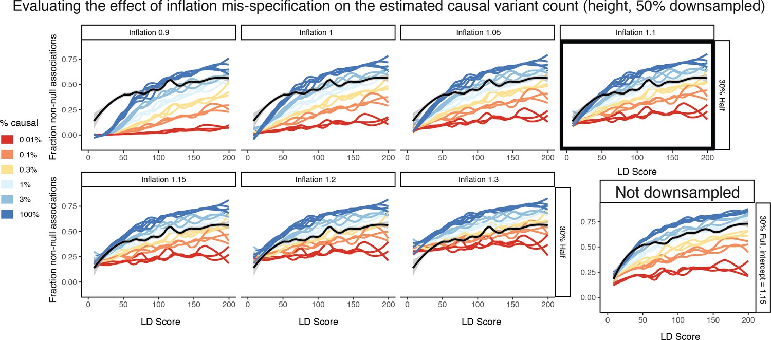
Estimating the effect of inflation mis-specification on the estimated causal variant count.
50% downsampled height is used as an example. When changing the inflation, dramatic differences in the best fitting curve are possible in the simulation matching approach, ranging from greater than 3% at an inflation of 0.9 to around 0.2% for an inflation of 1.3. This is in part exacerbated by the reduced difference between the simulations with different causal percentages at high inflation levels. The best intercept is chosen on the basis of the closest fit at an LD Score of 0 (selected in black box, intercept = 1.1). Note that sample size can change this intercept for the same trait, as shown by the full sample height results (where best intercept = 1.15). However, the resulting estimate is the very similar conditional on intercept.
Figure 8—figure supplement 11
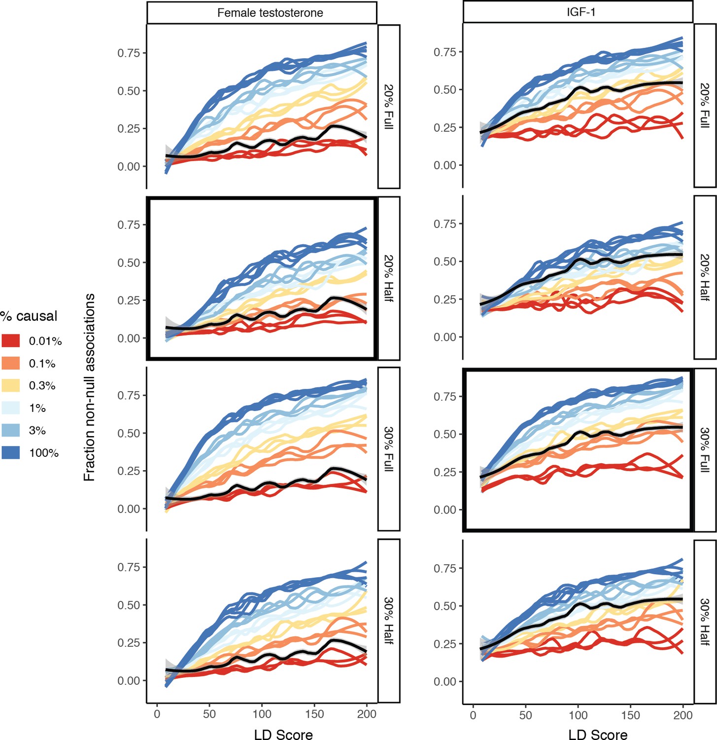
Effect of mis-specification of SNP-based heritability or sample size in the simulation matching approach.
For female testosterone (left) and IGF-1 (right), the correct specification that corresponds to the trait is selected in black. All other estimates are given as well, revealing that the choice of SNP-based heritability and sample size does have a moderate effect on the resulting estimates. As such, we recommend matching the sample size and SNP-based heritability of the simulation GWAS as closely as possible to the traits under study.
Figure 8—figure supplement 12
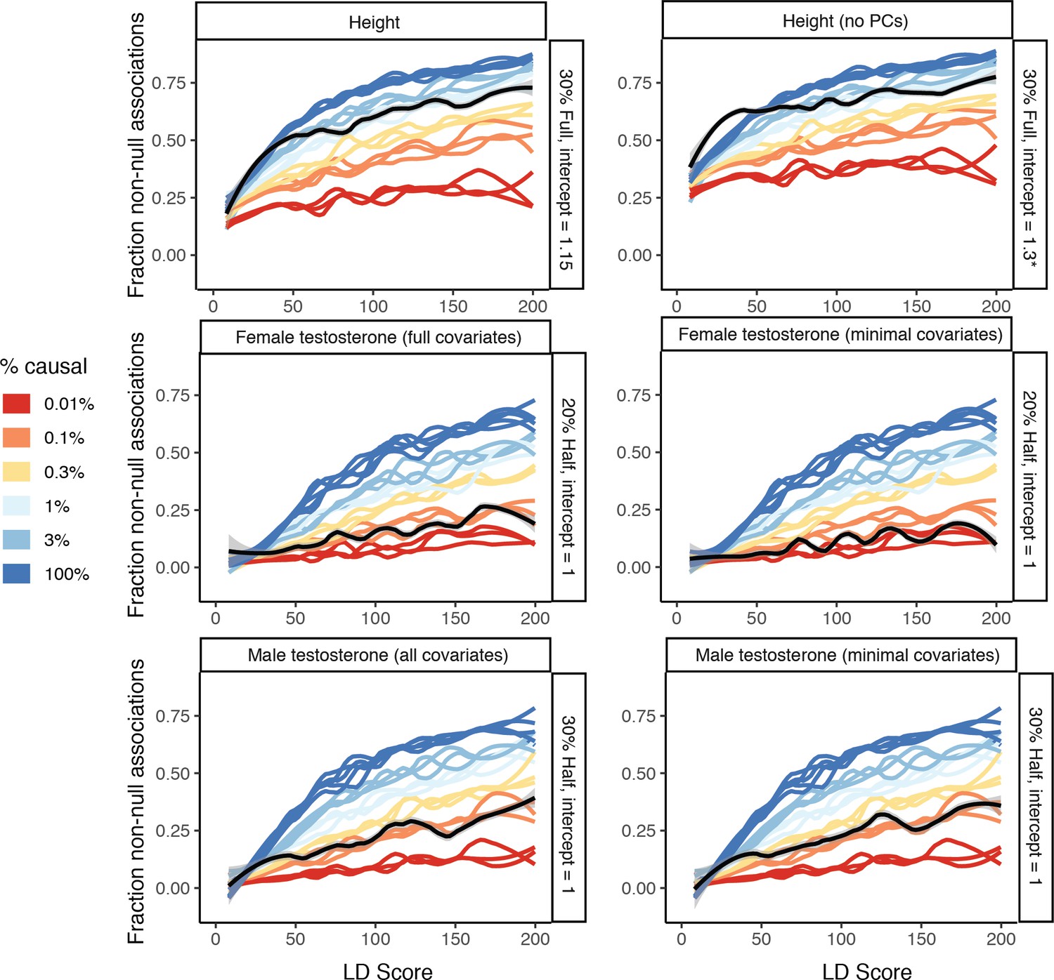
Effect of GWAS covariates on estimates.
As noted in Figure 8—figure supplement 2, not including principal components can meaningfully effect estimates and produce upward bias, so we recommend adjusting for principal components (or using a suitable mixed model). In addition, we evaluated testosterone traits using two covariate sets: the complete set and a minimal age, age2, genotyping array, and principal components 1–20 that were used for the CBAT GWAS (due to the derivation from albumin, SHBG, and testosterone, and the difference in batch between these, Materials and methods). For male testosterone the effect of different covariates was negligible, while for female testosterone, the estimate was slightly lower with the minimal covariates. We recommend optimizing covariates to the sample and traits under study to maximize the interpretability of the causal variant estimation.
Figure 8—figure supplement 13
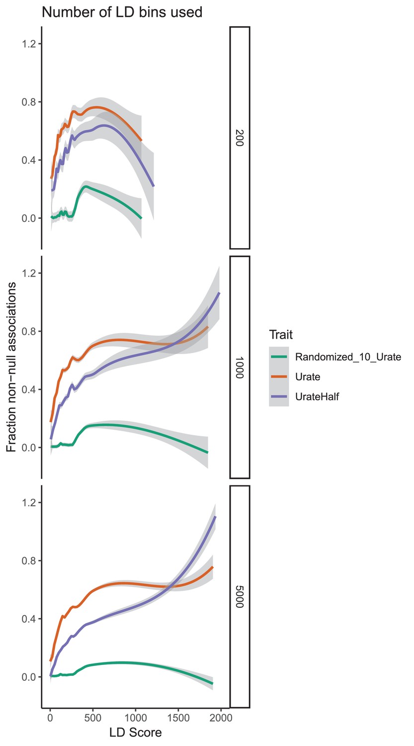
Effect of bin count on estimates of causal variants.
For each binning option, urate, randomized urate, and urate 50% downsampled were run. 1000 bins, 5000 bins, and 200 bins were compared. Lower intercepts and smaller standard errors were observed with higher bin count. We recommend that as many bins as is practicable are used for these analyses.
Figure 8—figure supplement 14
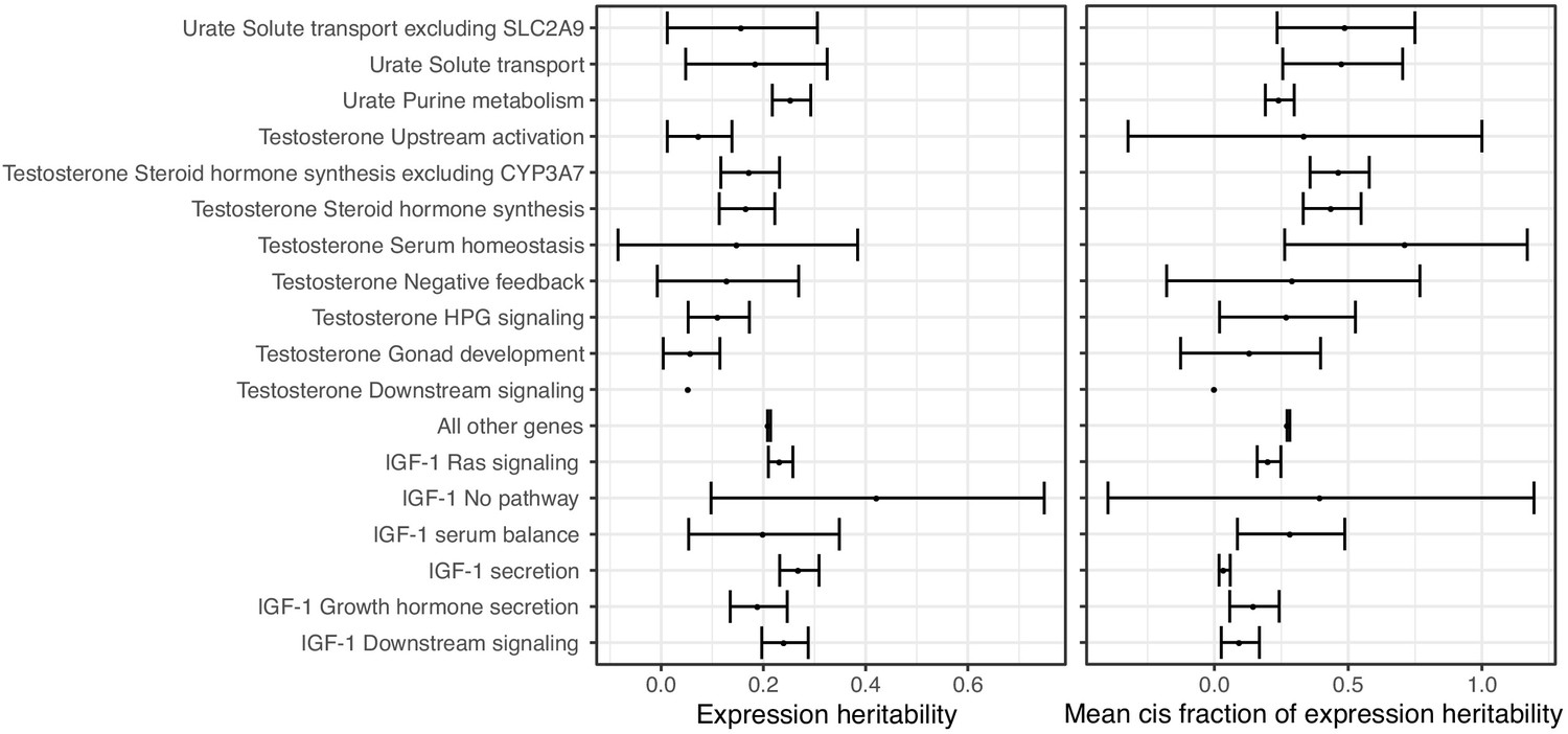
Distributions of (left) total SNP-based heritability of gene expression, or (right) fraction of expression SNP-based heritability driven by cis-effects (Ouwens et al., 2020) for genes in the indicated core pathways, or for all other MsigDB genes not in a core pathway.
Points indicate means, error bars indicate two standard deviations.
Scheme 1
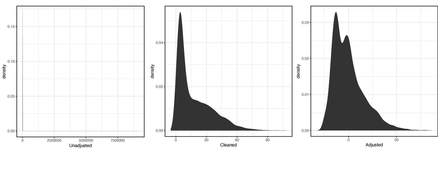
Distribution of raw (left), cleaned (middle), and covariate-adjusted (right) phenotype values for primary luteinizing hormone (LH) code XMOlv.
Scheme 2

Distribution of raw (left), cleaned (middle), and covariate-adjusted (right) phenotype values for secondary LH code XE25I.
Additional files
-
Supplementary file 1
Independent GWAS hits for urate.
CHROM, chromosome number; POS, variant position (hg19); ID, variant identifier; REF, reference genome sequence allele; A1, alternative allele; A1_CT, number of A1 alleles; ALLELE_CT, total alleles; A1_FREQ, frequency of A1 allele; MACH_R2, estimated imputation accuracy (INFO); OBS_CT, number of individuals with non-missing data; BETA, effect size of A1 allele; SE, standard error of A1 allele; T_STAT, t-statistic; P, p-value of association between A1 allele and serum urate levels.
- https://cdn.elifesciences.org/articles/58615/elife-58615-supp1-v1.txt
-
Supplementary file 2
Independent GWAS hits for IGF-1.
CHROM, chromosome number; POS, variant position (hg19); ID, variant identifier; REF, reference genome sequence allele; A1, alternative allele; A1_CT, number of A1 alleles; ALLELE_CT, total alleles; A1_FREQ, frequency of A1 allele; MACH_R2, estimated imputation accuracy (INFO); OBS_CT, number of individuals with non-missing data; BETA, effect size of A1 allele; SE, standard error of A1 allele; T_STAT, t-statistic; P, p-value of association between A1 allele and serum IGF-1 levels.
- https://cdn.elifesciences.org/articles/58615/elife-58615-supp2-v1.txt
-
Supplementary file 3
Independent GWAS hits for testosterone in males.
CHROM, chromosome number; POS, variant position (hg19); ID, variant identifier; REF, reference genome sequence allele; A1, alternative allele; A1_CT, number of A1 alleles; ALLELE_CT, total alleles; A1_FREQ, frequency of A1 allele; MACH_R2, estimated imputation accuracy (INFO); OBS_CT, number of individuals with non-missing data; BETA, effect size of A1 allele; SE, standard error of A1 allele; T_STAT, t-statistic; P, p-value of association between A1 allele and serum testosterone levels in males.
- https://cdn.elifesciences.org/articles/58615/elife-58615-supp3-v1.txt
-
Supplementary file 4
Independent GWAS hits for testosterone in females.
CHROM, chromosome number; POS, variant position (hg19); ID, variant identifier; REF, reference genome sequence allele; A1, alternative allele; A1_CT, number of A1 alleles; ALLELE_CT, total alleles; A1_FREQ, frequency of A1 allele; MACH_R2, estimated imputation accuracy (INFO); OBS_CT, number of individuals with non-missing data; BETA, effect size of A1 allele; SE, standard error of A1 allele; T_STAT, t-statistic; P, p-value of association between A1 allele and serum testosterone levels in females.
- https://cdn.elifesciences.org/articles/58615/elife-58615-supp4-v1.txt
-
Supplementary file 5
Phenotype-level correlations between luteinizing hormone (LH) and testosterone in females and males.
Magnitude of correlation and sample sizes are both higher using the XM0lv luteinizing hormone code, but results are consistent across codes.
- https://cdn.elifesciences.org/articles/58615/elife-58615-supp5-v1.tsv
-
Supplementary file 6
Female-specific association with circulating testosterone levels at the FSHB locus.
We observe an association between the previously discovered rs11031006 (Ruth et al., 2016; Laisk et al., 2018) and serum testosterone levels in females. This association was reproduced in the non-British White individuals in UK Biobank. All effects are at rs11031006 with respect to dosage of the A allele.
- https://cdn.elifesciences.org/articles/58615/elife-58615-supp6-v1.tsv
-
Supplementary file 7
Pathways representing core genes for serum urate biology.
Pathway, which class of genes; Gene name, name of gene included in the given pathway.
- https://cdn.elifesciences.org/articles/58615/elife-58615-supp7-v1.tsv
-
Supplementary file 8
Pathways representing core genes for serum IGF-1 biology.
Pathway, which class of genes; Gene name, name of gene included in the given pathway.
- https://cdn.elifesciences.org/articles/58615/elife-58615-supp8-v1.txt
-
Supplementary file 9
Pathways representing core genes for serum testosterone biology.
Pathway, which class of genes; Gene name, name of gene included in the given pathway.
- https://cdn.elifesciences.org/articles/58615/elife-58615-supp9-v1.txt
-
Supplementary file 10
SNP heritabilities and level of population stratification as estimated by LD Score regression (Finucane et al., 2015) using the full set of baseline and cell-type-specific annotations for each biomarker trait, with height as a baseline.
The lower estimates of LD Score regression SNP-based heritability relative to HESS are expected (Shi et al., 2016). Best intercept refers to the intercept of the inflation for the best-fitting simulation results in the -derived causal SNP estimates (Materials and methods).
- https://cdn.elifesciences.org/articles/58615/elife-58615-supp10-v1.txt
-
Supplementary file 11
Estimates of SNP heritability and fraction of causal variants from GENESIS (Zhang et al., 2018).
K, number of mixture components used in the fit of effect sizes. Half sample, 50% downsample of individuals in GWAS to mimic the sex-specific traits. * Failed to converge and terminated after a single iteration.
- https://cdn.elifesciences.org/articles/58615/elife-58615-supp11-v1.tsv
-
Supplementary file 12
Phenotype-level correlations between luteinizing hormone (LH) and testosterone in females and males.
Magnitude of correlation and sample sizes are both higher using the XM0lv luteinizing hormone code, but results are consistent across codes.
- https://cdn.elifesciences.org/articles/58615/elife-58615-supp12-v1.tsv
-
Transparent reporting form
- https://cdn.elifesciences.org/articles/58615/elife-58615-transrepform-v1.docx
Download links
A two-part list of links to download the article, or parts of the article, in various formats.
Downloads (link to download the article as PDF)
Open citations (links to open the citations from this article in various online reference manager services)
Cite this article (links to download the citations from this article in formats compatible with various reference manager tools)
GWAS of three molecular traits highlights core genes and pathways alongside a highly polygenic background
eLife 10:e58615.
https://doi.org/10.7554/eLife.58615


