Functional reallocation of sensory processing resources caused by long-term neural adaptation to altered optics
- Flaum Eye Institute, University of Rochester Medical Center, United States
- Center for Visual Science, University of Rochester, United States
- Brain and Cognitive Sciences, University of Rochester, United States
- Department of Psychology, University of Washington, United States
- Shanghai Key Laboratory of Psychotic Disorders, Shanghai Mental Health Center, Shanghai Jiao Tong University School of Medicine, China
- Institute of Psychology and Behavioral Science, Shanghai Jiao Tong University, China
- Department of Neuroscience, University of Rochester, United States
Figures
Figure 1
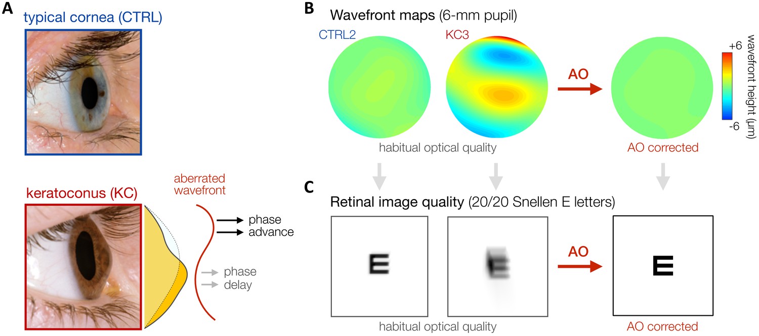
Keratoconus (KC).
(A) KC is a progressive eye disease affecting neurotypically-developed adults, in which the typically round cornea thins and bulges into a cone-like shape. Pictures adapted from http://www.theeyefoundation.com. (B, C) As shown on the wavefront maps , KC results in large amounts of higher-order optical aberrations (HOAs) that cannot be fully corrected using conventional optical devices. As a result, KC patients are chronically exposed to large amounts of habitual optical aberrations and poor retinal image quality in their daily life (simulated for 20/20 Snellen E letter for 6-mm pupil). Adaptive optics (AO) techniques can be used to fully correct all optical aberrations during in-lab visual testing, allowing us to bypass optical factors and directly assess differences in neural visual processing.
Figure 2 with 3 supplements
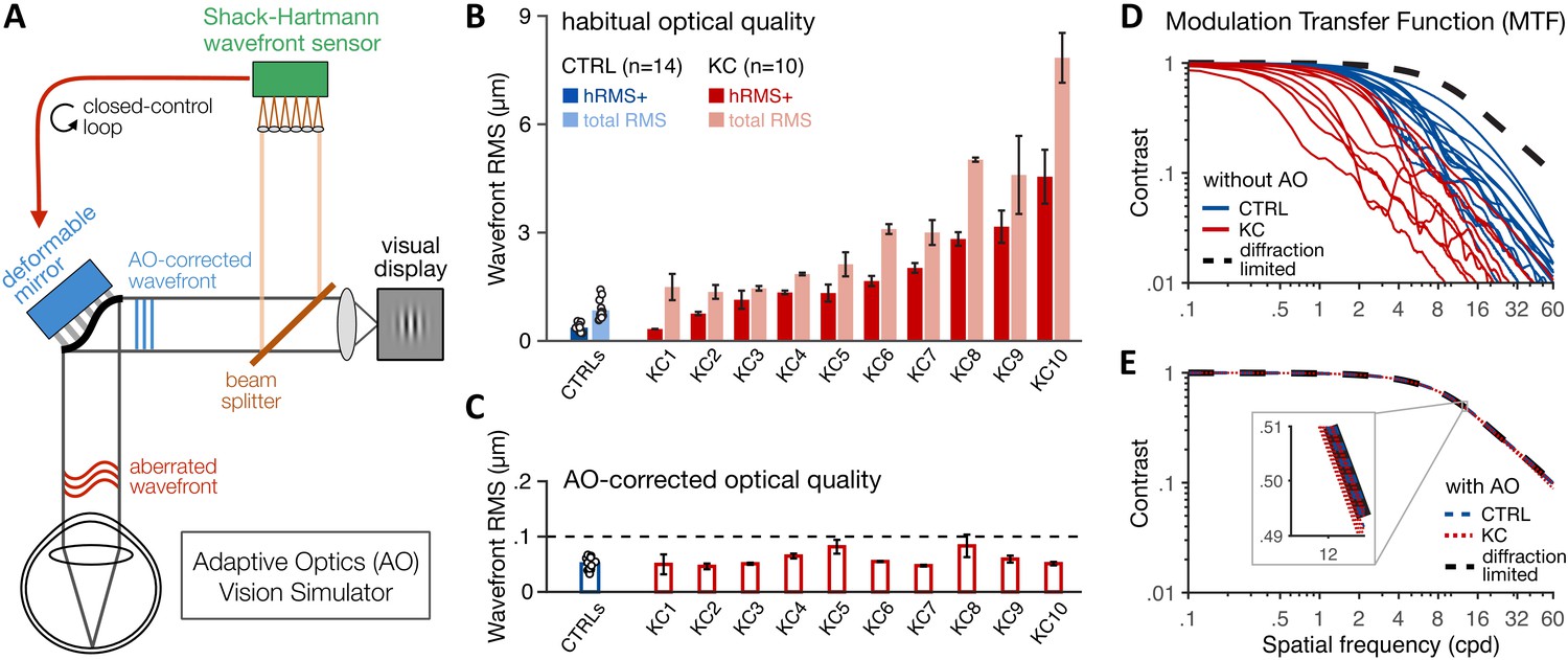
Using adaptive optics (AO) to study long-term exposure to poor optics in keratoconus (KC).
(A) An AO vision simulator was used to maintain aberration-free image quality during visual testing by measuring the subject’s aberrated wavefront using a Shack–Hartmann wavefront sensor and fully correcting it online using a deformable mirror in a closed-control loop. (B) Relative to age-matched control (CTRL) observers with healthy eyes, KC observers were chronically exposed to atypical amounts of habitual optical aberrations (total root mean square [RMS]), with large amounts of higher-order aberrations (hRMS+). Group-average RMS and individual data points are presented for CTRL observers (n = 14). Individual bars for each of the 10 KC patients show the habitual RMS and hRMS+ (±1 SD). (C) AO correction maintained similar, aberration-free optical quality during visual testing, even in severe KC eyes. Note the large difference in y-axis scale between B and C. (D, E) The modulation transfer function (MTF) characterizes how much contrast is transmitted by the eye’s optics as a function of the spatial frequency content of the image. (D) Without AO correction, KC patients (red lines) were subject to severe contrast reductions relative to CTRL observers with healthy eyes (blue lines). (E) Under AO correction, the MTF of both KC and CTRL observers reached similar diffraction-limited optical quality, allowing us to directly measure differences in neural transfer functions between KC and CTRL observers.
Figure 2—figure supplement 1

Description of the adaptive optics vision simulator (AOVS).
(A) Picture of the AOVS used in the Yoon’s lab at the University of Rochester Medical Center. Participants were tested monocularly, while the untested eye was patched. (B) Schematic description of the AOVS. The AOVS allows to measure the aberrated wavefront of the subject’s eye using a Shack–Hartmann wavefront sensor and fully correct it online with a deformable mirror in closed-control loop to ensure aberration-free image quality.
Figure 2—figure supplement 2

Examples of online adaptive optics (AO) correction in control (CTRL) and keratoconus (KC) eyes.
(A) KC10. (B) KC9. (C) CTRL7. Closed-loop AO correction (AO on; blue vertical line) corrected all aberrations and maintained the residual root mean square (RMS) significantly below 0.1 µm during visual testing (red horizontal dashed line). To maximize AO correction during stimulus presentation, participants were trained to blinks between trials and to stop if the perceptual quality got unstable and/or poor quality. Spikes correspond to blinks (indicated by the grey arrows) during which AO correction was paused. The median RMS during AO correction was computed for each measurement to minimize the influence of blinks when estimating the residual RMS under AO correction. To improve AO-correction performance, severe KC eyes were fitted with a scleral lens by one of the ophthalmologists at the University of Rochester Medical Center right before testing. Thus, wavefront patterns before AO correction do not necessarily reflect the habitual optical aberrations experienced by these KC patients in their daily life.
Figure 2—video 1
Online adaptive optics (AO) correction in a severe keratoconus (KC) observer (KC10).
Closed-loop AO correction (AO on; blue vertical line) corrected all optical aberrations and maintained the residual root mean square (RMS) wavefront error significantly below 0.1 µm during visual testing. Same convention as Figure 2—figure supplement 2.
Figure 3
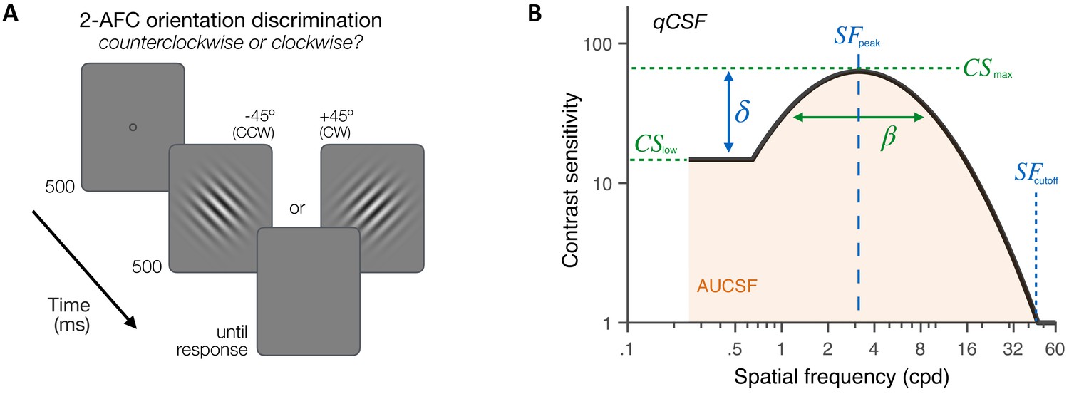
Experiment 1: contrast sensitivity function (CSF) measurement.
(A) Stimuli, task and timeline. Each trial began with a dynamic fixation point. After a blank screen, a ±45°-oriented Gabor stimulus was presented at fixation using a 500-ms temporal Gaussian envelope. Stimuli varied in contrast and spatial frequency (SF) from trial to trial. Observers judged whether the stimulus was tilted ±45° from vertical using a 2 alternative forced choice (AFC) task. Full adaptive optics correction was maintained during testing. (B) Quick CSF method. The qCSF estimates the CSF through four parameters: peak sensitivity (CSmax), peak SF (SFpeak), bandwidth (), and low-SF truncation (δ). The area under the CSF (AUCSF), low-SF sensitivity (CSlow), and high-SF cutoff (SFcutoff) were also estimated from qCSF fits.
Figure 4 with 2 supplements
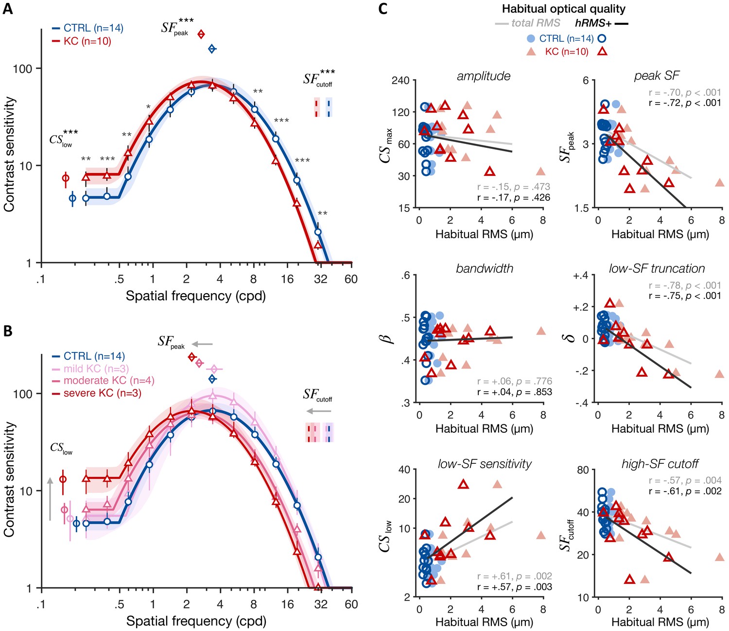
Experiment 1: altered contrast sensitivity function (CSF) following long-term exposure to poor optics.
All results are for visual images fully corrected using adaptive optics (AO), for both keratoconus (KC) and age-matched control (CTRL) observers. (A) qCSF results. Relative to control observers (blue curve), KC patients (red curve) showed altered CSFs that were shifted toward lower SFs, with both impaired high-SF sensitivity and improved low-SF sensitivity. Shaded areas and error bars represent bootstrapped 95% confidence intervals (CIs). Asterisks indicate significant differences computed from bootstrapping between groups (*p<0.05; **p<0.01; ***p<0.001). Comparisons at each of the 12 SFs were corrected for multiple comparisons using Bonferroni correction. (B) Same as A but with KC patients divided into separate groups based on KC severity for illustration purposes (see also Figure 4—figure supplement 1). (C) Link between CSF and habitual optical quality. Altered CSF under AO correction correlated with the amount of habitual optical aberrations of each subject. Each panel shows individual parameter estimates plotted as a function of each subject’s habitual root mean square (RMS; total RMS: light filled symbols; hRMS+: darker open symbols). Linear regression fits and Pearson correlation coefficients are plotted for each RMS measure.
Figure 4—figure supplement 1

Experiment 1: altered contrast sensitivity function (CSF) as a function of KC severity.
qCSF results under full adaptive optics (AO) correction for age-matched control participants (CTRL; blue curve) and keratoconus (KC) patients with (A) mild (N = 3), (B) moderate (N = 4), or (C) severe (N = 3) habitual optical aberrations. Relative to control observers, KC patients showed altered CSF functions that were shifted toward lower spatial frequencies (SFs), with impaired sensitivity at high SFs as well as improved sensitivity at low SFs. This pattern depended on KC severity, with mild KC showing no difference compared to CTRL observers, whereas patients with severe KC showed marked CSF alterations. Shaded areas and error bars represent bootstrapped 95% CIs. Asterisks indicate significant differences computed from bootstrapping between CTRL and KC participants (†p<0.1; *p<0.05; **p<0.01; ***p<0.001). Comparisons at each of the 12 SFs were corrected for multiple comparisons using Bonferroni correction.
Figure 4—figure supplement 2

Experiment 1: altered contrast sensitivity function (CSF) does not depend on participant’s age.
Each panel shows individual CSF parameter estimates plotted as a function of participant’s age (control [CTRL]: blue circles; keratoconus [KC]: red triangles). The pattern of gains and losses we observed at low and high spatial frequencies (SFs), respectively, did not depend on participant's age. Participant's age was associated with a decrease in the area under the CSF (AUCSF) and peak sensitivity (amplitude), consistent with an overall reduction in contrast sensitivity with age. Linear regression fits (solid line) and Pearson correlation coefficients are indicated for each panel.
Figure 5 with 1 supplement
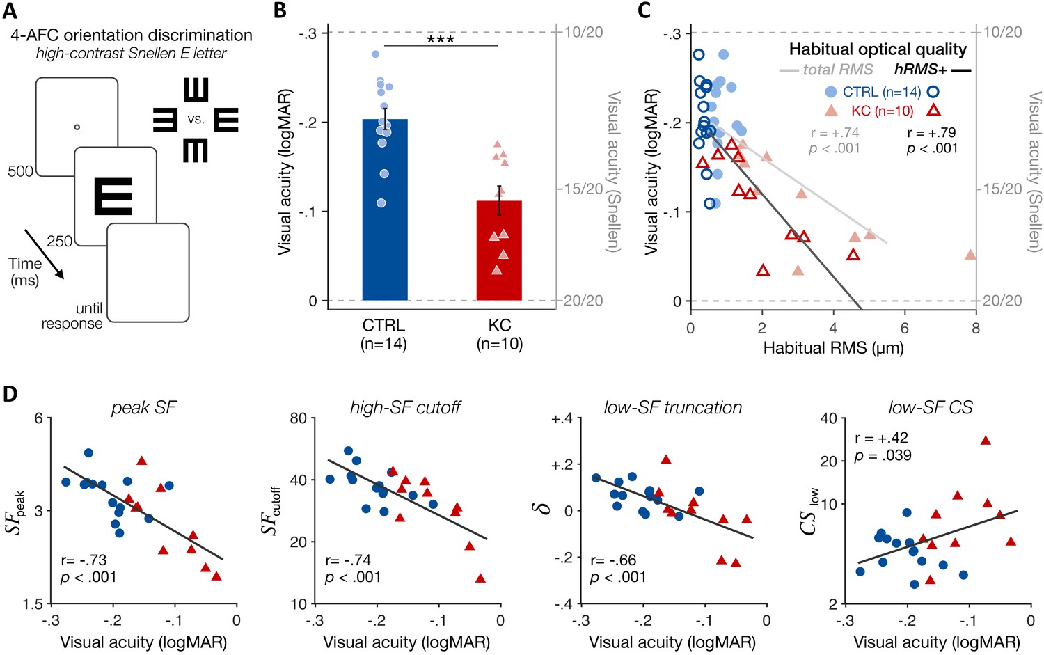
Experiment 2: poorer high-contrast visual acuity (VA) following long-term exposure to poor optics.
(A) VA acuity thresholds were measured under adaptive optics (AO) correction using a four alternative forced choice (AFC) discrimination task. The size of high-contrast, Snellen E letter stimuli varied from trial to trial to estimate 62.5%-correct VA thresholds (in logMAR). (B) Relative to age-matched control (CTRL) observers, keratoconus (KC) patients showed poorer VA despite being tested under similar aberration-free optical conditions. Error bars correspond to ±1 SEM, with each data point representing an individual observer (CTRL: blue circles; KC: red triangles). (C) Poorer habitual optical quality was associated with stronger VA deficits under aberration-free conditions; total root mean square (RMS): all habitual aberrations; hRMS+: higher-order aberrations. (D) Deficits in VA under AO correction correlated with the changes in qCSF parameters observed in experiment 1. Linear regression (solid line) and Pearson correlation coefficients are indicated in C and D.
Figure 5—figure supplement 1

Experiment 2: poorer VA does not depend on participant’s age.
Each panel shows individual VA under adaptive optics correction plotted as a function of participant’s age (control [CTRL]: blue circles; keratoconus [KC]: red triangles). Linear regression fits (solid line) and Pearson correlation coefficients are indicated.
Figure 6
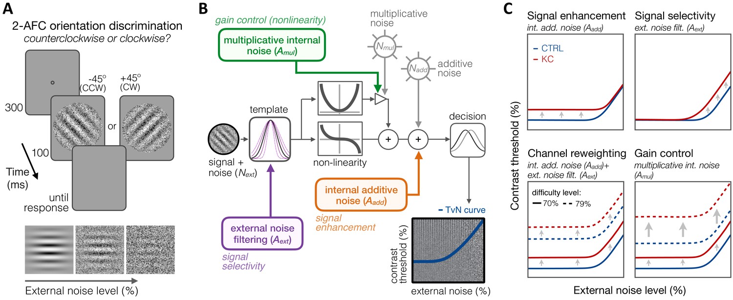
Experiment 3: equivalent noise paradigm and perceptual template model (PTM).
(A) Stimuli, task, and timeline. In each trial, an oriented grating embedded in dynamic Gaussian pixel noise was presented. Observers judged whether stimuli were tilted ±45° from vertical. (B) Schematic representation of the PTM. This model consists of five main components: a perceptual template processing signals embedded in external noise (Next), a nonlinear transducer function, two internal noise sources (multiplicative Nmul and additive Nadd), and a decision process. The output of the decision process models limitations in sensitivity as equivalent internal noise, with threshold-vs-noise (TvN) curves having a characteristic nonlinear shape. At low external noise, internal noise dominates and added external noise has little effect, resulting in the TvN curve’s flat segment. Once external noise level exceeds that of internal noise, stronger signal contrast is needed to overcome added external noise, resulting in the TvN curve’s rising segment. Adapted from Lu and Dosher, 2008. (C) Predictions. Distinct mechanisms can account for group differences between control (CTRL) and keratoconus (KC) participants. (1, upper left) Elevated internal additive noise (Aadd) yields increased thresholds at the TvN curve’s flat portion, reflecting differences in signal enhancement mechanisms.(2, upper right) Poorer external noise filtering (Aext) limits thresholds at the TvN curve’s rising portion, reflecting differences in signal selectivity (tuning). (3, lower left) A combination of the two results in increased thresholds across external noise levels and difficulty levels, and suggests channel reweighting. (4, lower right) Elevated multiplicative internal noise (Amul) results in a similar pattern across external levels but the differences scale with difficulty levels (i.e., signal contrast), acting similarly to a gain control mechanism (nonlinearity change).
Figure 7 with 7 supplements
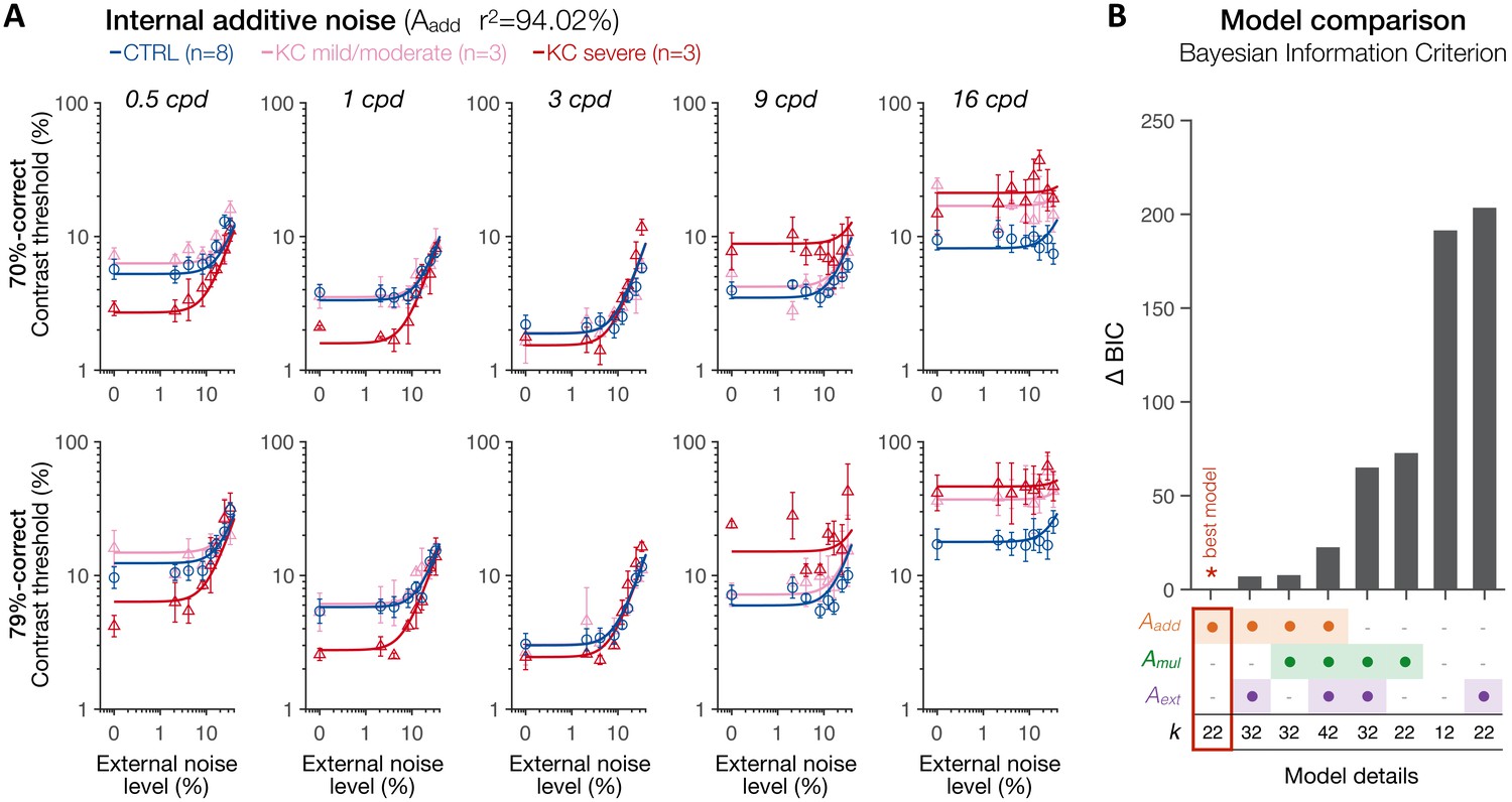
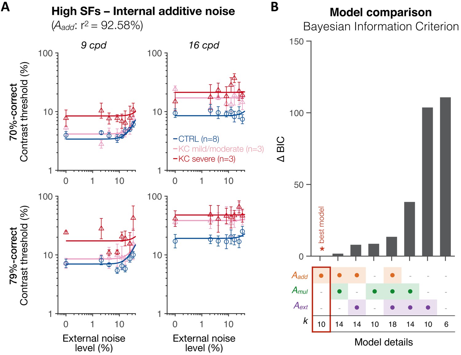
Experiment 3: spatial frequency (SF) specific changes in internal additive noise mediate contrast sensitivity differences following long-term exposure to optical defects.
(A) Contrast thresholds were measured under full adaptive optics (AO) correction as a function of external noise levels for five different SFs (0.5, 1, 3, 9, and 16 cpd) and for 70.71%-correct (upper row) and 79.37%-correct (lower row) difficulty levels. Relative to control (CTRL) observers, severe keratoconus (KC) patients showed impaired thresholds at high SFs and better thresholds at low SFs. These group differences were observed at low, but not at high, external noise levels, and were less pronounced in KC patients with mild-to-moderate amounts of habitual optical aberrations. Data were fitted with the perceptual template model to evaluate the contribution of distinct sources of inefficiencies: internal additive noise (Aadd), multiplicative internal noise (Amul), external noise filtering (Aext), or any combination of these factors. The best model explaining the differences between groups was the internal additive noise model. (B) Model comparisons. Bayesian information criterion (BIC) evidence was computed for each model to identify which model best explained the data while penalizing for a greater number of free parameters (k). The value of the best model was subtracted from all BIC values (∆BIC). The best model (∆BIC = 0) was the model assuming solely changes in internal additive noise across SFs between CTRL and KC groups.
Figure 7—figure supplement 1

Experiment 3: results of the full model and of the internal additive noise model.
(A) Full model. (B) Internal additive noise model. Each symbol represents the average contrast thresholds for each group ±1 SEM error bars, with the solid lines representing the fits of the perceptual template model. Aadd: internal additive noise; Amul: multiplicative internal noise; Aext: external noise filtering; CTRL: control; KC: keratoconus.
Figure 7—figure supplement 2
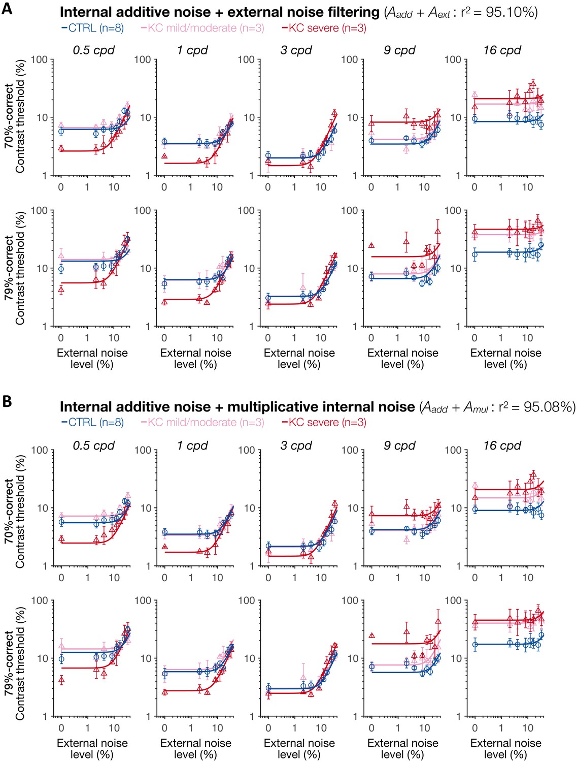
Experiment 3: results of the two mixture models with internal additive noise.
(A) Internal additive noise + external noise filtering model. (B) Internal additive noise + multiplicative internal noise model. Each symbol represents the average contrast thresholds for each group ±1 SEM error bars, with the solid lines representing the fits of the perceptual template model. Aadd: internal additive noise; Amul: multiplicative internal noise; Aext: external noise filtering; CTRL: control; KC: keratoconus.
Figure 7—figure supplement 3
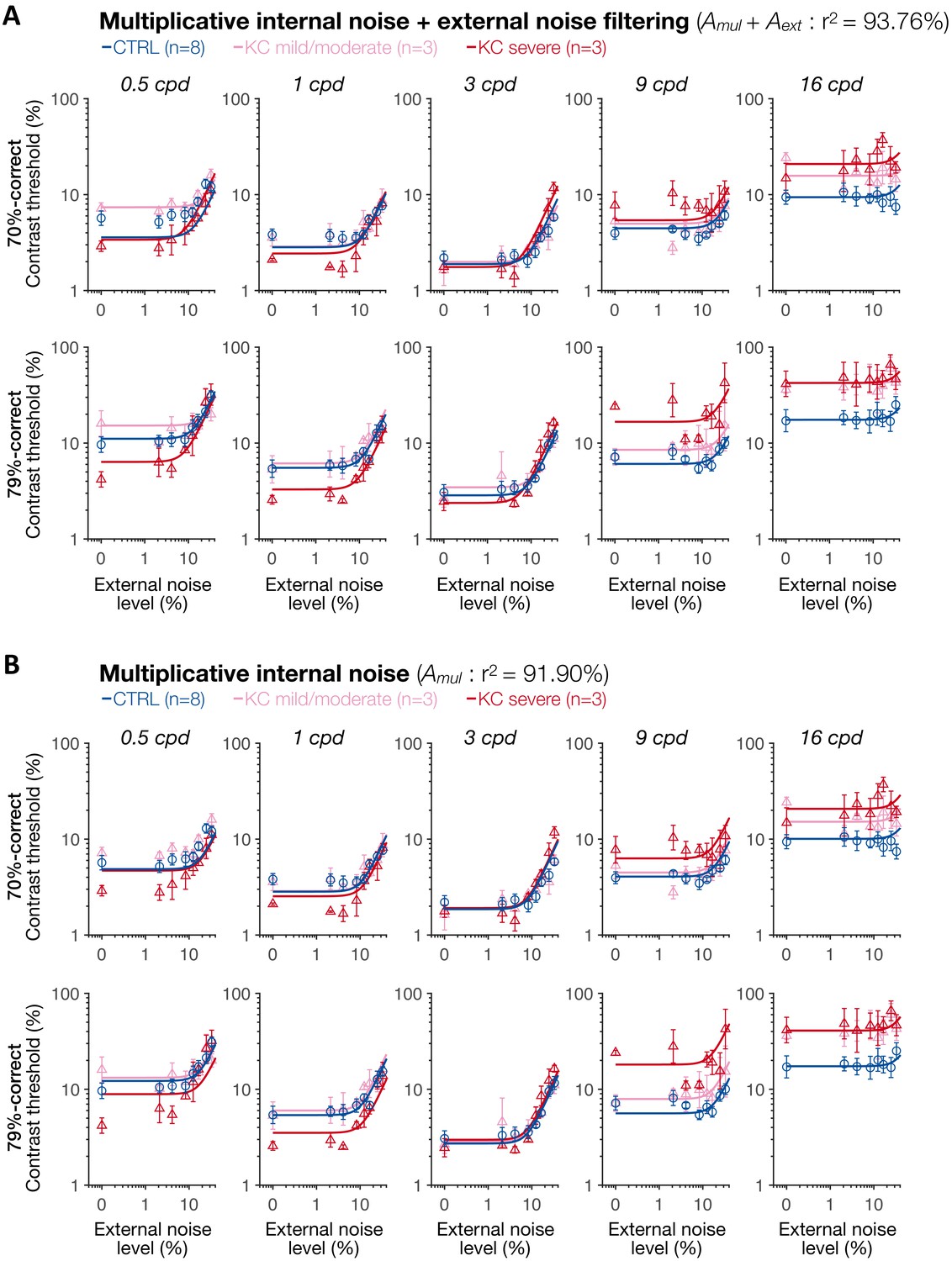
Experiment 3: results of the multiplicative internal noise + external noise filtering model and multiplicative internal noise model.
(A) Multiplicative internal noise + external noise filtering model. (B) Multiplicative internal noise model. Each symbol represents the average contrast thresholds for each group ±1 SEM error bars, with the solid lines representing the fits of the perceptual template model. Aadd: internal additive noise; Amul: multiplicative internal noise; Aext: external noise filtering; CTRL: control; KC: keratoconus.
Figure 7—figure supplement 4

Experiment 3: results of the external noise filtering model and of the null model.
(A) External noise filtering model. (B) Null model. Each symbol represents the average contrast thresholds for each group ± 1 SEM error bars, with the solid lines representing the fits of the perceptual template model. Aadd: internal additive noise; Amul: multiplicative internal noise; Aext: external noise filtering; CTRL: control; KC: keratoconus.
Figure 7—figure supplement 5

Experiment 3: independent analysis for low spatial frequencies (SFs) supports the internal additive noise model.
(A) At low SFs, the differences in contrast thresholds between control (CTRL) and keratoconus (KC) observers were best explained by changes only in internal additive noise (Aadd), reflecting improved signal enhancement in patients with severe KC. (B) Bayesian information criterion (BIC) evidence was computed for each model, and the value from the best model was subtracted. The best model (∆BIC = 0) was a model assuming changes only in internal additive noise between control and KC observers, consistent with the results across SFs. Aadd: internal additive noise; Amul: multiplicative internal noise; Aext: external noise filtering; k: number of free parameters.
Figure 7—figure supplement 6
Experiment 3: independent analysis for high spatial frequencies (SFs) supports the internal additive noise model.
(A) At high SFs, the differences in contrast thresholds between control (CTRL) and keratoconus (KC) observers were best explained by changes only in internal additive noise (Aadd), reflecting impaired signal enhancement in patients with severe KC. (B) Bayesian information criterion (BIC) evidence was computed for each model, and the value from the best model was subtracted. The best model (∆BIC = 0) was a model assuming changes only in internal additive noise between control and KC observers, consistent with the results across SFs. Aadd: internal additive noise; Amul: multiplicative internal noise; Aext: external noise filtering; k: number of free parameters.
Figure 7—figure supplement 7
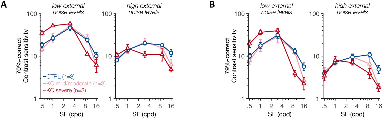
Experiment 3: contrast sensitivity function at low and high external noise levels.
(A, B) Contrast sensitivity (1/threshold) was computed as a function of the stimulus spatial frequency (SF) using either the two lowest external noise values (left panels) or the two highest external noise values (right panels), at (A) 70.71%-correct and (B) 79.37%- correct levels of difficulty. Each symbol represents average values ± 1 SEM error bars for each group. A similar pattern was observed across difficulty levels. At low external noise, SF-specific differences in contrast sensitivity were observed between control (CTRL) participants and severe keratoconus (KC) patients, replicating the alterations in qCSF found in experiment 1.
Figure 8
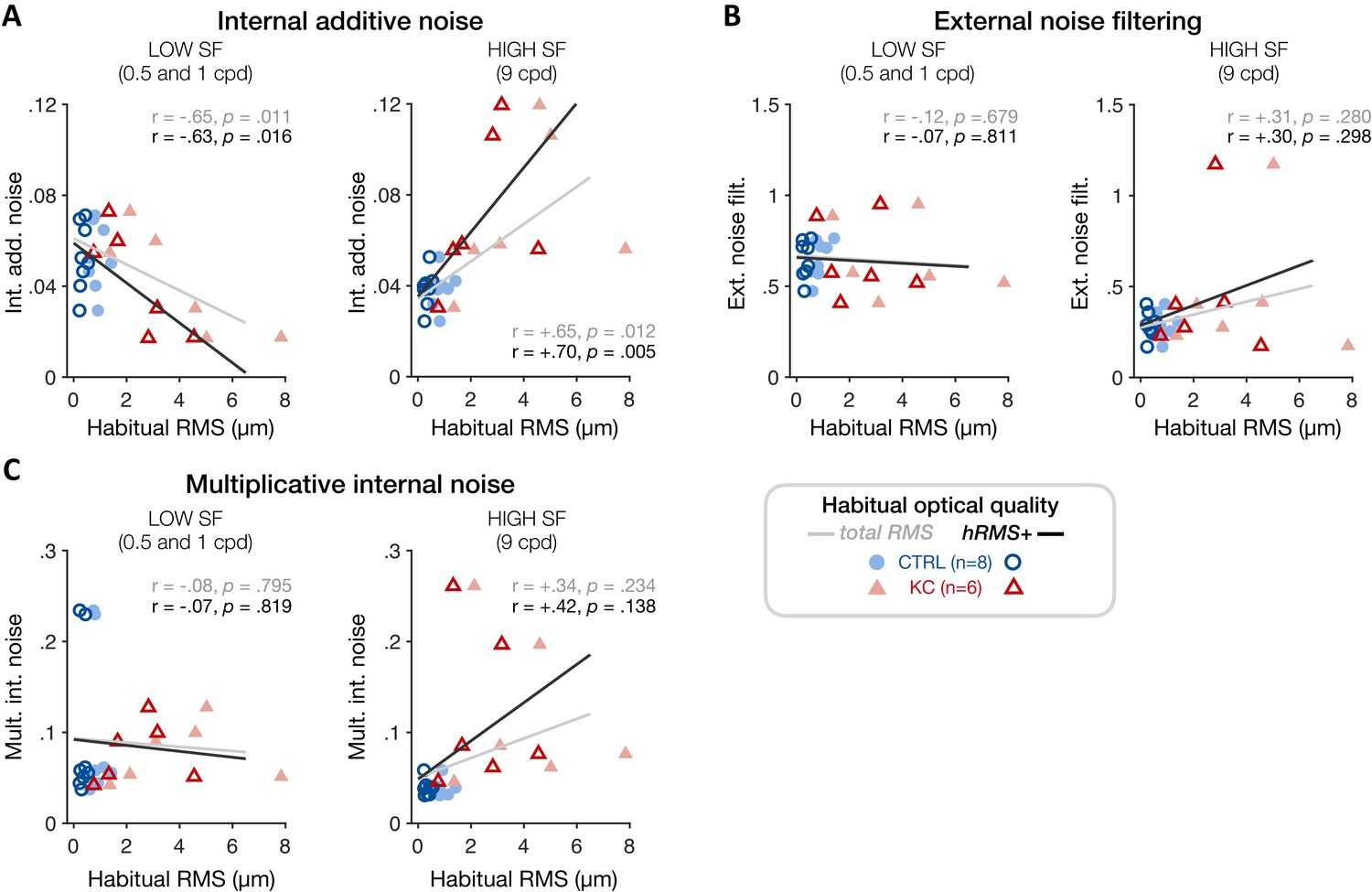
Experiment 3: correlation between individual noise estimates and participants’ habitual optical quality at low and high spatial frequencies (SFs).
(A) Poorer habitual optical quality was associated with SF-specific changes in internal additive noise, with reduced internal additive noise at low SFs (left panel) and elevated internal additive noise at high SFs (right panel). Other noise estimates (B: external noise filtering; C: multiplicative internal noise) did not correlate with habitual optical quality, consistent with internal additive noise being the primary source of inefficiency mediating the effects of long-term exposure to poor optical quality. Data points correspond to individual estimates (CTRL: control, blue circles; KC: keratoconus, red triangles) plotted as a function of the participant’s habitual root mean square (RMS) wavefront error (i.e., total RMS: all habitual aberrations; hRMS+: higher-order aberrations).
Tables
Table 1
Participant information.
| Participant | Gender | Age (years) | Total RMS (µm) | hRMS+ (µm) | AO RMS (µm) | Experiments | Habitual optical aberrations | |
|---|---|---|---|---|---|---|---|---|
| Tested eye | Untested eye | |||||||
| KC1 | F | 40 | 1.49 | 0.33 | 0.050 | qCSF | VA | Mild | Mild |
| KC2 | F | 24 | 1.36 | 0.76 | 0.046 | qCSF | VA | PTM | Mild | Moderate |
| KC3 | M | 27 | 1.46 | 1.14 | 0.051 | qCSF | VA | Mild | Mild |
| KC4 | M | 43 | 1.85 | 1.34 | 0.065 | qCSF | VA | Moderate | Moderate |
| KC5 | M | 27 | 2.12 | 1.33 | 0.082 | qCSF | VA | PTM | Moderate | Moderate |
| KC6 | M | 27 | 3.10 | 1.66 | 0.055 | qCSF | VA | PTM | Moderate | Mild |
| KC7 | F | 22 | 3.00 | 2.02 | 0.047 | qCSF | VA | Moderate | Moderate |
| KC8 | M | 28 | 5.02 | 2.82 | 0.083 | qCSF | VA | PTM | Severe | Moderate |
| KC9 | M | 54 | 4.60 | 3.16 | 0.059 | qCSF | VA | PTM | Severe | Mild |
| KC10 | M | 55 | 7.84 | 4.55 | 0.051 | qCSF | VA | PTM | Severe | Mild |
| KCs (n = 10) | 3 F | 7 M | 34.7 ± 12.4 | 3.18 ± 2.09 | 1.91 ± 1.27 | 0.059 ±0. 014 | |||
| CTRLs (n = 14) | 3 F | 11 M | 33.6 ± 12.3 | 0.84 ± 0.26 | 0.37 ± 0.11 | 0.051 ±0. 011 | |||
| KCs: patients with keratoconus; CTRLs: controls with healthy eyes; M: male; F: female; RMS: root mean square wavefront error computed for a 6-mm pupil size; total RMS: all habitual optical aberrations; hRMS+: higher-order aberrations; AO RMS: residual RMS under adaptive optics (AO) correction; qCSF: quick contrast sensitivity function (experiment 1); VA: visual acuity (experiment 2); PTM: perceptual template model (experiment 3). | ||||||||
Additional files
Download links
A two-part list of links to download the article, or parts of the article, in various formats.
Downloads (link to download the article as PDF)
Open citations (links to open the citations from this article in various online reference manager services)
Cite this article (links to download the citations from this article in formats compatible with various reference manager tools)
Functional reallocation of sensory processing resources caused by long-term neural adaptation to altered optics
eLife 10:e58734.
https://doi.org/10.7554/eLife.58734


