Tracking prototype and exemplar representations in the brain across learning
- Department of Psychology, University of Oregon, United States
- Department of Psychology, University of Wisconsin-Milwaukee, United States
Figures
Figure 1
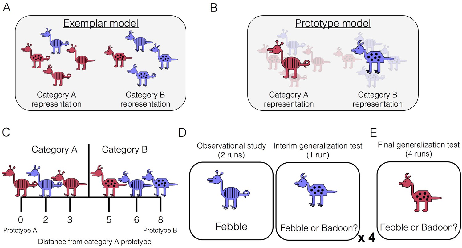
Category-learning task.
Conceptual depiction of (A) exemplar and (B) prototype models. Exemplar: categories are represented as individual exemplars. New items are classified into the category with the most similar exemplars. Prototype: categories are represented by their central tendencies (prototypes). New items are classified into the category with the most similar prototype. (C) Example stimuli. The leftmost stimulus is the prototype of category A and the rightmost stimulus is the prototype of category B, which shares no features with prototype A. Members of category A share more features with prototype A than prototype B, and vice versa. (D) During the learning phase, participants completed four study-test cycles while undergoing fMRI. In each cycle, there were two runs of observational study followed by one run of an interim generalization test. During observational study runs, participants saw training examples with their species labels without making any responses. During interim test runs, participants classified training items as well as new items at varying distances. (E) After all study-test cycles were complete, participants completed a final generalization test that was divided across four runs. Participants classified training items as well as new items at varying distances.
Figure 2

Regions of interest from a representative subject.
Regions were defined in the native space of each subject using automated segmentation in Freesurfer.
Figure 3
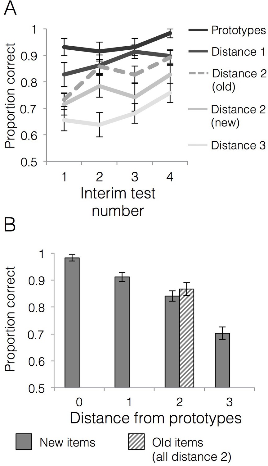
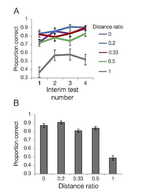
Behavioral accuracy for interim and final tests.
(A) Mean generalization accuracy across each of four interim tests completed during the learning phase. Source data can be found in Figure 3—source data 1. (B) Mean categorization accuracy in the final test. Source data can be found in Figure 3—source data 2. In both cases, accuracies are separated by distance from category prototypes (0–3) and old vs. new (applicable to distance two items only). Error bars represent the standard error of the mean.
-
Figure 3—source data 1
Behavioral accuracy - interim tests.
- https://cdn.elifesciences.org/articles/59360/elife-59360-fig3-data1-v2.csv.zip
-
Figure 3—source data 2
Behavioral accuracy - final test.
- https://cdn.elifesciences.org/articles/59360/elife-59360-fig3-data2-v2.csv.zip
Figure 4
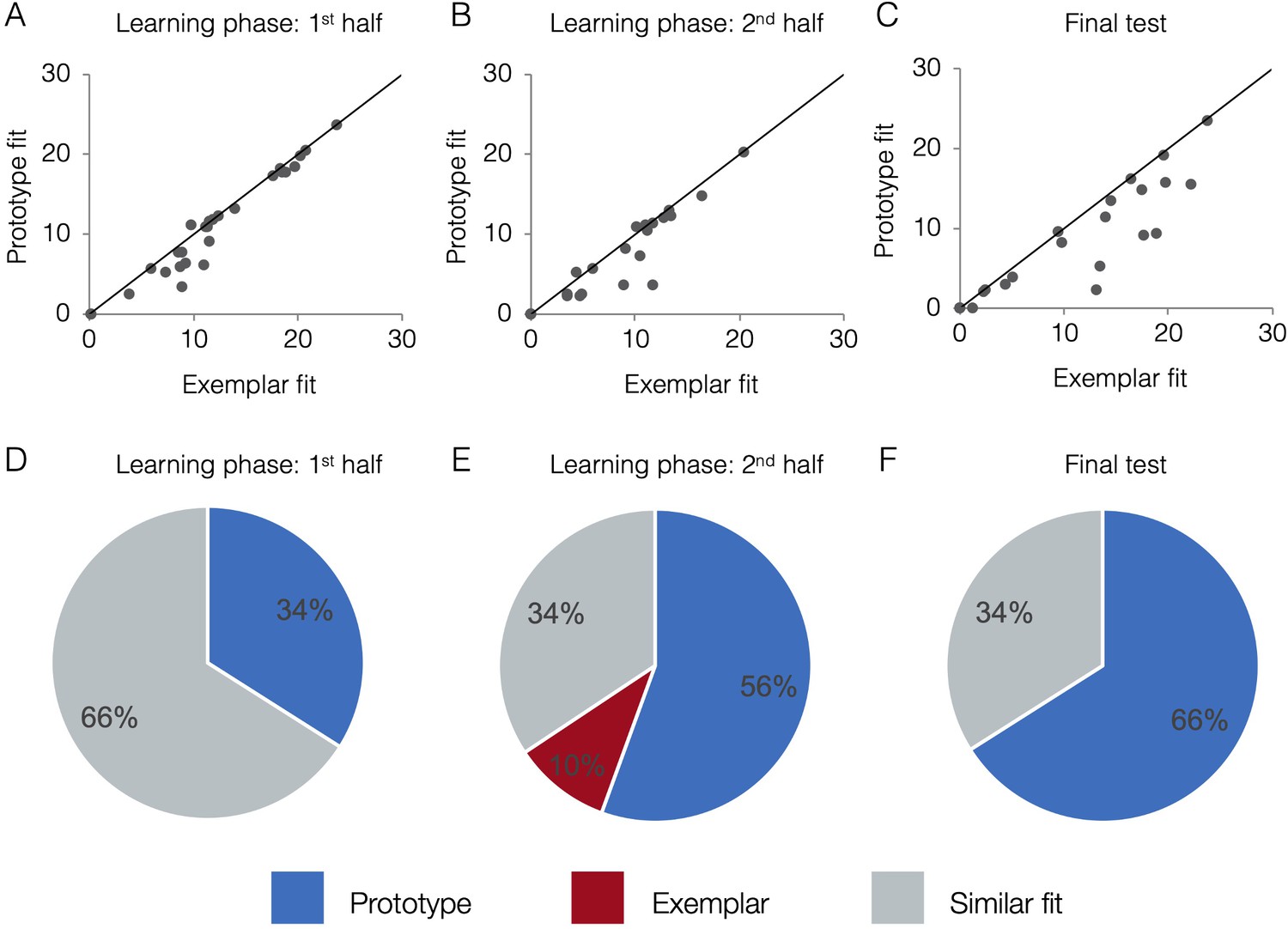
Behavioral model fits.
Scatter plots indicate the relative exemplar vs. prototype model fits for each subject. Fits are given in terms of negative log likelihood (i.e., model error) such that lower values reflect better model fit. Each dot represents a single subject and the trendline represents equal prototype and exemplar fit. Dots above the line have better exemplar relative to prototype model fit. Dots below the line have better prototype relative to exemplar model fit. Pie charts indicate the percentage of individual subjects classified as best fit by the prototype model (in blue), the exemplar model (in red), and those similarly fit by the two models (in grey). Model fits were computed separately for the 1st half of the learning phase (interim tests 1–2, A,D), the 2nd half of the learning phase (interim tests 3–4, B,E), and the final test (C,F). Source data for all phases can be found in Figure 4—source data 1.
-
Figure 4—source data 1
Behavioral model fits - all phases.
- https://cdn.elifesciences.org/articles/59360/elife-59360-fig4-data1-v2.csv.zip
Figure 5
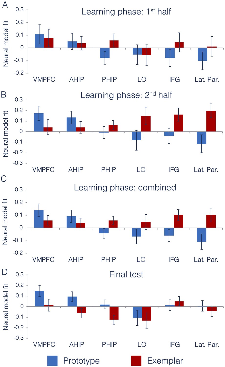
Neural prototype and exemplar model fits.
Neural model fits for each region of interest for (A) the first half of the learning phase, (B) the second half of the learning phase, (C) the overall learning phase (averaged across the first and second half of learning), and (D) the final test. Prototype fits are in blue, exemplar fits in red. Neural model fit is the effect size: the mean/SD of ß-values within each ROI, averaged across appropriate runs. VMPFC = ventromedial prefrontal cortex, ahip = anterior hippocampus, phip = posterior hippocampus, LO = lateral occipital cortex, IFG = inferior frontal gyrus, and Lat. Par. = lateral parietal cortex. Source data for interim tests is in Figure 5—source data 1 and Figure 5—source data 2 for the final test.
-
Figure 5—source data 1
Neural model fits - interim tests.
- https://cdn.elifesciences.org/articles/59360/elife-59360-fig5-data1-v2.csv.zip
-
Figure 5—source data 2
Neural model fits - final test.
- https://cdn.elifesciences.org/articles/59360/elife-59360-fig5-data2-v2.csv.zip
Author response image 1
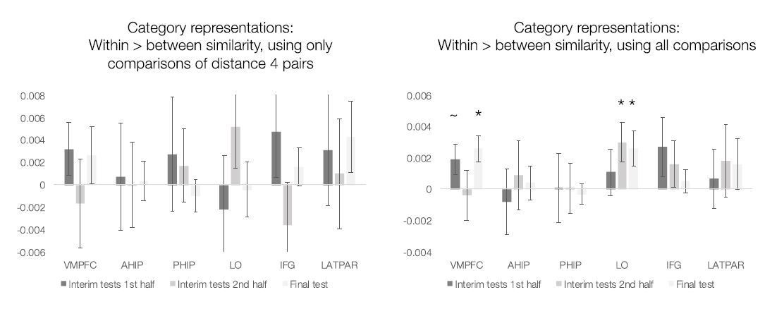
Author response image 2

Author response image 3

Author response image 4

Author response image 5
Tables
Table 1
ANOVA results for model-based fMRI during the learning phase.
| Effect | df | F | P | |
|---|---|---|---|---|
| ROI | 3.4,95.6 GG | 3.90 | .002 | .12 |
| Model | 1,28 | 2.60 | .12 | .09 |
| Learning half | 1,28 | 2.18 | .15 | .07 |
| ROI x Model | 2.9,80.3 GG | 5.91 | .001 | .17 |
| ROI x Learning half | 3.1,86.9 GG | 0.53 | .67 | .02 |
| Model x Learning half | 1,28 | 0.09 | .76 | .003 |
| ROI x Model x Learning Half | 3.2,89.6 GG | 2.31 | .08 | .08 |
Table 2
Dimension values for example prototypes and training stimuli from each category.
| Dimension values | ||||||||
|---|---|---|---|---|---|---|---|---|
| Stimulus | 1 | 2 | 3 | 4 | 5 | 6 | 7 | 8 |
| Prototype A | 1 | 1 | 1 | 1 | 1 | 1 | 1 | 1 |
| A1 | 1 | 1 | 1 | 1 | 1 | 1 | 0 | 0 |
| A2 | 0 | 1 | 1 | 1 | 0 | 1 | 1 | 1 |
| A3 | 1 | 0 | 1 | 0 | 1 | 1 | 1 | 1 |
| A4 | 1 | 1 | 0 | 1 | 1 | 0 | 1 | 1 |
| Prototype B | 0 | 0 | 0 | 0 | 0 | 0 | 0 | 0 |
| B1 | 0 | 0 | 0 | 0 | 0 | 0 | 1 | 1 |
| B2 | 1 | 0 | 0 | 0 | 1 | 0 | 0 | 0 |
| B3 | 0 | 1 | 0 | 1 | 0 | 0 | 0 | 0 |
| B4 | 0 | 0 | 1 | 0 | 0 | 1 | 0 | 0 |
Author response table 1
| Phase | Model | Feature weights (w) | Sensitivity (C) | |||||||
|---|---|---|---|---|---|---|---|---|---|---|
| Neck | Tail | Feet | Nose | Ears | Color | Body | Pattern | |||
| Immediate tests 1-2 | Exemplar | .12 | .15 | .16 | .18 | .10 | .11 | .10 | .08 | 36.6 |
| Prototype | .13 | .13 | .15 | .17 | .09 | .12 | .10 | .09 | 24.7 | |
| Immediate tests 3-4 | Exemplar | .09 | .15 | .15 | .11 | .15 | .08 | .14 | .13 | 56.1 |
| Prototype | .10 | .15 | .16 | .11 | .12 | .10 | .14 | .13 | 49.3 | |
| Final test | Exemplar | .11 | .16 | .14 | .15 | .13 | .06 | .14 | .12 | 57.9 |
| Prototype | .11 | .15 | .16 | .13 | .11 | .09 | .17 | .09 | 49.7 |
Additional files
Download links
A two-part list of links to download the article, or parts of the article, in various formats.
Downloads (link to download the article as PDF)
Open citations (links to open the citations from this article in various online reference manager services)
Cite this article (links to download the citations from this article in formats compatible with various reference manager tools)
Tracking prototype and exemplar representations in the brain across learning
eLife 9:e59360.
https://doi.org/10.7554/eLife.59360


