Entorhinal-retrosplenial circuits for allocentric-egocentric transformation of boundary coding
- Max Planck Institute for Brain Research, Germany
- Institute of Neurophysiology, Neuroscience Center, Goethe University, Germany
Figures
Figure 1 with 4 supplements
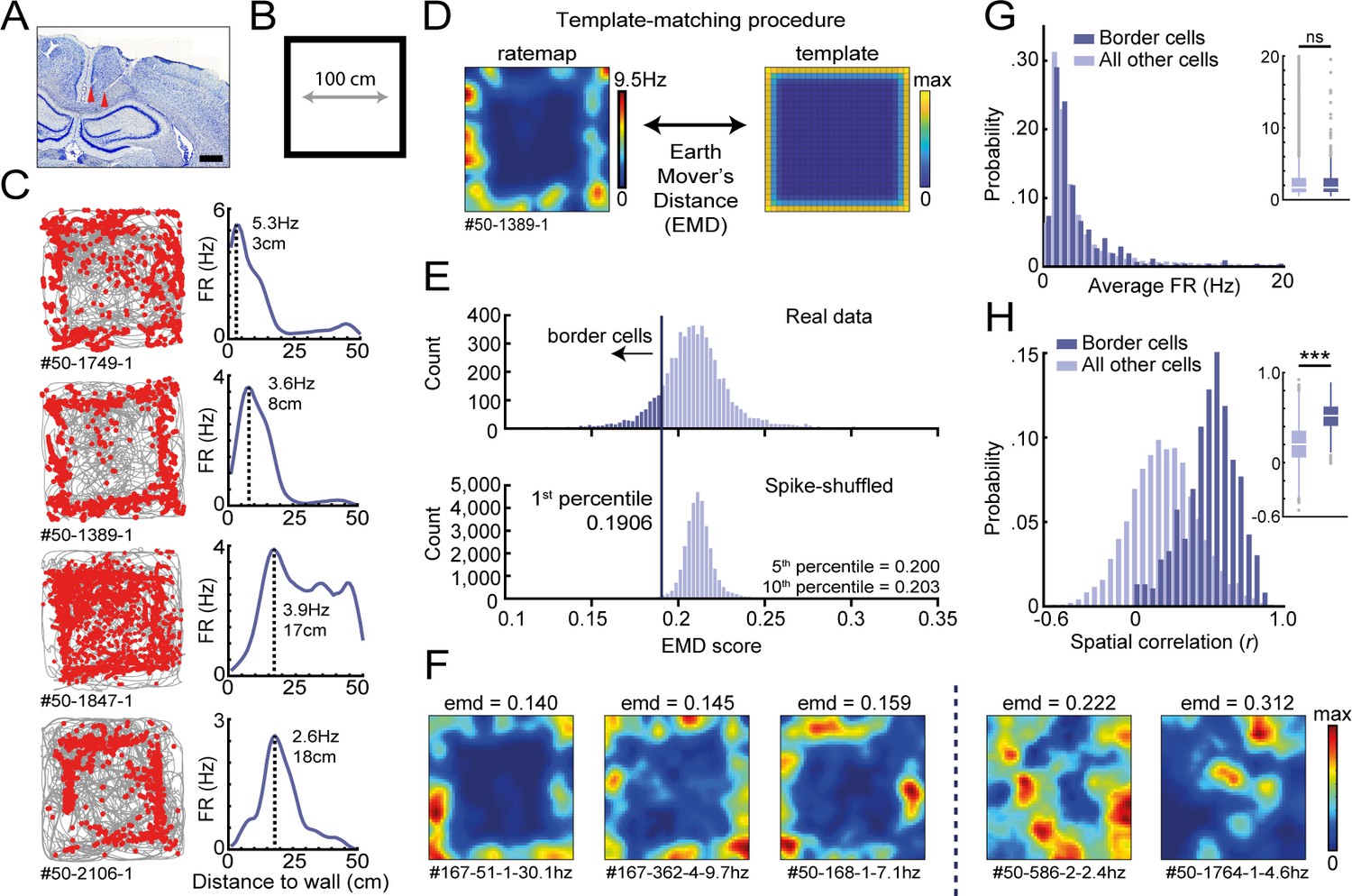
Response profiles of border cells in RSC.
(A) Location of tetrode tracts marked with red in an example Nissl-stained coronal section. Scale bar, 1000 μm. (B) Task behavior consisted of free exploration in a squared 1 m2 arena. (C) Trajectory spike plots (left column) and distance firing rate (FR) plots (right column) of four example cells that fired at different distances away from the wall, relative to the closest wall at any time. Gray lines indicate the animal's trajectory and red dots the rat's position when a spike occurred. (D) A template-matching procedure was applied to classify border cells by calculating the Earth Mover's Distance (EMD) between each cell's spatial rate map and an ideal template (see Materials and methods). (E) A cell was classified as a border cell when its EMD score was below the 1st percentile of a shuffled null distribution, together with an average FR above 0.5 Hz. (F) Color-coded spatial rate maps of five example cells with different EMD scores, where warm colors indicate high firing. From left to right: three typical border cells, a non-uniform firing cell, and a cell with focused firing fields. (G) Distribution of average FR over the entire recording day shows no difference between border cells and other recorded cells. (H) Distribution of spatial correlations between recorded sessions shows significantly higher spatial correlations for border cells compared to other recorded cells. ***p<0.001, Wilcoxon ranksum test.
Figure 1—figure supplement 1
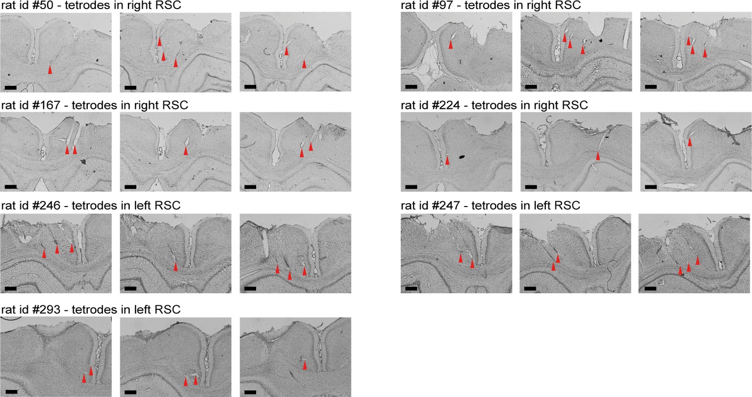
Nissl-stained coronal sections showing recording locations and tetrode tracts for all recording experiments.
Shown are three coronal sections for each of the seven animals included in the electrophysiological experiments. The top two rows include four rats (rats #50, #97, #167, and #224) with the electrode implanted in the right hemisphere, and the bottom rows show sections of three rats with a drive in the left hemisphere (rats #246, #247, and #293). Recordings started at approximately 1 mm below the surface of the cortex and continued in a medioventral direction with a 25° angle until tetrodes reached either the midline or corpus callosum. Red triangles indicate the end of tetrode tracts. Scale bars, 500 μm.
Figure 1—figure supplement 2
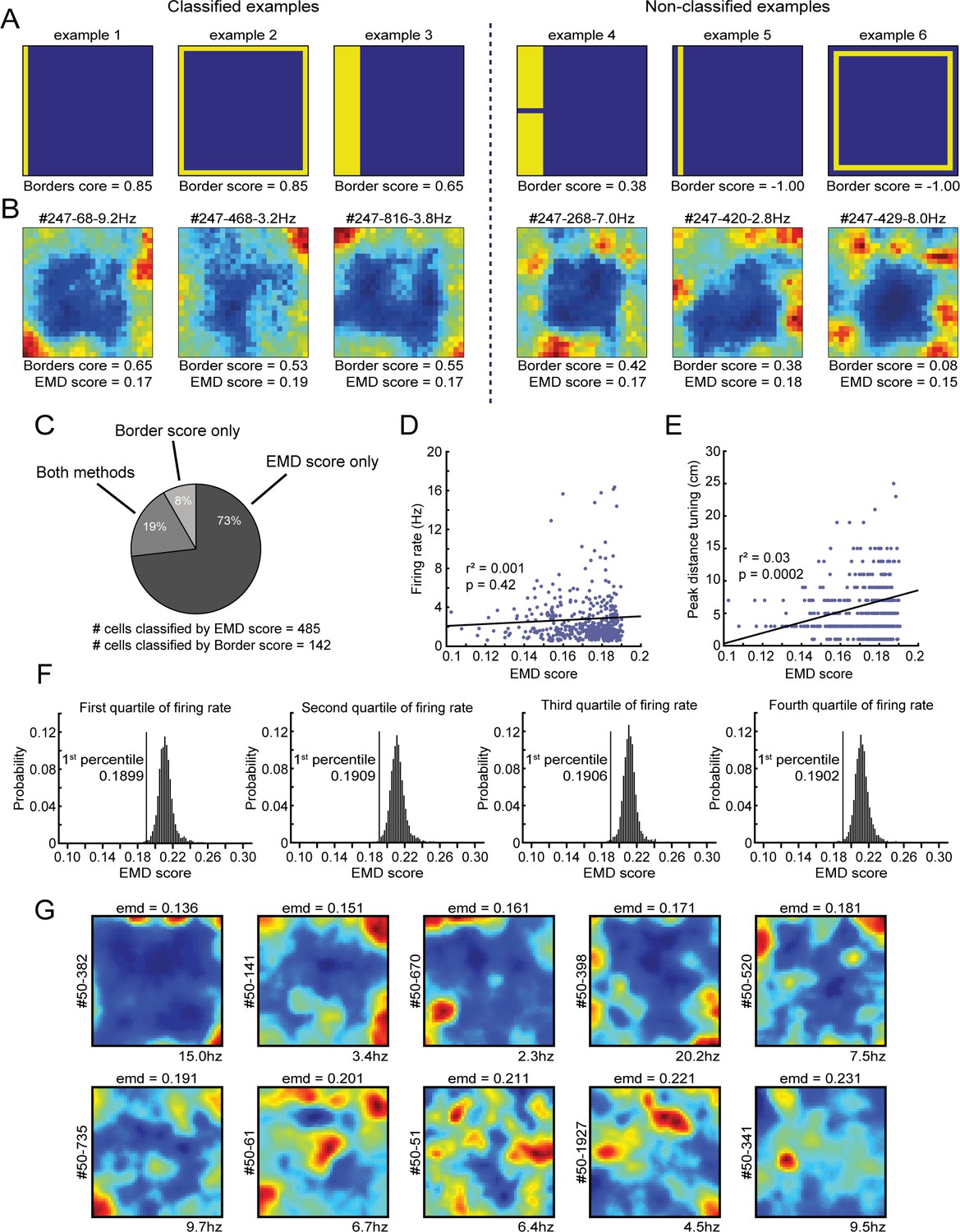
Comparison between the EMD metric and original border score and its relationship with a cell’s firing rate.
(A) Shown are six examples of simulated rate maps and their associated border scores. This metric is designed to capture the coverage of a firing field alongside a single wall, and a maximal score is reached when it occupies only bins that are directly connected to the wall (ex. 1). On the left: three simulated examples of rate maps that would be classified as border cells. On the right: three examples of non-classified rate maps. Extension of a field toward the center lowers the border score (ex. 3), as does breaking the field into two or more subfields (ex. 4). The algorithm is unable to calculate a border score when the firing field does not directly touch the boundary (ex. 5). The border score furthermore does not consider symmetry, as the maximum score on any of the four walls is selected (ex. 2 and 6). (B) Shown on the left are three example RSC border cells that were classified correctly by both the border score (values above 0.5) and our EMD template matching method (values below 0.1906). By contrast, on the right are shown three qualitatively similar RSC border cells that were identified only by the EMD method, as these cells had low, non-significant border scores. RSC border cells tend to form firing fields that are not necessarily connected to the wall, and are often not continuous due to additional directional tuning, leading to low border scores. (C) Distribution and overlap of border cell classification using the border score and EMD methods. (D) No significant correlation exists between a cell’s firing rate and its EMD score. (E) A small correlation (r = 0.17) exists between a border cell’s EMD score and its preferred firing distance, as cells with lower distance tuning are more similar to the boundary template. (F) Four EMD spike-shuffled null distributions, same as in Figure 1E, using rate maps of cells with overall firing rates that fall in one of four quartiles of the total population of neurons. The EMD template matching procedure is robust against differences in the overall spiking rates, where the significant criterion remains at the same cut-off independent of the firing rate of the underlying population of cells included. (G) Spatial rate maps of neurons recorded in RSC of one individual animal with EMD scores at evenly spaced intervals (range: 0.14–0.23). Cells with a score below the value of 0.191 are considered to be border cells.
Figure 1—figure supplement 3
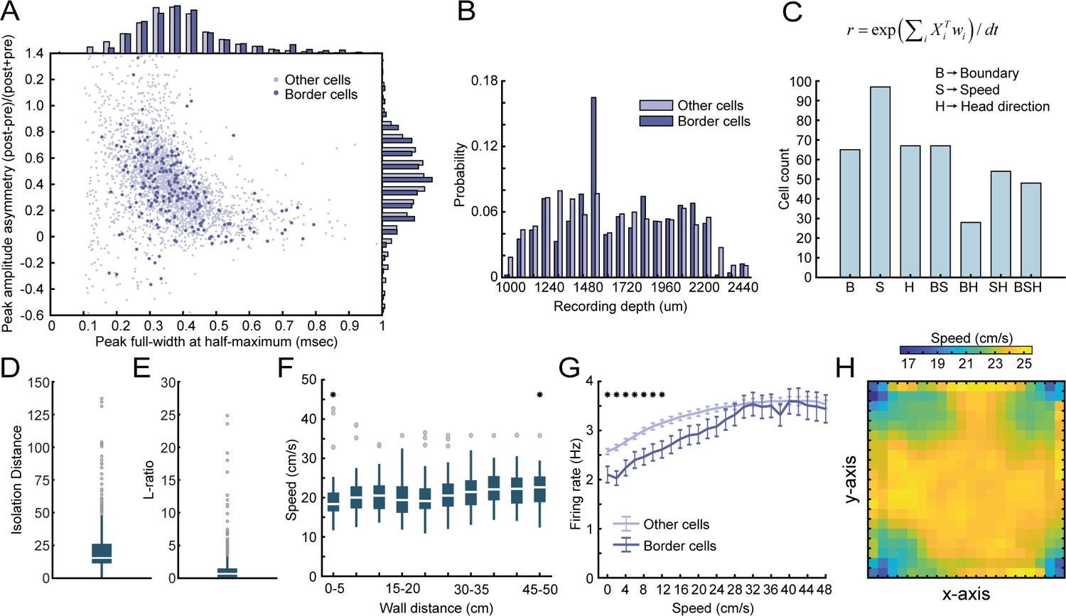
The dissociation between the animal’s running speed and activity around borders.
(A) Waveform properties of RSC border cells versus other cells recorded on the same tetrodes show no major difference between both populations. (B) Border cells were recorded both in granular and dysgranular layers of RSC across the recording depths. (C) An unbiased classification approach was applied based on linear-nonlinear models (Hardcastle et al., 2017). Three variables, Xi, were included: B, a one-dimensional vector of distance to the closest boundary, S, the animal’s running speed, and H, the animal’s allocentric head-direction. Models were built with increasing complexity using a forward-search approach (e.g., starting with one variable, then adding more if the model’s performance increases significantly, tested using ten-fold cross-validation). The model that best explained (e.g., had maximal log-likelihood) the cell’s firing rate, r, using optimal weights, wi, was then selected. Results show that boundary, speed, and head-direction encoding in RSC are independent features, as they can be expressed in isolation, combined with a substantial number of neurons that display conjunctive coding. (D-E) Tetrode cluster quality metrics that quantify the isolation distance (median = 15.39, IQR = 11.26–26.26) and L-ratio (median = 0.67, IQR = 0.17–1.51), based on Kilosort single vector decomposition (SVD) factor loadings (Schmitzer-Torbert et al., 2005). (F) There was no bias in the animal’s behavior around walls, as the running speed of the animals was uniformly distributed as a function of distance to the closest wall. (G) Both border cells and other cells recorded in RSC are modulated by running speed, with a ramping of firing rates as the running speed increases. However, border cells further showed lower firing rates in the low-speed range compared to other recorded cells. (H) Speed of the animal was uniformly distributed across the 2D space of the arena. *p<0.05, Wilcoxon signed-rank test (D), Wilcoxon ranksum test (E).
Figure 1—figure supplement 4
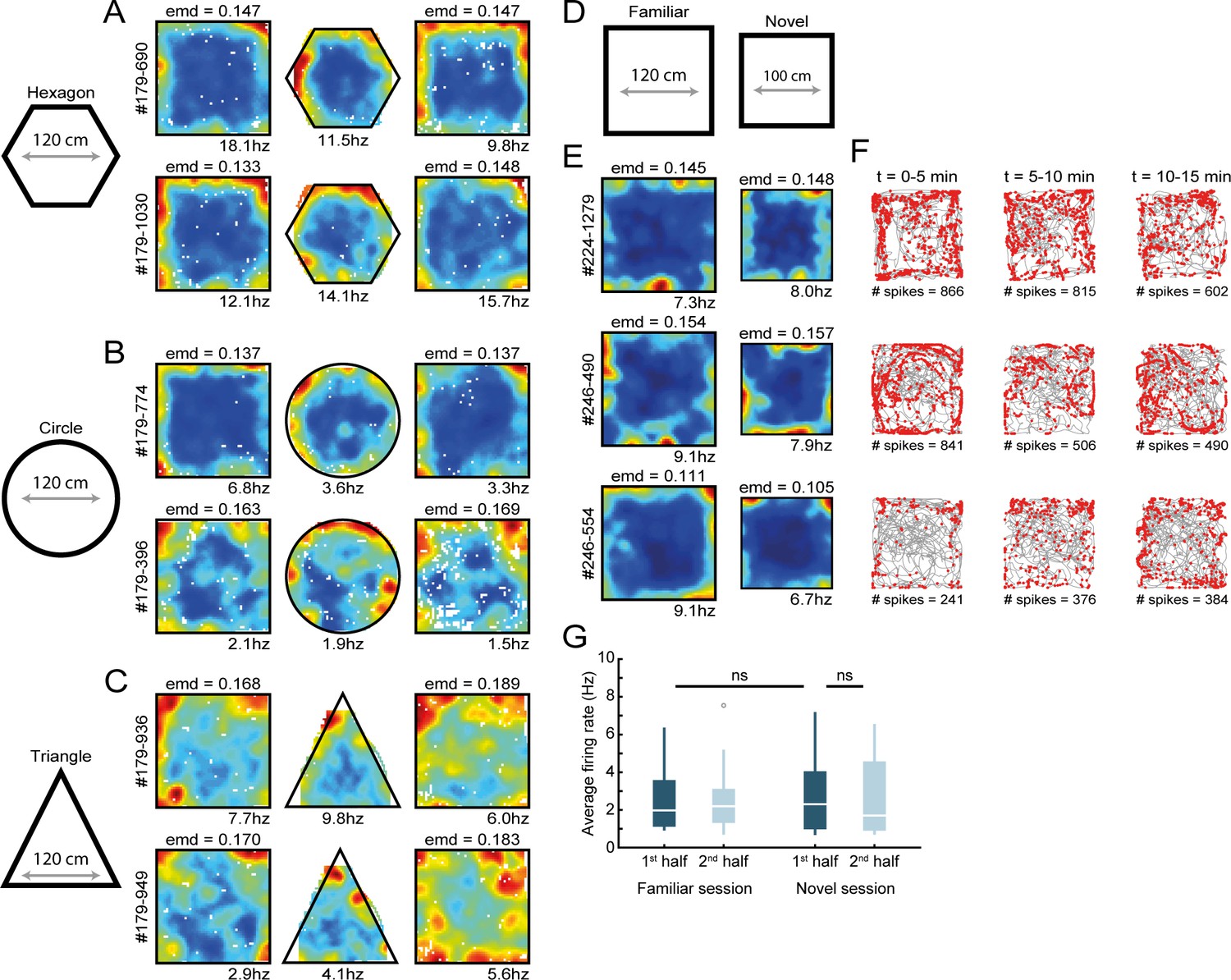
RSC border cell firing under novel conditions and different arena shapes.
(A–C) Recordings were performed across different shapes of environments. Shown are rate maps of border cells that fired at the edge of a squared arena, and cells maintained their firing to the borders when the outer walls were changed to form a hexagonal (A), circular (B), or triangular (C) shape. (D) Several experimental sessions were performed under novel conditions, where animals had never visited neither this maze nor the recording room before. (E) Spatial rate maps of three typical RSC border cells that showed no qualitative differences between a familiar and novel maze. (F) Trajectory spike plots of the novel session for the same cells shown in (E), subdivided into blocks of 5 min. (G) RSC border cells fired with a similar spiking rate already from the beginning of the session, with no significant differences between the familiar and novel sessions. Wilcoxon signed-rank test.
Figure 2
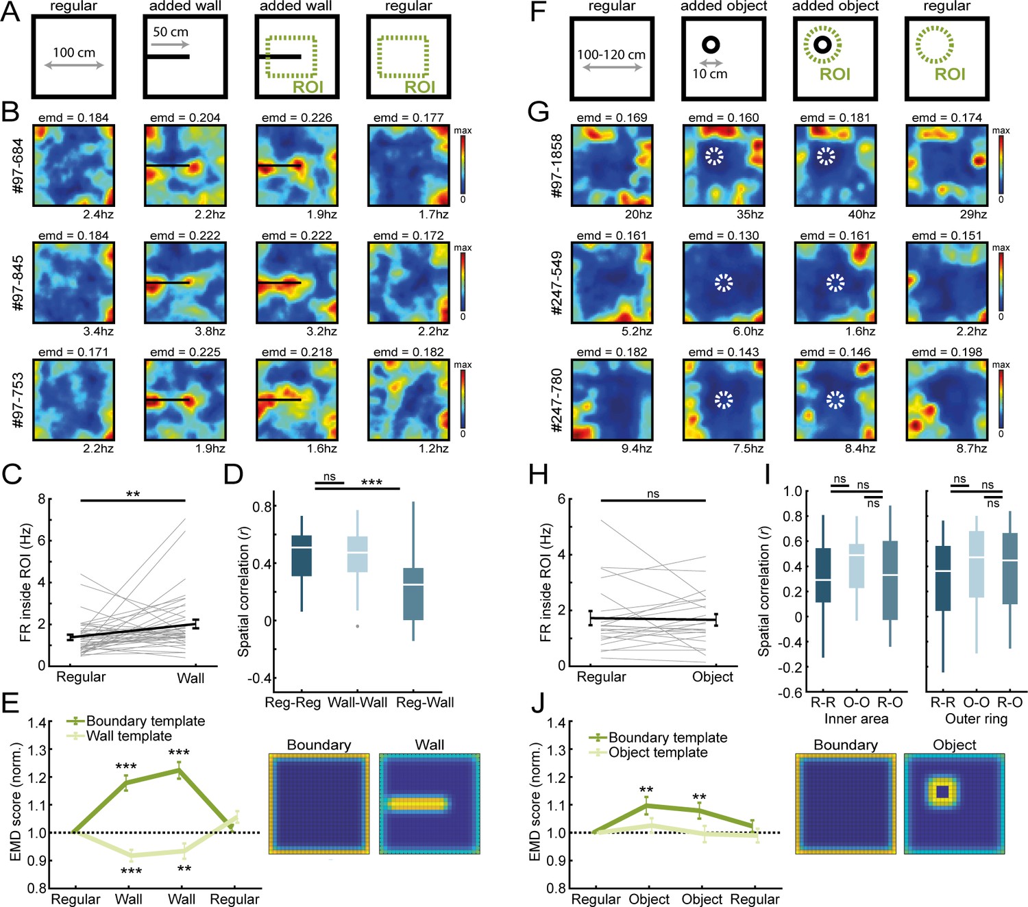
Border cells respond to new walls but not to the addition of new objects.
(A) An additional temporary wall was placed on the maze in the middle sessions. (B) Spatial rate maps of three typical border cells across regular and added wall sessions during one recording day. (C) Border cells formed new firing fields nearby the added wall, as cells significantly increased their firing rate in the region-of-interest (ROI) area around the central wall. (D) Spatial correlations between rate maps of regular and wall sessions were decreased but remained high within session type. (E) Dissimilarity increased for the boundary template as cells formed fields around the added wall, whereas dissimilarity decreased for an added wall template. (F) A new object was introduced either in the north-west corner or the center of the maze. (G) Spatial rate maps of three example border cells across regular and object sessions. (H) Firing rate of border cells in a ROI around the added object remained unchanged between session types. (I) No significant drop was observed in spatial correlations of border cells by the addition of the object. Correlations were split between an outer ring (four rows) and the remaining inner area to isolate activity related to the outer walls versus the object. (J) There was an increase in EMD scores for the boundary template, whereas the spatial rate maps did not fit with the object template either, as their EMD scores remained unchanged. **p<0.01, ***p<0.001, Wilcoxon signed-rank test.
Figure 3 with 1 supplement
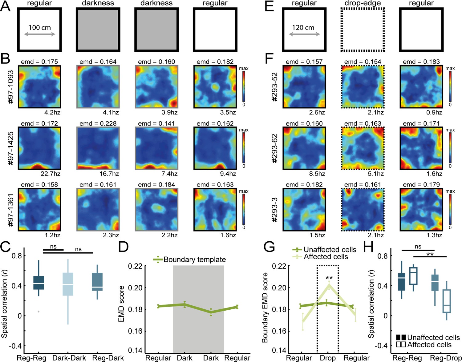
Border coding is maintained in darkness and in the absence of physical walls.
(A) Recordings were performed under no visible light in the middle sessions, and the animal’s position was tracked in the infrared spectrum. (B) Spatial rate maps of three typical border cells recorded in light and dark conditions. (C) Spatial correlations between rate maps of regular and dark sessions remained high, indicating border cells still fired nearby boundaries in darkness. (D) There were no changes in EMD scores with the boundary template, confirming that cells maintained their tuning to the outer walls without direct visual detection. (E) All four outer walls were removed, leaving only a drop-edge to confine the arena. (F) Spatial rate maps of three example border cells across recording sessions. (G) Spatial rate maps were maintained for a majority of border cells (unaffected) but a subset of neurons showed disrupted firing near the drop-edge that resulted in an increase in the EMD score on the boundary template (affected). (H) Spatial correlations between rate maps of regular and drop-edge sessions remained high for the unaffected cells but decreased significantly for the affected cells. **p<0.01, Wilcoxon signed-rank test.
Figure 3—figure supplement 1

Control experiments to assess the role of somatosensory information in computing border information.
(A) Whiskers of rats were trimmed to the skin on the final recording day, with one behavioral session before and after trimming for each animal. (B) Example rate maps of RSC border cells before (left column) and after trimming (right column), with four examples of cells that were unaffected by trimming and maintained their boundary tuning the in absence of whiskers. No significant changes were observed in the proportion of border cells due to whisker trimming. (C) Whisker trimming had no significant effect on the overall firing rates of RSC border cells. (D) Recordings were performed from neurons in the barrel field of the primary somatosensory cortex (S1bf) by implanting a 64-channel silicon probe. (E) In an anesthetized preparation, an object (sandpaper) was moved through the whiskers contralateral to the recorded hemisphere at 10 s intervals. The silicon probe was lowered until a substantial number of cells responded consistently to the whisker stimulation. (F) A subset of neurons fired reliably after whisker stimulation. Top: example raster plot of spikes from a representative whisker-responsive cell. Bottom: number of spikes for individual neurons (colored lines) and the population-average (black line) shows that neurons fired 30–500 ms after the object moved through the whiskers. (G) Recordings were performed across four behavioral sessions, with an object introduced to the maze in the middle two sessions. Shown are rate maps of four example cells recorded from S1 barrel cortex that matched our border cell criteria, where cells fired around the edges of the arena but also formed firing fields around the object. (H) EMD scores confirm that S1bf cells fired around objects, as the boundary EMD scores increased significantly in the object session, while the object template EMD scores decreased accordingly. (I) Spatial correlations between rate maps of regular and object sessions decreased significantly when comparing the inner area of the rate map, consistent with the formation of firing fields around the object. **p<0.01, ***p<0.001, Wilcoxon signed-rank test.
Figure 4 with 2 supplements
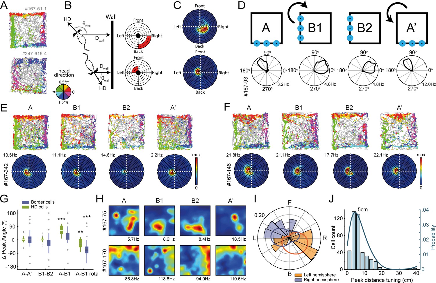
Egocentric tuning of RSC border cells has a hemispheric bias and is invariant to the rotation of place and head-direction signals.
(A) Example trajectory spike plots with spike locations color-coded according to the head-direction of the animal. Most spikes alongside a wall occur only when the animal was in a narrow range of directions. Top: recorded in the right hemisphere. Bottom: recorded in the left hemisphere. (B) Trajectory data was projected onto new body-centric border maps, where coordinates indicate the distance (Dwall) and direction (θwall) of the closest wall relative to the animal's position and head-direction (HD), respectively. (C) Rate maps in this border space for the same example cells shown in (A). (D) Top: Blue LEDs were placed as distal cues on one side of the maze, and the entire experimental set-up was rotated 90° clockwise in the middle sessions. Bottom: example allocentric HD cell showing its tuning shifted accordingly. (E-F) Two example border cells with trajectory spike plots and border rate maps showing egocentric border tuning was stable across rotation sessions. (G) Comparison of shifts in direction tuning for allocentric head-direction cells and egocentric border cells across the different sessions, where B1-rota is a rotated version of the rate map in the opposite direction of the physical rotation of the arena, matching the layout again as in A. (H) Two examples of spatially-stable cells, defined as having spatial correlations above the 99th percentile of a time-shuffled distribution, which rotated along with the cue. (I) Preferred directional tuning of all recorded border cells with significant directional tuning, split according to the location of the electrode in either the left or right hemisphere. (J) Preferred distance tuning of all RSC border cells. **p<0.01, ***p<0.001, Wilcoxon signed-rank test.
Figure 4—figure supplement 1

Directional and distance tuning properties of RSC border cells.
(A) Venn diagram showing the overlap between cells that display distance tuning (classified using the EMD scores) and cells with egocentric directional tuning to walls (classified using the egocentric boundary MVL). (B) Distribution of MVL values and EMD scores for cells that are significantly tuned to the distance or direction to the boundaries. (C) Simulated EMD scores of rate maps with synthetic spikes at specific distances away from the wall, simulated at 2 cm intervals using all behavioral sessions. Mean across cells (thick line) ± SEM (shaded). (D) EMD classification of RSC border cells with a subset of data and different templates, each with firing fields at increasingly further distances from the wall. Most original cells could be captured using templates with fields up to 12 cm away (template 3), and although higher templates found several additional cells, no major new populations of border cells were found using far-distance templates. This confirms that most border cells in RSC exhibit distance tuning at close wall proximity below the range of 20 cm.
Figure 4—figure supplement 2
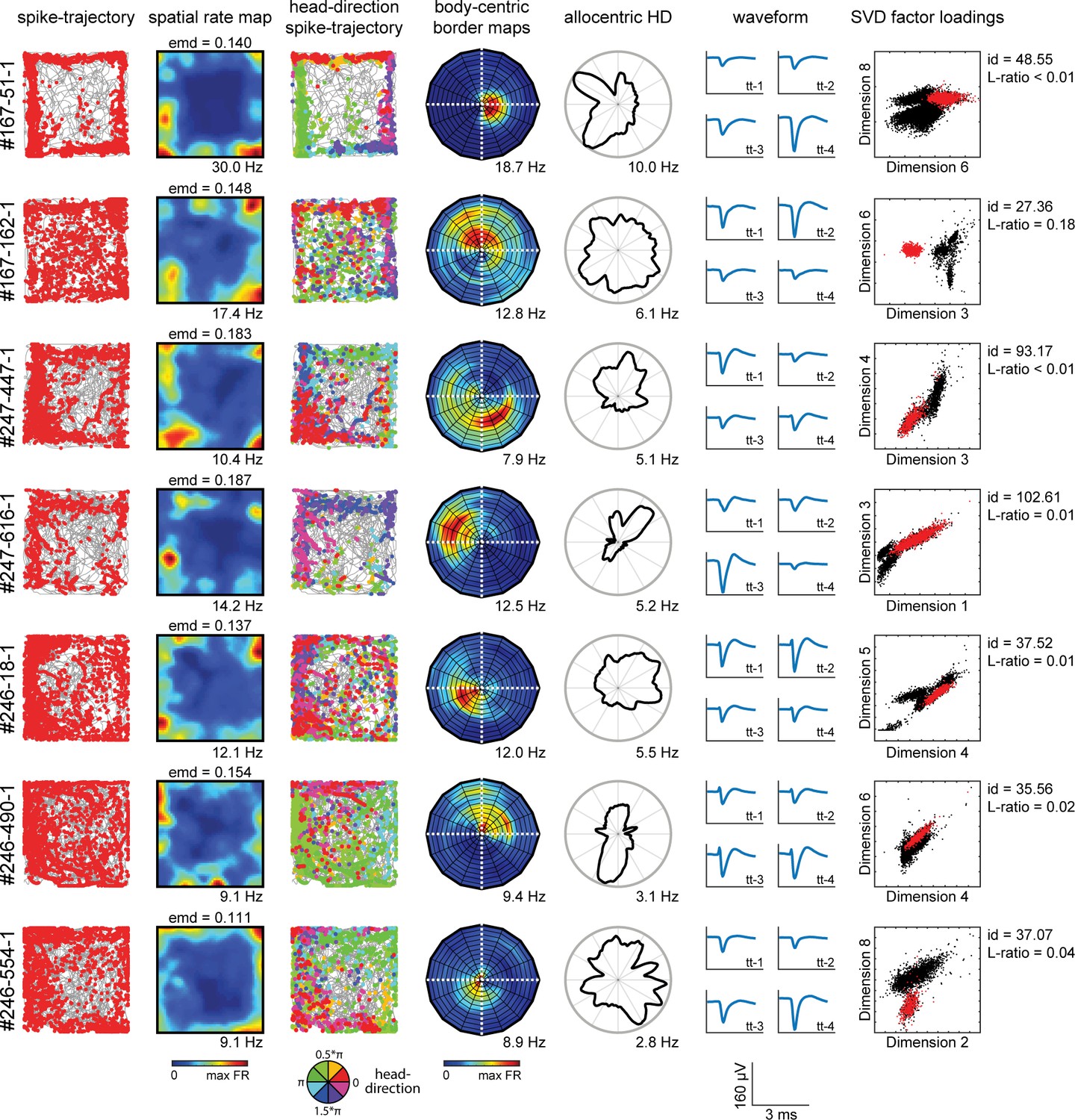
Neuron cluster properties along behavioral axes.
Shown are example cells (one per row) with their firing properties across multiple behavioral variables, together with their cluster properties obtained during spike sorting. First column: trajectory spike plots with the animal’s trajectory (gray line) and his position in space (red dots) at the time of spiking. Second column: color-coded spatial rate map, with warm colors indicating higher firing rate. Third column: head-direction trajectory spike plots, with colored dots indicating the head-direction of the animal at time of spiking. Fourth column: body-centric border rate maps, showing the firing rate with respect to the distance and direction of the boundary relative to the animal. Fifth column: firing rate as a function of allocentric head-direction. Sixth column: cluster waveforms across four channels of the main tetrode. Seventh column: cluster factor loadings on two distinctive SVD factors used for cluster cutting during spike sorting in the Kilosort algorithm. Cluster quality metrics show isolation distance (id) and L-ratio (Schmitzer-Torbert et al., 2005).
Figure 5 with 4 supplements

Sharp boundary tuning of RSC border cells relies on input from MEC.
(A) An AAV encoding inhibitory DREADDs hM4Di was injected into MEC while tetrodes were positioned in RSC. Scale bar, 1 mm. (B) Four tetrodes were placed locally near the virus injection site, showing a subset of affected MEC neurons that decreased their activity 10–15 min after subcutaneous administration of agonist-21 (DREADDs agonist). (C) Two example RSC border cells that were affected by MEC inhibition and lost their spatial tuning. (D-E) Border cells in RSC exhibited increased EMD scores as well as lower firing rates after inhibition of MEC. Gray lines indicate individual cells. (F) Reversed experiment, with electrophysiological recordings in MEC while the AAV was injected into RSC. Scale bar, 1 mm. (G) A subset of RSC neurons decreased their activity after the administration of agonist-21. (H) Two example MEC border cells that were unaffected by inhibition of RSC. (I-J) Border cells in MEC did not show any significant qualitative changes in border tuning or firing rates after RSC inhibition. Gray lines indicate individual cells. (K) An AAV encoding inhibitory Halorhodopsin channels was injected into MEC, while an optrode with tetrodes and optic fiber was implanted in RSC to inhibit MEC axons. Scale bar, 1 mm. (L) Two example border cells in RSC that showed disrupted border tuning during inhibition of MEC terminals near the recording site. (M) A retroAAV encoding red-shifted inhibitory Cruxhalorhodopsin (Jaws) channels was injected into RSC together with the implantation of a 64-channel silicon-probe, while an optic fiber was placed at the dorsal edge of MEC for the silencing of cells that project to RSC. Histology shows the expression of the virus in neurons located in deep layers of MEC. Scale bar, 1 mm. (N) Two examples of RSC border cells that were disrupted due to optogenetic silencing of RSC-projecting neurons in MEC. (O) RSC border cells showed disrupted border tuning on a population-level as a direct result of MEC inhibition, both when silencing RSC-projecting neurons in MEC as well as during local inhibition of their axon terminals near the recording sites in RSC. *p<0.05, **p<0.01, ***p<0.001, Wilcoxon signed-rank test.
Figure 5—figure supplement 1

Tetrode locations and hM4Di expression in the experiments of DREADDs-mediated inactivation.
Left: Nissl-stained sections and fluorescent images from individual animals used for the DREADDs experiments. In rat #169 and #170, recordings were performed from bilateral MEC and AAV (AAV8-hSyn-hM4Di-mCherry) was injected into the right RSC. Sagittal sections are shown for both Nissl-stained and fluorescent images. Positions of tetrode tracks are indicated by red circles. In rat #171 and #217, recordings were performed from the right RSC, and the AAV was injected into bilateral MEC. Coronal sections are shown for Nissl-stained images, and sagittal sections are shown for fluorescent images. Right two columns: the left plots show normalized firing rates of cells recorded from the virus injected site. The DREADDs agonist-21 was injected at the beginning of the recording sessions. Two red traces show representative cells that exhibited a significant reduction of firing rates after the injection (p<0.05, Wilcoxon ranksum test for rate changes between 0–10 min and 30–40 min), and blue traces are cells that were not significantly affected by the drug. The activity of cells was partly disrupted by the agonist-21 administration, as 70% (14/20) of the recorded cells near the injection site in RSC significantly reduced their firing rates to 53.0 ± 6.4% of their baseline firing, whereas 59% (26/44) of the MEC cells decreased their spiking rate to 47.2 ± 5.5% of baseline. The right plots show the probability density of the animal’s running speed during random foraging in the open field arena, before and after the drug injection. DREADDs-mediated inactivation did not significantly affect the animal’s running speed (p>0.05 in Friedman test). Each plot shows mean (solid lines) and SEM (shaded).
Figure 5—figure supplement 2
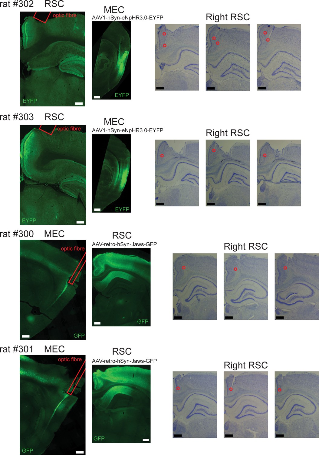
Recording locations and virus expression in the experiments of optogenetic inactivation.
Left: Fluorescent images from individual animals used for the optogenetic experiments. Right: Nissl-stained coronal sections of RSC where recordings were performed. In rat #302 and #303, an AAV encoding inhibitory Halorhodopsin chloride pumps (eNpHR3.0) was injected into MEC in the right hemisphere. Coronal sections of RSC and sagittal sections of MEC show virus expression in MEC cell bodies and their axon terminals that terminate in superficial layers of RSC. Recordings were performed in RSC using tetrodes, together with an optic fiber that allowed for axon-terminal inhibition. In rat #300 and #301, a retroAAV encoding red-shifted Cruxhalorhodopsin chloride pumps (Jaws) was injected into RSC in the right hemisphere. Sagittal sections of MEC shows virus expression specifically in deep layers of MEC. Recordings were performed in RSC using a 64-channel silicon probe, while an optic fiber was located at the dorsal edge of MEC to silence MEC cells with projections to RSC. Due to the decay of light intensity, laser light likely reached only the dorsal pole of MEC, leaving the ventral parts largely unaffected. Laser light was turned on in the middle sessions, following an A-B-A’ protocol.
Figure 5—figure supplement 3
Additional analyses for optogenetic experiments.
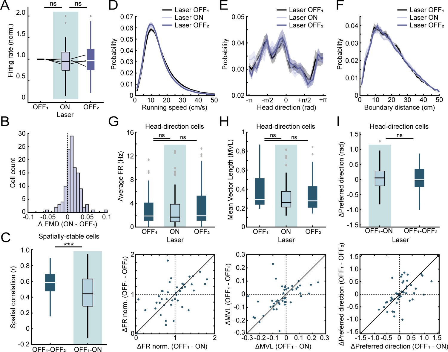
(A) Optogenetic inactivation of MEC neurons that project to RSC had no effect on border cell firing rates in RSC. Black lines indicate individual animals. (B) Distribution of changes in EMD scores in RSC border cells between ratemaps of the laser OFF and ON session, showing a positive shift in scores across the population of neurons during optogenetic inhibition of MEC input. (C) Spatially-stable cells in RSC (n = 83 spatial cells), classified with spatial correlations between rate maps of both laser OFF sessions above the 99th percentile of a shuffled distribution that were not border cells, were affected by inhibition of MEC, leading to lower spatial correlations with laser light on. (D-F) Inhibition of MEC did not result in any observable changes in the animal’s behavior, with no changes in the running speed (D), head-direction (E) nor distance to the nearest boundary (F). (G-I) Cells tuned to allocentric head-direction were present in both MEC and RSC, but inhibition of MEC neurons had no effect on head-direction tuning of HD cells in RSC (n = 47 head-direction cells). There was no change in average firing rates (G), tuning strength expressed as MVL (H), nor a shift in the preferred direction of the cell’s tuning curve (I). ***p<0.001, Wilcoxon signed-rank test.
Figure 5—figure supplement 4
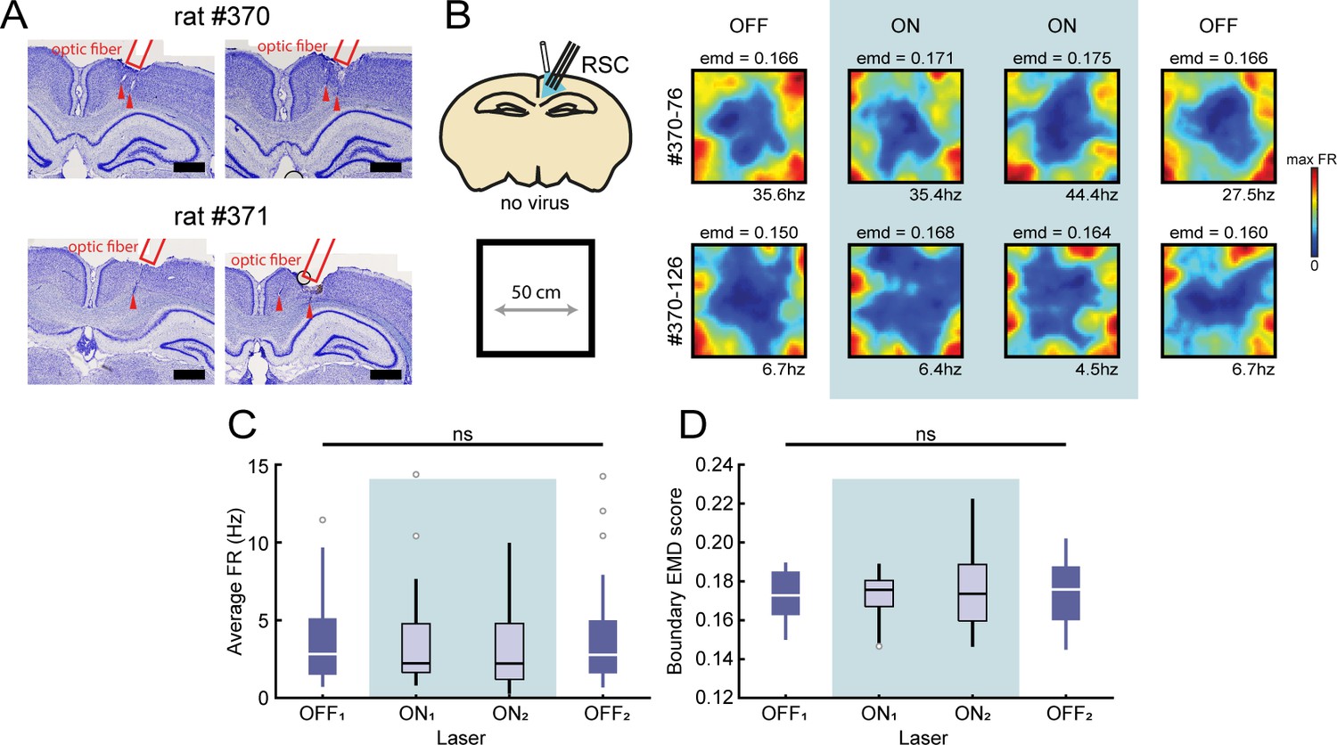
Boundary coding was stable during the laser application without opsin expression.
(A) Nissl-stained coronal sections of two control animals showing the location of the implanted optrodes in right RSC. Scale bar, 1 mm. (B) In order to account for non-specific manipulation effects such as tissue heating, no inhibitory opsins were expressed for two control animals while exposing the recorded neurons to laser light under the same conditions as for Figure 5. Animals foraged freely in an open field arena during the experiment. Shown are two representative border cells in RSC that displayed stable firing patterns near boundaries of the arena, independent of the presence of laser light. (C) The population of recorded RSC border cells showed no changes in their FR across session type (Friedman test: X2(3)=2.64, p=0.45). (D) RSC border cells showed stable EMD scores across all sessions and did not suffer disrupted border tuning when applying laser light in the absence of inhibitory opsins (Friedman test: X2(3)=5.44, p=0.14).
Figure 6 with 1 supplement

Firing of RSC border cells provides local boundary information and is correlated with the animal’s future motion.
(A) Spike trajectory plots and spatial rate maps of typical border cells recorded in RSC and MEC. (B) Proportion of border cells in RSC and MEC that had significant directional tuning to allocentric head-direction or egocentric boundary-direction. (C) A decoder using a support vector machine (SVM) classifier estimated the animal's distance to the wall based on population spiking activity. Local distance information was present in both regions but extended further into the center of the arena only in MEC. (D) Self-motion maps were computed based on short trajectories of the animal, giving lateral and frontal displacements (Δx and Δy, respectively) and distance traveled, Dist, in 100 ms time bins relative to the animal’s forward head-direction, giving a self-centered moving direction, θm, at each timepoint. (E) Example motion map of an RSC border cell with spike times shifted in time relative to the animal’s motion data. A firing field emerged on left turns when spikes were shifted −200 to −500 ms before motion. (F) RSC border cells fired prospective to motion, where the amount of information present in motion maps is maximal when spike timings were shifted −50 to −300 ms earlier. (G) MEC border cells by contrast did not show any prospective or retrospective activity. (H) Spike-triggered average of changes in direction, calculated as the difference of moving directions in 250 ms bins, where positive values indicate right turns. RSC spikes preceded turning behavior of the animal by ~200 ms, with border cells in opposing hemispheres firing prospectively to ipsilateral turns. (I) MEC spikes by contrast were not locked to any change in the animal’s behavior. *p<0.05, t-test.
Figure 6—figure supplement 1
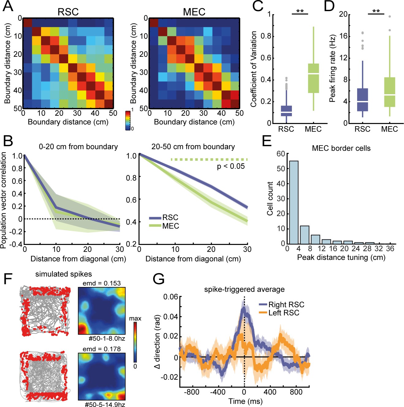
Additional population analysis on RSC and MEC border cells.
(A) Population vector correlation of firings rates, binned according to the wall distance for border cells in RSC (left) and MEC (right). (B) Population vector correlations decay from the diagonal to distal bins at a similar rate for MEC and RSC border cells in the small wall-distance range of 0–20 cm. In the larger distance range, decay is stronger for MEC, which suggests more heterogeneity in firing across the population, allowing for discrimination of the wall distance to a large extent. (C) Coefficient of variation (CV) between average firing rates alongside each wall for RSC and MEC border cells. (D) Border cells in MEC exhibited higher peak firing rates compared to RSC. (E) Distribution of peak distance tuning for MEC border cells. (F) Simulated spiking data using real behavioral position data. Spikes were generated based on a non-uniform Poisson distribution and selected from time points where the animal was both located between 5 and 20 cm distance of a boundary (randomly selected for each cell), and had a specific orientation toward the wall (width = 0.5*π, shifted by 90° for each neighboring wall to maintain consistent wall orientations). Shown are examples of trajectory spike plots and their associated spatial rate maps of two simulated cells. (G) Spike-triggered average of changes in moving direction using simulated spiking data. Data included all behavioral sessions used for Figure 6H, and an identical number of artificial cells as those recorded in each session were generated. Simulated cells did not show prospective activity before a change in direction, as the original peak at +200 ms disappeared. **p<0.01, Wilcoxon ranksum test.
Author response image 1

EMD classification of border cells in MEC using MEC-specific templates.
(A) Distribution of EMD scores, selecting the lowest value on any of the four templates for each MEC neuron. Dark green represents the population of border cells in MEC that were classified previously using the border score. (B) The four templates used in this procedure, with firing fields attached to a single wall. (C) Spatial rate maps of 8 cells with the lowest EMD score on any of the templates (e.g., most left values in A). Top row: two examples of cells with localized firing nearby the wall, which resulted in a low EMD score. Middle row: three examples of cells not classified by the border score (e.g. values below 0.5), but still rather border-like. Bottom-row: three border cells identified by both methods.
Author response image 2
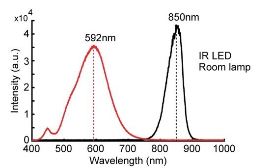
Spectral density measures of the light used in the experiments, captured by a Flame-S spectrometer (OceanOptics).
The black line represents the spectral component of the infra-red LED used for tracking during darkness, while the red line shows components of the desk lamp used to create dim light conditions. Intensity unit sizes are arbitrary, with the sensor kept at a distance of the light source as to not saturate it.
Author response image 3

Firing rate of border cells inside the object ROI between the first and last regular session without an object present.
Individual cells (grey lines) show both increased and decreased firing, but no mean difference was found between the sessions, as expected (First regular, FR = 1.61 ± 0.23; Last Regular, FR = 1.50 ± 0.29; Wilcoxon signed rank test: z = -0.763, p = 0.45).
Additional files
Download links
A two-part list of links to download the article, or parts of the article, in various formats.
Downloads (link to download the article as PDF)
Open citations (links to open the citations from this article in various online reference manager services)
Cite this article (links to download the citations from this article in formats compatible with various reference manager tools)
Entorhinal-retrosplenial circuits for allocentric-egocentric transformation of boundary coding
eLife 9:e59816.
https://doi.org/10.7554/eLife.59816


