Drift and termination of spiral waves in optogenetically modified cardiac tissue at sub-threshold illumination
- Research Group Biomedical Physics, Max Planck Institute for Dynamics and Self-Organization, Germany
- Institute for the Dynamics of Complex Systems, Goettingen University, Germany
- German Center for Cardiovascular Research, Partner Site Goettingen, Germany
- University Medical Center Goettingen, Clinic of Cardiology and Pneumology, Germany
- European Laboratory for Non-Linear Spectroscopy, Italy
- Division of Physiology, Department of Experimental and Clinical Medicine, University of Florence, Italy
- Department of Physiology, MGill University, Canada
- Institute for Experimental Cardiovascular Medicine, University of Freiburg, Germany
- National Institute of Optics, National Research Council, Italy
- INPHYNI, CNRS, Sophia Antipolis, France
- University Medical Center Goettingen, Institute of Pharmacology and Toxicology, Germany
Figures
Figure 1 with 1 supplement
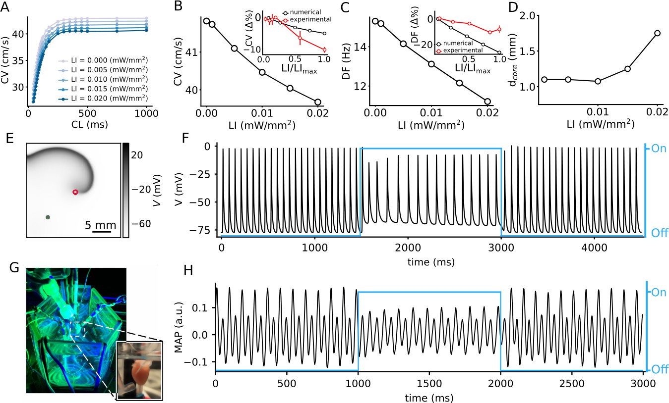
Effect of sub-threshold illumination on in silico optogenetically modified adult mouse ventricular tissue.
(A) Conduction velocity (CV) restitution at different light intensities (LIs). (B) CV decreases with increase in LI, for electrical excitation waves paced at 5 Hz. Inset shows a comparison of the reduction of CV in experiments (red) and simulations (black) at different LI, relative to the unilluminated planar wave (CV reported as mean ± SEM, N = 4 with 12 trials). (C) Dominant frequency (DF) of a spiral wave decreases with increase in LI. Inset shows a comparison of the reduction of DF in experiments (red) and simulations (black) at different LI, relative to the unilluminated spiral (DF reported as mean ± SD, N = 2 with 14 trials). (D) Increase in diameter of the spiral wave core () with increase in LI. Here, core represents the circle that encloses one cycle of the spiral tip trajectory in the stationary state. (E) A representative snapshot of the spiral wave in a 2D simulation with a circular trajectory shown with red marker. The green marker indicates the location for extraction of the voltage timeseries in (F). (G) Our set-up of the intact mouse heart from which monophasic action potential (MAP) recordings in (H) were made. The blue traces in (F) and (H) illustrate the status of illumination (on/off) during the simulation or experiment.
Figure 1—figure supplement 1
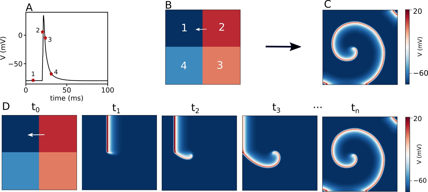
Protocol for inducing a spiral wave in 2D.
(A) Four different membrane voltage values are chosen; one value from resting state (1), one value from depolarization state (2), and two values from repolarization state (3 and 4). (B) The 2D mono-domain (200 × 200 grid points) is initialized by four selected values. (C) A spiral wave is formed. (D) A series of frames during formation of the spiral wave.
Figure 2 with 1 supplement

Spatial drift of a spiral wave imposed by a gradient of sub-threshold illumination.
(A) Trajectory of a drifting spiral tip in a domain with an illumination gradient ranging from LI = 0 mW/mm2 at the left boundary to LI = 0.01 mW/mm2 at the right boundary. Colors indicate different times, here and B-F. (B) Time evolution of the voltage distribution along the dashed line indicated in (A), in a quiescent domain with the same LI gradient. (C) Spatial derivative of the voltage distribution () along the dashed line in (A), at different times, for the same applied LI gradient as in (A–B). (D)-(F) show plots corresponding to (A)-(C), but for an LI gradient ranging from 0 to 0.02 mW/mm2. In this case, the spiral drifts all the way to the right boundary, within the given time frame, and terminates itself. The inset in (D) shows a portion of the cycloidal tip trajectory of the spiral. (G) Timeseries of the tip speed (red) and curvature of the spiral tip trajectory (black), as the spiral drifts along the LI gradient (green band) or against it (gray band). The profiles correspond to the part of the trajectory shown in the inset of panel D. (H) Increase in the maximum horizontal displacement (d) of the spiral core, with increase in the applied LI gradient (in mW/mm3), within the given time frame (2 s) of the simulation (displacement reported as mean ± SD, N = 10).
Figure 2—figure supplement 1
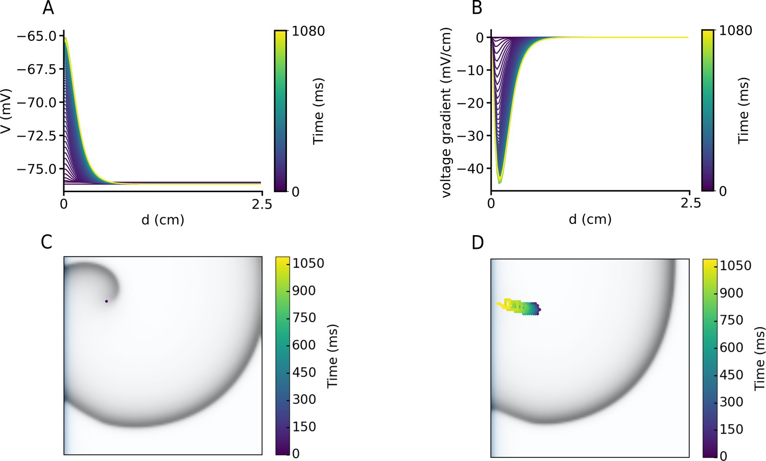
Spatial drift of a spiral wave imposed by a exponential pattern of sub-threshold illumination.
(A) Time evolution of the voltage distribution along a line perpendicular to the illumination pattern in a quiescent domain. (B) Spatial derivative of the voltage distribution () along the line perpendicular to the illumination pattern in a quiescent. (C) Initial position of the spiral tip in a domain with an illumination gradient ranging from LI = 0 mW/mm2 at the left boundary to LI = 0.07 mW/mm2. (D) Drift of the spiral wave toward the region with higher LI.
Figure 3
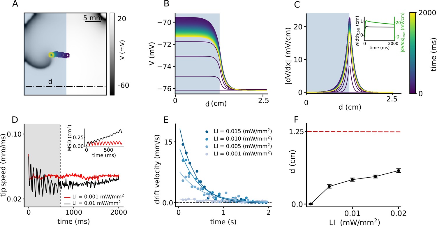
Spatial drift of a spiral wave in a domain that is partially illuminated with sub-threshold LI.
(A) Trajectory of the spiral wave tip, as it drifts from the non-illuminated region to the region illuminated with LI = 0.01 mW/mm2. Colors indicate different times, here and B-C. (B) Time evolution of the voltage distribution along the dashed line indicated in (A), in a quiescent domain with the same illumination. (C) Spatial derivative of V () along the dashed line in (A), at different times, for the same illumination as in (A–B). Inset shows the time evolution of the distribution of at the interface between the illuminated and non-illuminated regions. The green curve shows the timeseries of the peak , whereas the black curve shows the corresponding timeseries for the width of the distribution in (C). We defined ’width’ as the horizontal distance between two points in the domain where . (D) Timeseries of the spiral tip speed at LI = 0.001 mW/mm2 (red) and 0.01 mW/mm2 (black). Inset shows the mean square displacement profiles corresponding to the first 800 ms of illumination, shaded gray in the speed plot. (E) Timeseries of the drift speed of the spiral core at LI = 0.001 (gray), 0.005 (light blue), 0.01 (dark blue), and 0.015 mW/mm2 (indigo). We observe that for any LI, drift speed decreases exponentially with time as the spiral core crosses the interface. (F) Slow increase in the maximum horizontal displacement (d) of the spiral core, with increase in LI applied to one half of the domain (displacement reported as mean ± SD, N = 10).
Figure 4
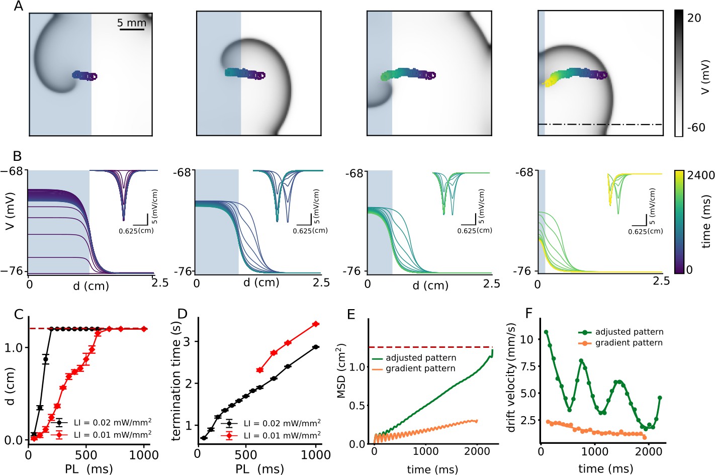
Continuous spatial drift of a spiral wave using a multi-step adjusted pattern illumination protocol.
(A) Trajectory of the spiral wave tip, during different steps of the illumination protocol. (B) Time evolution of the voltage distribution and its spatial derivative (inset) for each step of the protocol, as measured along the dot-dashed line shown in the last sub-figure of panel (A). (C) Horizontal displacement d of the spiral wave core at LI = 0.01 (red) and 0.02 (black) mmW/mm2, respectively, at different pulse lengths (PL) (displacement reported as mean ± SD, N = 10). (D) Termination time for the cases in which the spiral drifted all the way to the boundary and annihilated itself through collision. Red and black curves represent data for LI = 0.01 mW/mm2, and 0.02 (black) mW/mm2, respectively (termination time reported as mean ± SD, N = 10). (E) Mean squared displacement of the spiral wave core with two different illumination protocols: multi-step adjusted pattern (green) and gradient pattern (orange). (F) Drift velocity of the spiral wave core for each case of illumination patterns, multi-step adjusted pattern (green) and gradient pattern (orange).
Author response image 1
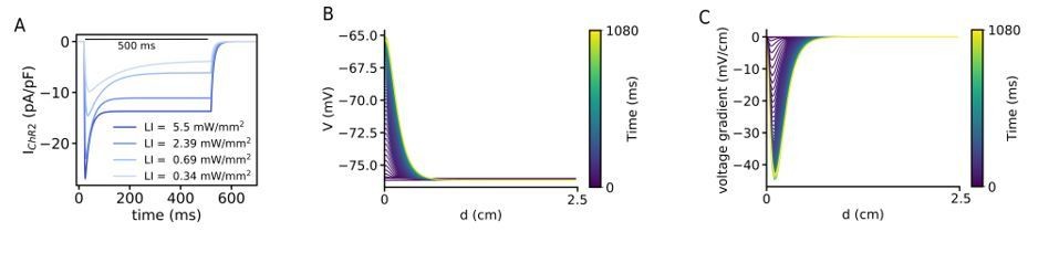
(A) Kinetics of the ChR2 current at different LI. All cases shows an initial peak which decays to the steady-state and when the light turns off decays to the baseline. (B) Time evolution of the voltage distribution along the illumination pattern with an exponential decay in a quiescent domain with the LI of 0.07 mW/mm2. (C) Spatial derivative of V (dV/dx) along the illumination pattern with an exponential decay at different times, for the same illumination as in (A).
Author response image 2

(A) It indicates the action potentials at 15 different points at the domain with a linear gradient pattern when a planar wave propagates through the domain perpendicular to the illumination pattern, shown in (B). The inset shows an increase of APD75 along the illumination gradient showing the non-uniformity of the refractory period along the gradient.
Videos
Video 1
Spatial drift of the spiral wave imposed by an LI gradient of 8 × 10⁴ mW/mm3.
The spiral wave drifts along the illumination gradient direction. Finally the spiral wave collides to the boundary and is terminated.
Video 2
Spatial drift of the spiral wave in a domain that is partially illuminated with LI of 0.01 mW/mm2.
Initially, the spiral wave drifts fast toward the uniformly illuminated region, then it slows down due to the homogeneous region far from the interface of the illuminated and non-illuminated regions.
Video 3
Continuous spatial drift of a spiral wave using a multi-step adjusted pattern illumination with LI of 0.01 mW/mm2.
At each step of reducing the size of the illuminated region, the illumination was applied with a constant illumination PL of 600 ms. The spiral wave drifts continuously along with the reduction direction of the illuminated region size. Finally it collides to the boundary and is terminated.
Video 4
Drift of a spiral toward the illuminated region with an exponential decay pattern with LI 0.07 mW/mm2.
Video 5
A spiral wave rotation with no illumination pattern.
Tables
Table 1
Comparison between calculated drift-induced displacement of the spiral wave (calculated d), and the observed maximum displacement (d) at different LI, for the single-step illumination pattern.
| LI (mW/mm2) | V0 (mm/s) | τ (s) | Calculated d (cm) | D (cm) | Tolerance (%) |
|---|---|---|---|---|---|
| 0.001 | 1 | 1.1 | 0.09 | 0.09 | 0 |
| 0.005 | 8 | 0.49 | 0.375 | 0.39 | 4 |
| 0.010 | 14 | 0.39 | 0.477 | 0.53 | 11 |
| 0.015 | 20 | 0.35 | 0.55 | 0.66 | 22 |
Table 2
Key resource table for bench research involving the intact mouse heart (for studying the arrhythmia frequency).
| Reagent type | Designation | Source | Additional information |
|---|---|---|---|
| Biological sample | Transgenic mouse heart expressing ChR2 | Dr. S. Sonntag, PolyGene AG, Switzerland | Isonated form transgenic mouse (α-MHC-ChR2) |
| Chemical compound, drug | Di-4-ANBDQPQ stain | AAT Bioquest | Red-shifted voltage-sensitive dye to optically probe membrane potentials |
| Software, algorithm | AcqKnowledge | BIOPAC Systems, Inc | Software for Data Acquisition and Analysis |
Table 3
Key resource table for bench research involving the intact mouse heart (for studying the conduction velocity).
| Reagent type | Designation | Source | Additional information |
|---|---|---|---|
| Biological sample | Transgenic mouse heart expressing ChR2 | Prof. Marina Campione, University of Padova, Italy | Isolated from transgenic mouse (ChR2-MyHC6-Cre+) |
| Chemical compound, drug | Di-4-ANBDQPQ stain | Prof. Leslie M. Loew, Center for Cell Analysis and Modeling, UConn Health, Farmington (USA) | Red-shifted voltage-sensitive dye to optically probe membrane potentials |
| Software, algorithm | LabVIEW 2015 (64-bit) software HCImageLive software camera | National Instruments, Austin, TX, USA Hamamatsu, Shizuoka, Japan | — |
Additional files
Download links
A two-part list of links to download the article, or parts of the article, in various formats.
Downloads (link to download the article as PDF)
Open citations (links to open the citations from this article in various online reference manager services)
Cite this article (links to download the citations from this article in formats compatible with various reference manager tools)
Drift and termination of spiral waves in optogenetically modified cardiac tissue at sub-threshold illumination
eLife 10:e59954.
https://doi.org/10.7554/eLife.59954


