Propelling and perturbing appendages together facilitate strenuous ground self-righting
- Department of Mechanical Engineering, Johns Hopkins University, United States
Figures
Figure 1 with 2 supplements
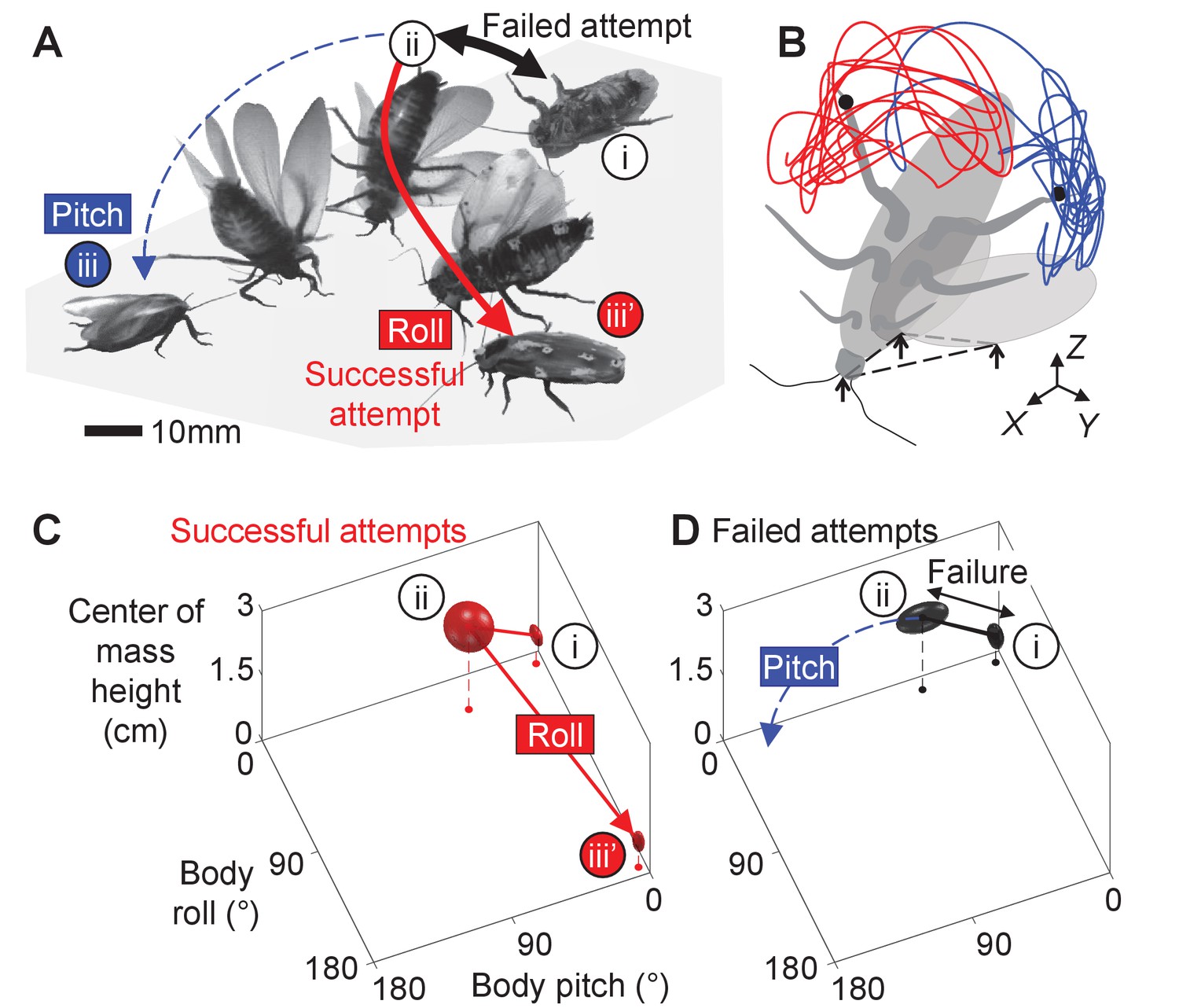
Strenuous, leg-assisted, winged ground self-righting of discoid cockroach.
(A) Representative snapshots of animal successfully self-righting by pitch (blue) and roll (red) modes after multiple failed attempts (black arrow). See Figure 1—video 1 for a typical trial, in which the animal makes multiple failed attempts to pitch over the head and eventually rolls to self-right. (B) Schematic of metastable state with a triangular base of support (dashed triangle) formed by ground contacts of head and two wing edges, with vigorous leg flailing. Red and blue curves show representative trajectories of left and right hind leg tips from a trial. X-Y-Z is lab frame. (C, D) Stereotyped body motion during successful (C) and failed (D) self-righting attempts in body pitch, body roll, and center of mass height space. i, ii, and iii in A, C, and D show upside-down (i), metastable (ii), and upright (iii, iii’) states, respectively. Ellipsoids show means (center of ellipsoid) ± s.d. (principal semi-axis lengths of ellipsoid) of body pitch, body roll, and center of mass height at the beginning, highest center of mass height, and end of the attempt. For failed attempts, the upside-down state at the end of the attempts is not shown because it overlaps with the upside-down state at the start of the attempts (i). Data from Li et al., 2019.
Figure 1—video 1
Strenuous leg-assisted, winged self-righting with multiple failed attempts.
A discoid cockroach makes multiple failed attempts to pitch over the head by opening and pushing its wings against the ground and eventually rolls to self-right.
Figure 1—video 2
A discoid cockroach using wing opening and leg flailing together during strenuous winged self-righting.
A discoid cockroach opening and pushing its wings against ground and flailing its legs to self-right from a metastable state. Blue and red curves show trajectories of left and right hind leg tips. Green arrows show ground contact points forming a triangular base of support.
Figure 2 with 2 supplements
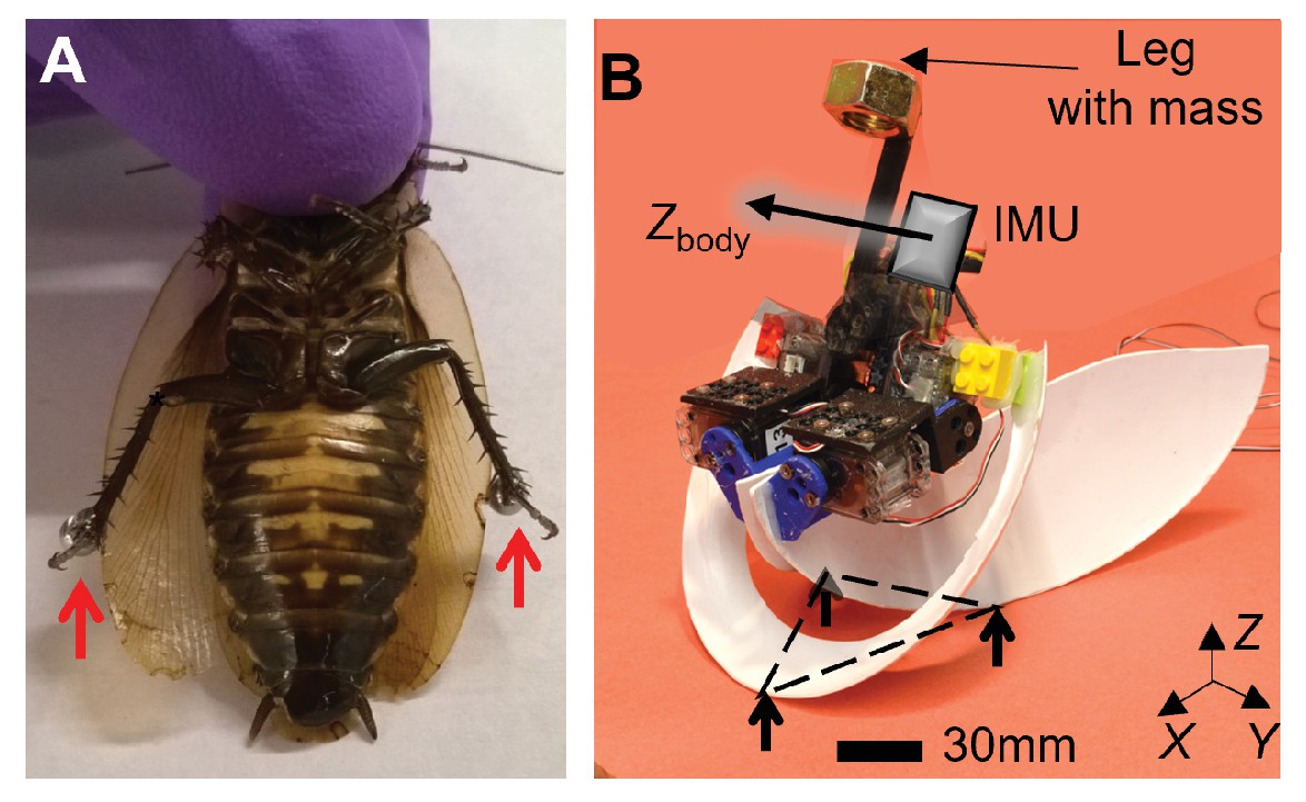
Animal leg modification and robotic physical model.
(A) Discoid cockroach with modified hind legs with stainless steel spheres attached. (B) Robotic physical model in metastable state with a triangular base of support (dashed triangle), formed by ground contacts of head and two wing edges. Black arrow shows body Z-axis, Zbody.
Figure 2—figure supplement 1

Robot wing and leg actuation and body orientation measurement.
(A) Schematic of leg-assisted, winged self-righting robot from front and side views with geometric dimensions. Front view illustrates wing rolling and leg oscillation and side view illustrates wing pitching. Wing pitching and rolling are by the same angle, synchronized, and together compose wing opening. (B) Motor angles of wings (blue) and leg (red) as a function of time. Solid and dashed curves are commanded and measured motor actuation profiles, respectively. (C) Projection of gravitational acceleration vector onto body Z-axis body as a function of time, measured using onboard inertial measurement unit (IMU). Vertical dashed line shows the instant when the robot self-righted. In B, C, columns i and ii are for a representative failed and successful trial, respectively.
Figure 2—video 1
Wing and leg actuation of robotic physical model.
Wings can both pitch and roll relative to body. Leg oscillation emulates leg flailing of animal (inset).
Figure 3 with 4 supplements
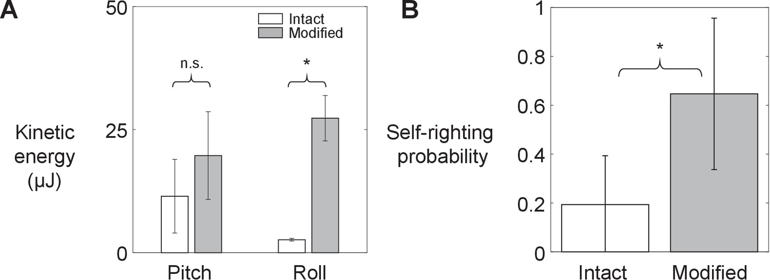
Animal’s kinetic energy and self-righting probability.
Comparison of (A) average pitch and roll kinetic energy and (B) self-righting probability between intact animals and animals with modified hind legs. Error bars show ± s.d. Asterisk indicates a significant difference (p < 0.05) and n.s. indicates none. Statistical tests: Pitch kinetic energy: p = 0.34, F1, 1 = 1.53, ANOVA. Roll kinetic energy: p = 0.02, F1, 1 = 50.35, ANOVA. Probability: p < 0.0001, F1, 29 = 93.38, mixed-effects ANOVA. Sample size: (A) N = 2 animals, n = 2 trials. (B) Intact: N = 30 animals, n = 150 trials. Modified: N = 30 animals, n = 150 trials.
Figure 3—figure supplement 1

Animal kinetic energy calculation.
(A) Representative snapshot of body and appendage with definition of markers tracked. (B) Multi-body model of animal for calculating pitch and roll kinetic energy. Red and blue arrows show velocity components that contribute to pitch and roll kinetic energy, respectively. (C) Pitch and roll kinetic energy as a function of time for animal with (i) intact and (ii) modified hind legs from a representative trial.
Figure 3—figure supplement 2
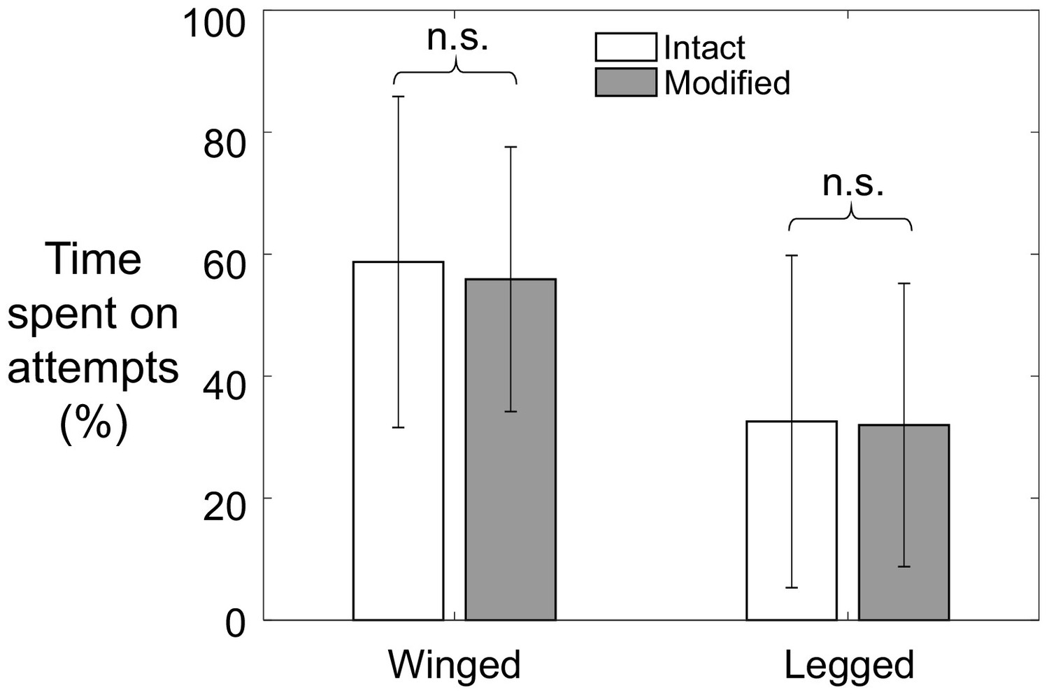
Comparison of average percentage of time spent on winged and legged self-righting attempts between animals with intact and modified legs.
Error bars show ± s.d. n.s. indicates no significant difference. Winged: p = 0.19, F1,269 = 1.71; legged: p = 0.78, F1,269 = 0.07 mixed-effects ANOVA. Sample size: N = 30 animals, n = 150 trials for each treatment.
Figure 3—figure supplement 3
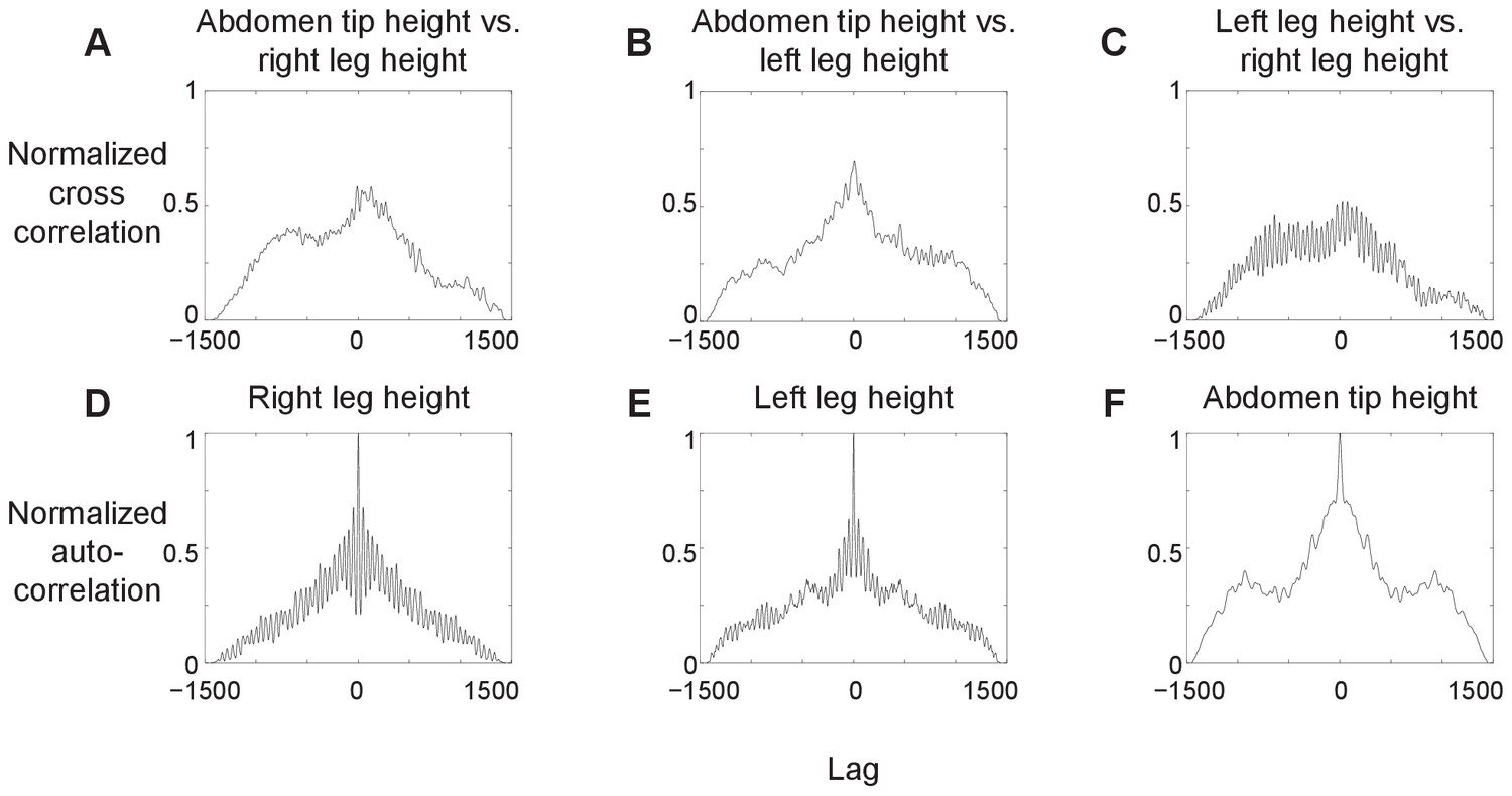
Correlation between animal’s body and leg motion.
(A–C) Pair-wise normalized cross-correlations between left hind leg tip height, right hind leg tip height, and abdomen tip height, as a function of lag between each pair of variables. (D–F) Normalized autocorrelation of left hind leg tip height, right hind leg tip height, and abdomen tip height as a function of lag between a variable and itself. N = 1 animal, n = 1 trial.
Figure 3—video 1
Leg flailing kinetic energy facilitates winged self-righting of animal.
Representative trials of strenuous leg-assisted, winged self-righting with and without hind leg modification (played three times).
Figure 4 with 1 supplement

Robot’s kinetic energy and self-righting performance.
(A, B) Average pitch and roll kinetic energy during self-righting as a function of leg oscillation amplitude θleg at different wing opening amplitudes θwing. (C, D) Self-righting probability and average number of attempts required to self-right as a function of θleg at different θwing. Error bars in A, B, and D are ± s.d., and those in C are confidence intervals of 95%. Asterisks indicate a significant dependence (p < 0.05) on θleg at a given θwing and n.s. indicates none. See Figure 4—source data 1 for details of statistical tests. Sample size: Kinetic energy: n = 20 attempts at each wing opening amplitude. Self-righting probability and number of attempts: n = 58, 42, and 34 attempts at θwing = 60°, 72°, and 83°. For kinetic energy, only the first attempt from each trial is used to measure the average to avoid bias from large pitching or rolling motion during subsequent attempts that self-right.
-
Figure 4—source data 1
Statistical test results for Figure 4A–D.
- https://cdn.elifesciences.org/articles/60233/elife-60233-fig4-data1-v2.xlsx
Figure 4—video 1
Wing opening and leg flailing together facilitate winged self-righting of robot.
Left: Representative videos from top and front views. Top right: Commanded (solid) and measured (dashed) motor angles as a function of time. Blue and red curves are for wing and leg motors, respectively. Bottom right: Projection of gravitational acceleration vector on body Z-axis as a function of time, measured by onboard inertial measurement unit (IMU). Video first shows a failed trial without leg oscillation and then a successful trial with leg oscillation.
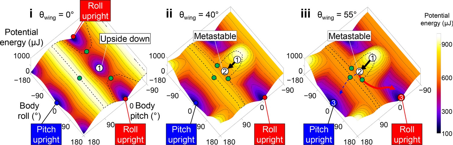
Figure 5 with 4 supplements

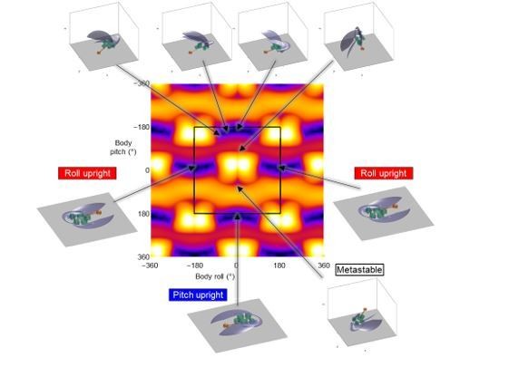
Robot’s self-righting motion and potential energy landscape.
(A) Snapshots of reconstructed robot upside-down (i), in metastable state (ii), self-righting by pitch (iii) and roll (iii’) modes, and upright afterward (iv, iv’). (B) Snapshots of potential energy landscape at different wing opening angles corresponding to (A) i, ii, iii. Dashed curves are boundary of upside-down/metastable basin. Green dots show saddles between metastable basin and the three upright basins. Gray curves show constant potential energy contours. Black, dashed blue, and red curves are representative trajectories of being attracted to and trapped in metastable basin, self-righting by pitch mode, and self-righting by roll mode, respectively. i, ii, iii in (A, B) show upside-down (1), metastable (2), and upright (3iii, iii’) states, respectively. (C) Polar plot of potential energy barrier to escape from upside-down or metastable local minimum along all directions in pitch-roll space. ψ is polar angle defining direction of escape in body pitch-roll space. Green arrow in (i) shows direction of upright minima at pitch = 180° (ψ = 0°). Black circle shows scale of energy barrier (100 mJ). Blue and red arrows in (ii) define pitch and roll potential energy barriers. Blue and red error bars in (iii) show average maximal pitch and roll kinetic energy, respectively.
Figure 5—figure supplement 1
Animal’s potential energy landscape.
Snapshots of potential energy landscape at different wing opening angles. Black curve is representative trajectories of failed attempts and dashed blue and red curves are for successful attempt by pitch mode and self-righting by roll mode, respectively. Thin black curves on landscape are constant potential energy contours. Dashed black curves show boundary of upside-down/metastable basins. Green dots show saddles between metastable basin and the three upright basins.
Figure 5—video 1
Robot potential energy landscape modeling.
Top left: Illustrative robot body motion for self-righting via pitch and roll modes. Top right: Evolution of potential energy landscape as wings open, with robot state (dot) and state trajectory. Black curve is for robot opening its wings and becoming trapped in metastable basin. Blue dashed and red solid curves are for robot escaping metastable basin via pitch and roll modes, respectively. Bottom right: Potential energy barrier to escape from upside-down or metastable local minimum along all directions in body pitch-roll space. Green arrow shows direction of pitch upright minima at pitch = 180°. Blue and red error bars show pitch and roll kinetic energy, respectively. Bottom left: Pitch (blue) and roll (red) barrier as a function of wing opening angle. Blue and red dashed lines show pitch and roll kinetic energy, respectively. Gray band shows range of wing opening amplitudes tested.
Figure 5—video 2
Robot state trajectory on potential energy landscape.
Top left: Representative trial. Bottom left: Reconstructed 3D motion. Right: Potential energy landscape with robot state (dot) and state trajectory. Video first shows a failed trial without leg oscillation and then a successful trial with leg oscillation. Note that only the end point of the trajectory, which represented the current state, showed the actual potential energy of the system at the corresponding wing opening angle. The rest of the visualized trajectory showed how body pitch and roll evolved but, for visualization purpose, was simply projected on the landscape surface.
Figure 5—video 3
Bifurcation diagram for animal’s potential energy landscape.
Top left: Potential energy landscape over body pitch-roll space and its equilibrium points along body roll = 0° (blue dots) and body pitch = 0° (red dots). Top right: Body pitch of equilibrium points along body roll = 0° (blue dots) as a function of wing opening angle. Bottom left: Body roll of equilibrium points along body pitch = 0° (red dots) as a function of wing opening angle. Solid and dashed lines show stable and unstable equilibria, respectively. * shows saddle-node bifurcations where a stable equilibrium and an unstable one merge. Only the points that are an equilibrium along both roll and pitch directions are shown.
Figure 6 with 2 supplements
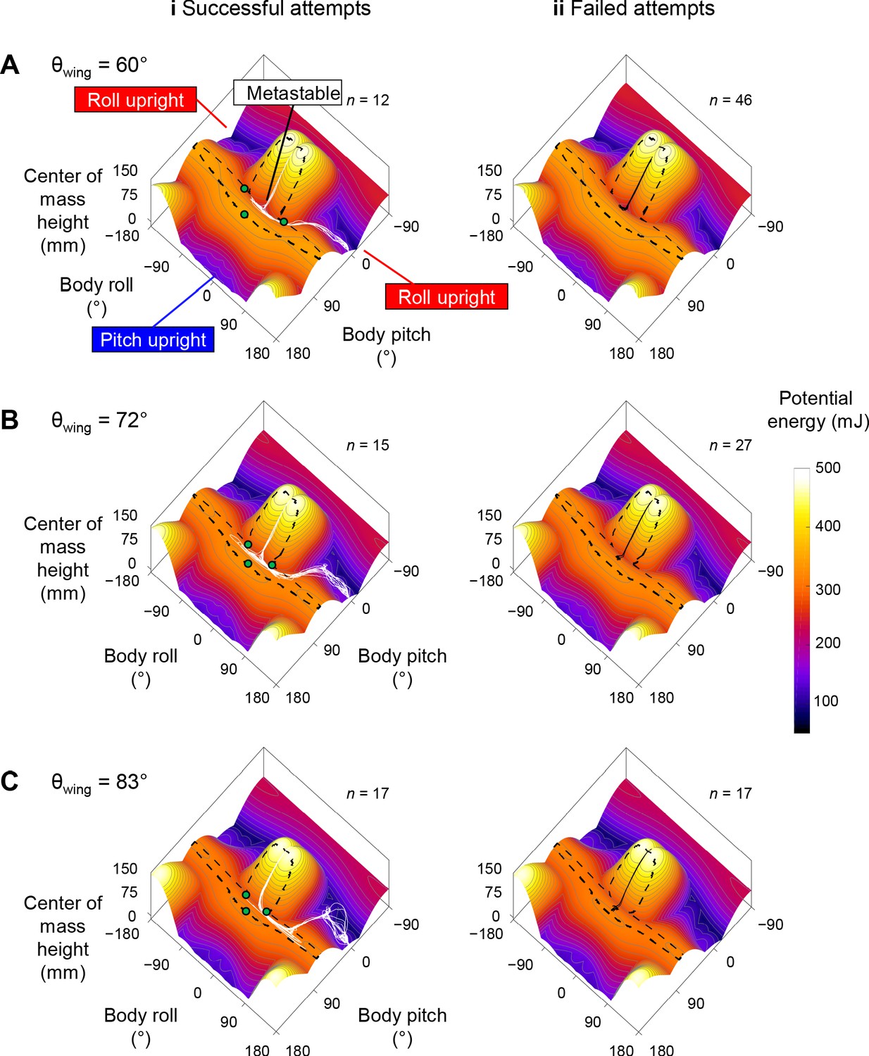
Robot state trajectories on potential energy landscape.
(A) θwing = 60°. (B) θwing = 72°. (C) θwing = 83°. Columns i and ii show successful (white) and failed (black) self-righting attempts, respectively. n is the number of successful or failed attempts at each θwing. Note that only the end point of the trajectory, which represented the current state, showed the actual potential energy of the system at the corresponding wing opening angle. The rest of the visualized trajectory showed how body pitch and roll evolved but, for visualization purpose, was simply projected on the landscape surface. Gray lines show energy contours. Green dots show saddles between metastable basin and the three upright basins.
Figure 6—figure supplement 1
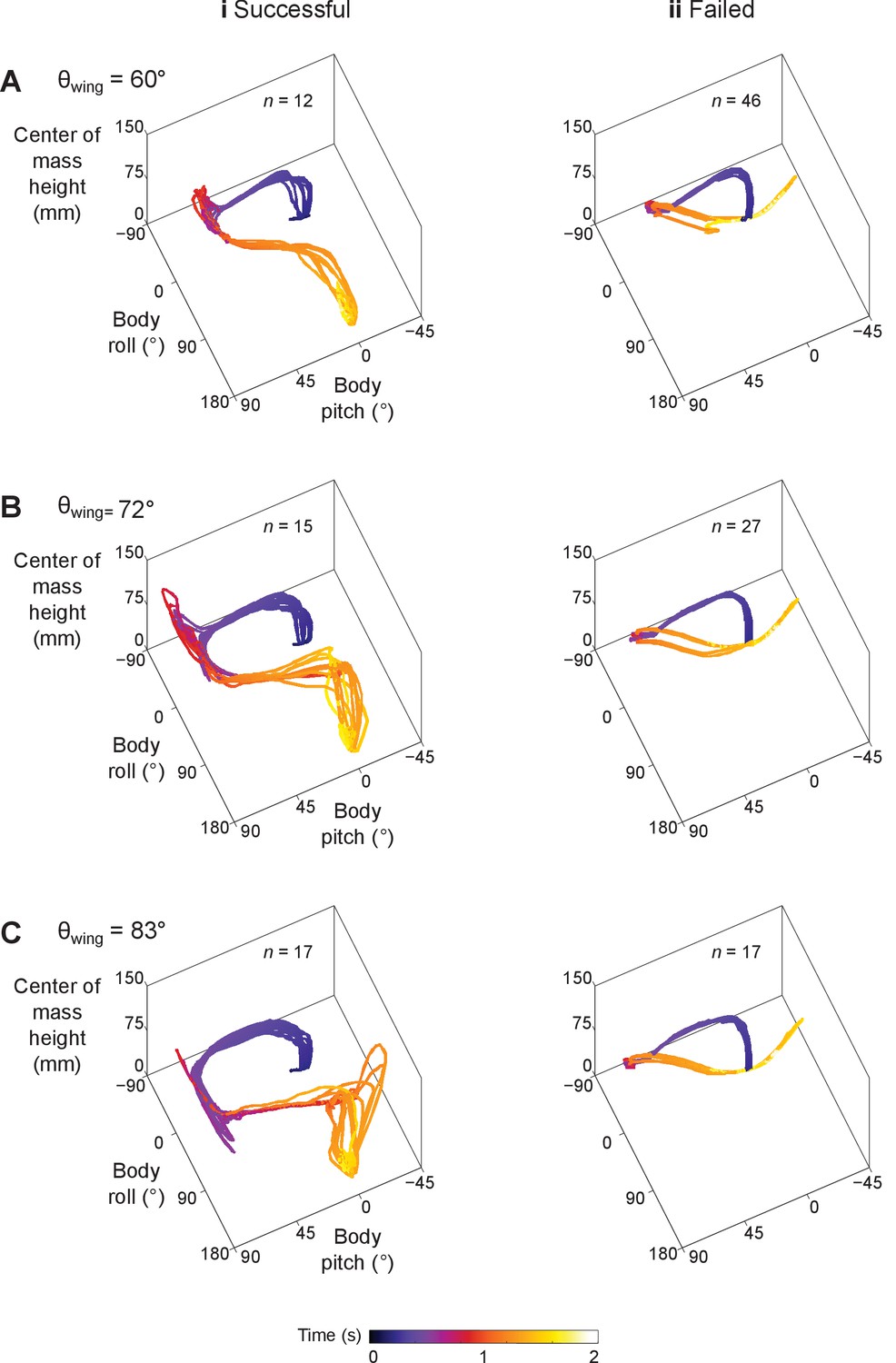
Robot’s stereotyped body motion during self-righting.
State trajectories in body pitch, body roll, and center of mass height space. (A) θwing = 60°. (B) θwing = 72°. (C) θwing = 83°. Columns i and ii show successful and failed self-righting attempts, respectively. n is the number of successful or failed attempts at each θwing.
Figure 6—video 1
Robot state trajectory ensemble on potential energy landscape.
Evolution of potential energy landscape and robot state trajectories during self-righting attempts. White and black curves show trajectories for successful and failed self-righting attempts, respectively. Green and pink dots show system state for successful and failed attempts, respectively. Note that only the end point of the trajectory, which represented the current state, showed the actual potential energy of the system at the corresponding wing opening angle. The rest of the visualized trajectory showed how body pitch and roll evolved but, for visualization purpose, was simply projected on the landscape surface.
Figure 7 with 3 supplements
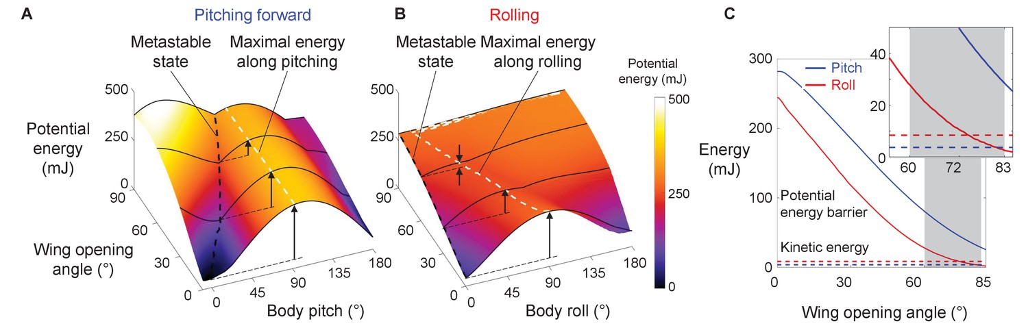
Robot’s potential energy barriers for self-righting via pitch and roll modes.
(A) Potential energy during self-righting via pitch mode as a function of body pitch and wing opening angle. (B) Potential energy during self-righting via roll mode as a function of body roll and wing opening angle. Dashed black curves in A and B show energy of metastable state. Dashed white curves in A and B shows maximal energy when pitching forward or rolling from metastable state, respectively. Vertical upward arrows define pitch (A) and roll (B) barriers at a few representative wing opening angles. (C) Pitch (blue) and roll (red) barrier as a function of wing opening angle. Blue and red dashed lines show average maximal pitch and roll kinetic energy, respectively. Gray band shows range of wing opening amplitudes tested. Inset shows the same data magnified to better show kinetic energy.
-
Figure 7—source data 1
Statistical test results for Figure 7—figure supplements 2 and 3.
n = 134 attempts.
- https://cdn.elifesciences.org/articles/60233/elife-60233-fig7-data1-v2.xlsx
Figure 7—figure supplement 1
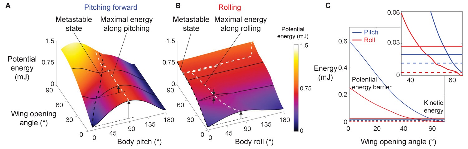
Animal’s potential energy barriers for self-righting via pitch and roll modes.
(A) Potential energy of self-righting via pitch mode as a function body pitch and wing opening amplitude. (B) Potential energy of self-righting via roll mode as a function of body roll and wing opening amplitude. Dashed black curves in A and B show energy of metastable state. Dashed white curves in A and B shows maximal energy when pitching forward or rolling from metastable state, respectively. Vertical arrows define pitch (A) and roll (B) barriers at a few representative wing opening angles. (C) Pitch (blue) and roll (red) barrier as a function of wing opening angle. Dashed and solid horizontal lines show the intact (dashed) and modified (solid) animal’s average pitch kinetic energy (blue) and average roll kinetic energy (red), respectively. Inset shows the same data magnified to better show kinetic energy.
Figure 7—figure supplement 2
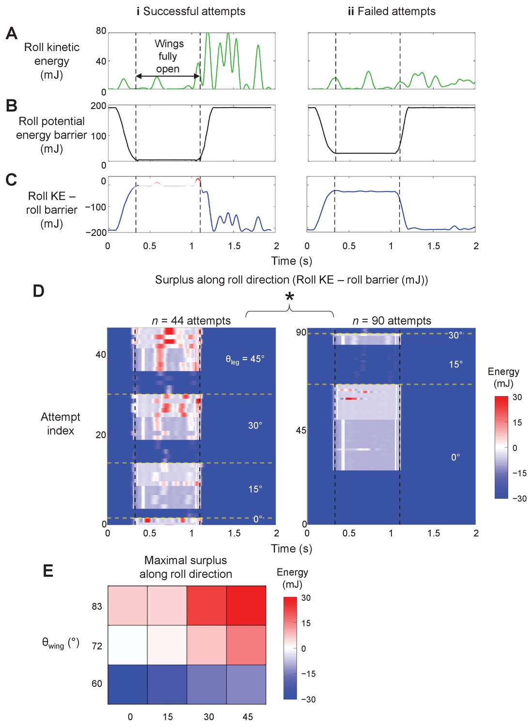
Comparison between robot’s roll kinetic energy and roll potential energy barrier.
(A) Roll kinetic energy, (B) roll potential energy barrier, and (C) roll kinetic energy minus potential energy barrier along roll direction over time for a representative successful and failed attempt. Between two vertical dashed lines is when wings are held fully open. (D) Surplus along roll direction over time for all attempts from all trials. The attempts are grouped along vertical axis, based on increasing leg oscillation amplitude θleg. For each θleg, the attempts are further grouped along by different wing opening amplitudes θwing (increasing along upward direction). Columns (i) and (ii) are successful and failed attempts, respectively. Asterisk indicates significant difference in roll kinetic energy minus potential energy barrier between successful and failed attempts. (E) Average of maximal roll kinetic energy minus potential energy barrier, as a function of wing opening amplitude and leg oscillation amplitude. Red and blue show surplus and deficit of roll kinetic energy minus potential energy barrier, respectively. n = 134 attempts. See Figure 7—source data 1 for results of statistical tests.
Figure 7—figure supplement 3

Comparison between robot’s pitch kinetic energy and pitch potential energy barrier.
(A) Kinetic energy, (B) potential energy barrier, and (C) kinetic energy minus potential energy barrier as a function of time for a representative successful (i) and failed (ii) attempt. Between two vertical dashed lines is when wings are held fully open. (D) Pitch kinetic energy minus potential energy barrier as a function of time of all attempts from all trials. Along vertical axis, attempts are grouped into increasing leg oscillation amplitude θleg. For each θleg, attempts are further grouped into increasing wing opening amplitudes θwing. Columns (i) and (ii) are successful and failed attempts, respectively. Asterisk indicates significant difference in pitch kinetic energy minus potential energy barrier between successful and failed attempts. (E) Average of maximal pitch kinetic energy minus potential energy barrier when wings are fully open as a function of θwing and θleg. Red and blue show surplus and deficit of pitch kinetic energy minus potential energy barrier, respectively. n = 134 attempts. See Figure 7—source data 1 for results of statistical tests.
Figure 8 with 1 supplement
Dependence of potential energy landscape on ground geometry.
(A) Grounds of different geometry. (i) Flat ground. (ii, iii) Uneven ground with small (ii) and large (iii) asperities compared to animal/robot size. (B) Potential energy landscapes for self-righting on corresponding ground. In ii and iii, landscape is not invariant to robot body translation as in i. Landscape is shown for robot at the geometric center of the terrain with wings closed. Robot shown for scale.
Figure 8—video 1
Potential energy landscape changes with ground geometry.
Potential energy landscape evolves as wing opening angle increases. Definitions follow Figure 8.
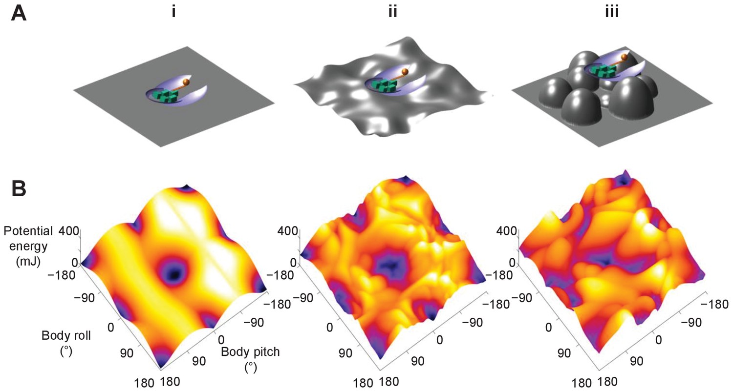
Author response image 1
Potential energy landscape for an extended body pitch-roll space.
Landscape shown for a wing opening angle of 51.2°. Black square shows the range of landscape used in the paper for analysis. Panels show the statically stable equilibrium configurations of the robot. Black arrows point to body pitch and roll corresponding to stable orientations.
Tables
Table 1
Mass distribution of the robot.
| Component | Mass (g) |
|---|---|
| Head | 13.4 |
| Leg rod | 4.3 |
| Leg added mass | 51.5 |
| Leg motor | 28.6 |
| Two wings | 57.4 |
| Two wing pitch motors | 56.0 |
| Two wing roll motors | 48.8 |
| Total | 260.0 |
Table 2
Comparison between animal and robot.
| Parameter | Animal | Robot | Ratio | |
|---|---|---|---|---|
| Body length 2a (mm) | 53 | 260 | 4.9 | |
| Body width 2b (mm) | 23 | 220 | 9.6 | |
| Body thickness 2c (mm) | 8 | 43 | 5.4 | |
| Mass attached to leg (g) | 0.14 | 51.5 | 368 | |
| Total mass m* (g) | 2.84 | 260 | 90 | |
| Density ρ (×10−3 g mm−3) | 0.88 | 2.05 | 2.3 | |
| Expected length scale factor (m/ρ)1/3 | 1.47 | 5.06 | 3.4 | |
| Expected potential energy scale factor m4/3/ρ1/3 | 4.28 | 1306 | 305 | |
| Maximum pitch potential energy barrier (mJ) | 0.58 | 282 | 486 | |
| Maximum roll potential energy barrier (mJ) | 0.19 | 244 | 1284 | |
| Froude number for leg flailing Fr | Intact legs | 0.37 | 0.78 | 2.1 |
| Modified legs | 1.27 | 0.61 | ||
-
*Includes mass attached to the legs.
Additional files
Download links
A two-part list of links to download the article, or parts of the article, in various formats.
Downloads (link to download the article as PDF)
Open citations (links to open the citations from this article in various online reference manager services)
Cite this article (links to download the citations from this article in formats compatible with various reference manager tools)
Propelling and perturbing appendages together facilitate strenuous ground self-righting
eLife 10:e60233.
https://doi.org/10.7554/eLife.60233


