Exploring chromosomal structural heterogeneity across multiple cell lines
- Center for Theoretical Biological Physics, Rice University, United States
- Brazilian Biorenewables National Laboratory - LNBR, Brazilian Center for Research in Energy and Materials - CNPEM, Brazil
- Center for Genome Architecture, Baylor College of Medicine, United States
- Department of Chemistry, Rice University, United States
- Department of Physics & Astronomy, Rice University, United States
- Department of Biosciences, Rice University, United States
- Department of Physics, Northeastern University, United States
Figures
Figure 1 with 5 supplements
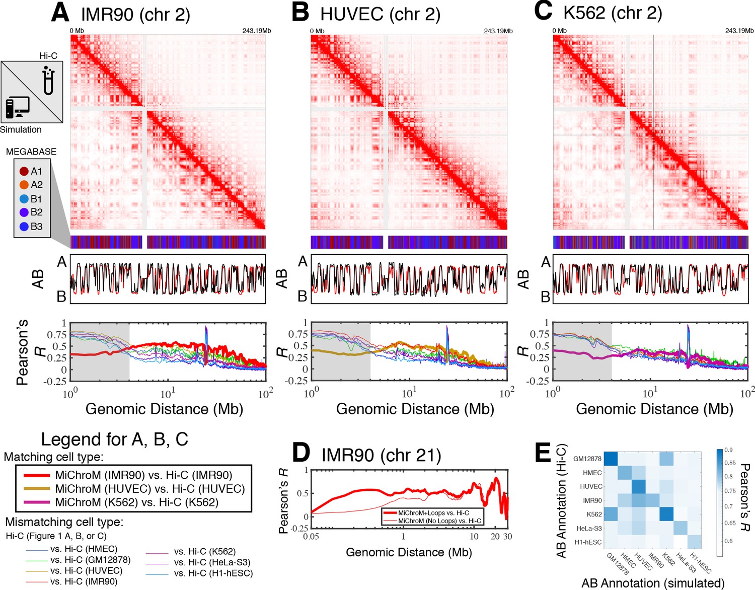
Prediction of chromosome structures for differentiated cell lines and for immortalized leukemia cells.
The 3D ensemble of chromosome structures was predicted for the cell types (A) IMR90, (B) HUVEC, and (C) K562 using the ChIP-Seq histone modification tracks for the respective cell lines found on ENCODE—shown are the structural predictions for chromosome 2. As validation, the chromosome structures were compared with the DNA–DNA ligation experiments of Rao et al., 2014, where the simulated map is shown on the bottom left triangle and the experimental map is shown on the top right triangle. The datasets are visualized using Juicebox (Durand et al., 2016). The MEGABASE chromatin type annotation is shown as a color vector under the contact probability map, followed by the A/B compartment annotation (Rao et al., 2014) for the simulated map (red) and the experimental map (black), respectively. The Pearson’s R between the simulated and experimental contact maps for fixed genomic distances are plotted for the cell types IMR90, HUVEC, and K562, respectively, in thick lines. The Pearson’s R between the experimental maps of mismatching cell types are also shown with thin lines—See Legend. The shaded region highlights that at relatively short genomic distances (<10 Mb), excluding CTCF-mediated loops from the simulation results in disagreement between the simulated and experimental maps. When loops are included in the simulations, the agreement between the simulation and experiment is recovered at the short genomic distances. (D) Pearson’s R as a function of genomic distance is plotted between the experimental map for chromosome 21 (IMR90) and MiChroM simulation with loops (thick red line) and without loops (thin red line). (E) A matrix of Pearson’s R between the AB annotation of the experimental ligation map and the simulated contact maps for different cell types, respectively. The high Pearson’s R signifies the consistency between the simulated maps and the experimental DNA–DNA ligation maps. Additional comparisons between simulated and experimental DNA–DNA ligation maps are shown for cell lines HMEC, H1-hESC, and HeLa-S3 in Figure 1—figure supplements 1–3, respectively. A matrix of Pearson’s R between the AB annotation of the experimental ligation maps for different cell types is shown in Figure 1—figure supplement 4.
Figure 1—figure supplement 1
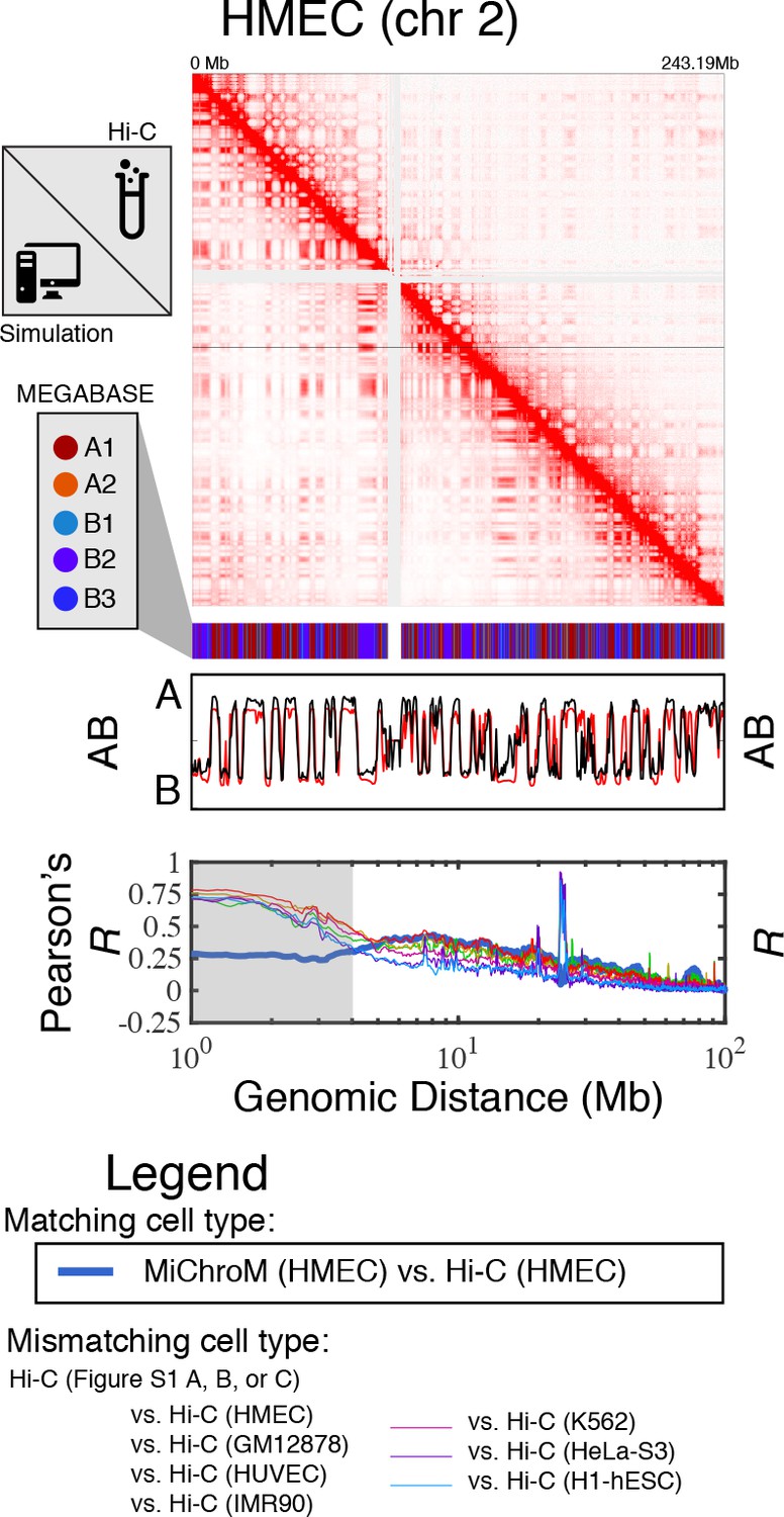
Prediction of chromosome structures for HMEC.
The 3D ensemble of chromosome structures was predicted for the HMEC cell type using the ChIP-Seq histone modification tracks found on ENCODE—shown are the structural predictions for chromosome 2. As validation, the chromosome structures were compared with the DNA–DNA ligation experiments of Rao et al., 2014, where the simulated map is shown on the bottom left triangle and the experimental map is shown on the top right triangle. The datasets are visualized using Juicebox (Durand et al., 2016). The MEGABASE chromatin type annotation is shown as a color vector under the contact probability map, followed by the A/B compartment annotation (Rao et al., 2014) for the simulated map (red) and the experimental map (black), respectively. The Pearson’s R between the simulated and experimental contact maps for fixed genomic distances are plotted for HMEC with a thick line. The Pearson’s R between the experimental maps of mismatching cell types are also shown with thin lines—See Legend.
Figure 1—figure supplement 2
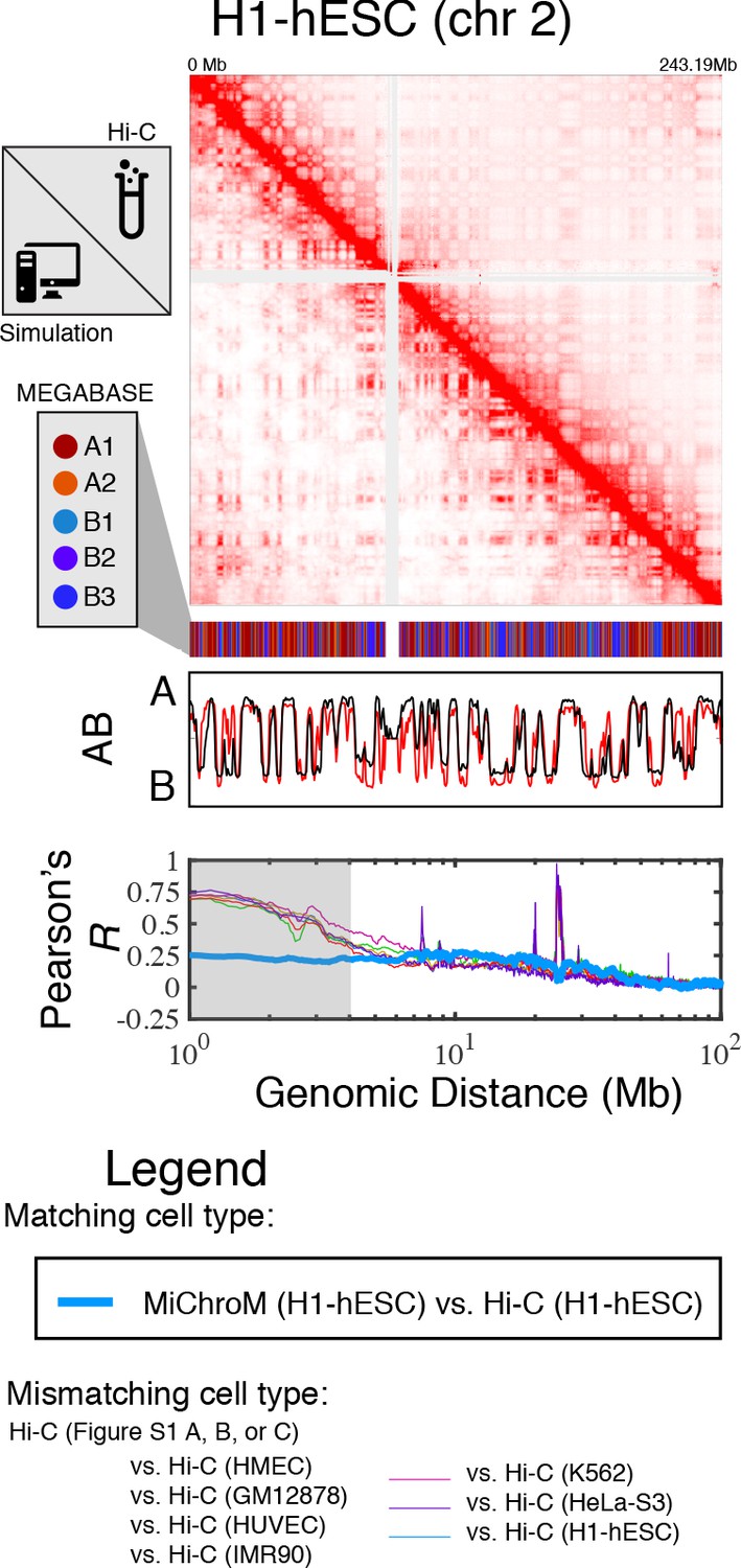
Prediction of chromosome structures for H1-hESC.
The 3D ensemble of chromosome structures was predicted for the H1-hESC cell type using the ChIP-Seq histone modification tracks found on ENCODE—shown are the structural predictions for chromosome 2. As validation, the chromosome structures were compared with the DNA–DNA ligation experiments of Dixon et al., 2012, where the simulated map is shown on the bottom left triangle and the experimental map is shown on the top right triangle. The datasets are visualized using Juicebox (Durand et al., 2016). The MEGABASE chromatin type annotation is shown as a color vector under the contact probability map, followed by the A/B compartment annotation for the simulated map (red) and the experimental map (black), respectively. The Pearson’s R between the simulated and experimental contact maps for fixed genomic distances are plotted for H1-hESC with a thick line. The Pearson’s R between the experimental maps of mismatching cell types are also shown with thin lines—See Legend.
Figure 1—figure supplement 3
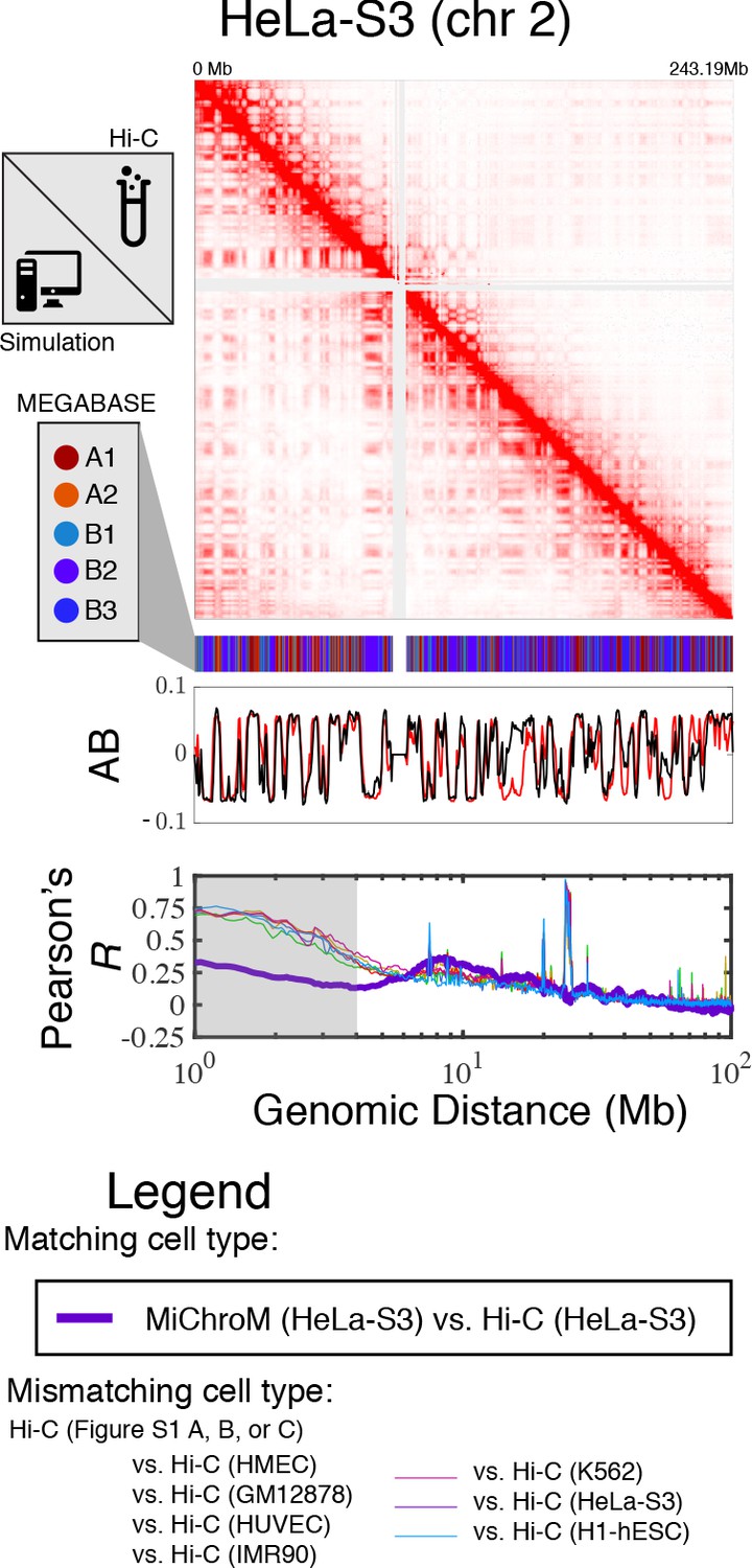
Prediction of chromosome structures for HeLa-S3.
The 3D ensemble of chromosome structures was predicted for the HeLa-S3 cell type using the ChIP-Seq histone modification tracks found on ENCODE—shown are the structural predictions for chromosome 2. As validation, the chromosome structures were compared with the DNA–DNA ligation experiments of Rao et al., 2014, where the simulated map is shown on the bottom left triangle and the experimental map is shown on the top right triangle. The datasets are visualized using Juicebox (Durand et al., 2016). The MEGABASE chromatin type annotation is shown as a color vector under the contact probability map, followed by the A/B compartment annotation (Rao et al., 2014) for the simulated map (red) and the experimental map (black), respectively. The Pearson’s R between the simulated and experimental contact maps for fixed genomic distances are plotted for HeLa-S3 with a thick line. The Pearson’s R between the experimental maps of mismatching cell types are also shown with thin lines—See Legend.
Figure 1—figure supplement 4
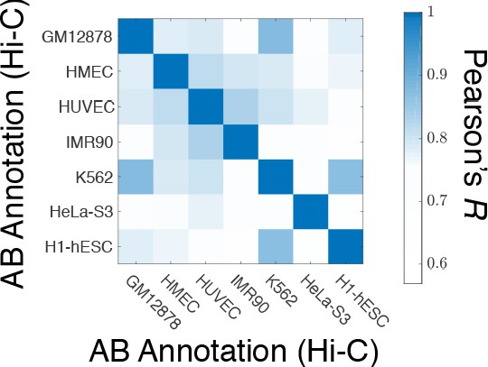
A matrix of Pearson’s R between the AB annotation of the experimental ligation maps for different cell types.
The diagonal elements of this matrix show the Pearson’s R of a particular AB annotation from Hi-C with itself and is equal to one by definition.
Figure 1—figure supplement 5
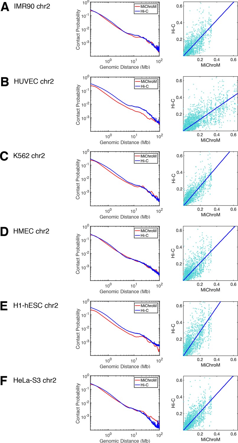
Comparison of the experimental and simulated DNA–DNA ligation maps: power law scaling and scatter plot.
For each cell type (A–F), the power law scaling of the contact probability as a function of genomic distance is shown in the left panel, while the right-most panel shows the scatter plot of the contact probabilities of the experimental and simulated maps. The slope and intercept of the scatter plots: (A) IMR90: 1.0725, 0.0001 (B) HUVEC: 0.6865, 0.0006, (C) K562: 1.1695,–0.0001, (D) HMEC: 1.0479,–0.0001, (E) H1-hESC: 1.4557, 0.0001, (F) HeLa-S3: 1.0926,–0.0003. The average contact probability from experiment for HUVEC (B) and H1-hESC (E) are notably higher than those from simulation, suggesting that the chromosome densities in those corresponding simulations are lower than in experiment. All of our chromosome simulations are performed with a volume fraction of chromatin in the interphase of 0.1 (Rosa and Everaers, 2008).
Figure 2 with 4 supplements
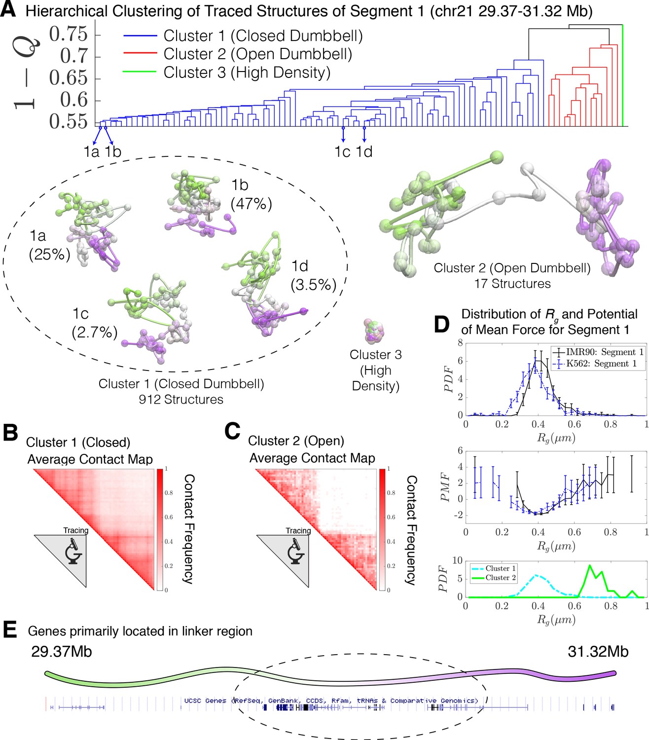
Hierarchical clustering and the detailed structural analysis of traced Segment 1.
(A) The dendrogram representation of the hierarchical clustering of Segment 1 (chr21 29.37–31.32 Mb for IMR90 and K562 of Bintu et al., 2018), where is used as the distance between two structures. The clustering reveals three main clusters: closed dumbbell, open dumbbell, and highly dense structures. Further analysis of Cluster 1 reveals the presence of sub-clusters labeled 1a–1d that represent the gradual opening of the closed dumbbell. Representative traced structures are shown for each of the clusters and sub-clusters. The population-averaged contact maps for the closed and open structure clusters are shown respectively in (B) and (C), where 330 nm is used to define a contact between two 30 kb loci. (D) The distribution of the radius of gyration (top), the corresponding potential of mean force (center), and the distributions of radius of gyration for Cluster 1 and Cluster 2 (bottom) are shown for the traced structures of Segment 1 of IMR90 and K562. The distribution exhibits a heavy tail to the right of the average value, indicating the existence of open, elongated structures. (E) The UCSC Genes track is plotted along the genomic positions of Segment 1 using the Genome Browser (Kent et al., 2002). Figure 2—figure supplement 1 shows the contact maps for the experimentally traced segments of chromatin. Figure 2—figure supplement 2 shows the distributions of the radius of gyration for the sub-clusters of closed dumbbell structures obtained experimentally using tracing. Figure 2—figure supplement 3 shows the hierarchical clustering and detailed structural analysis of the experimentally traced Segment 2.
Figure 2—figure supplement 1
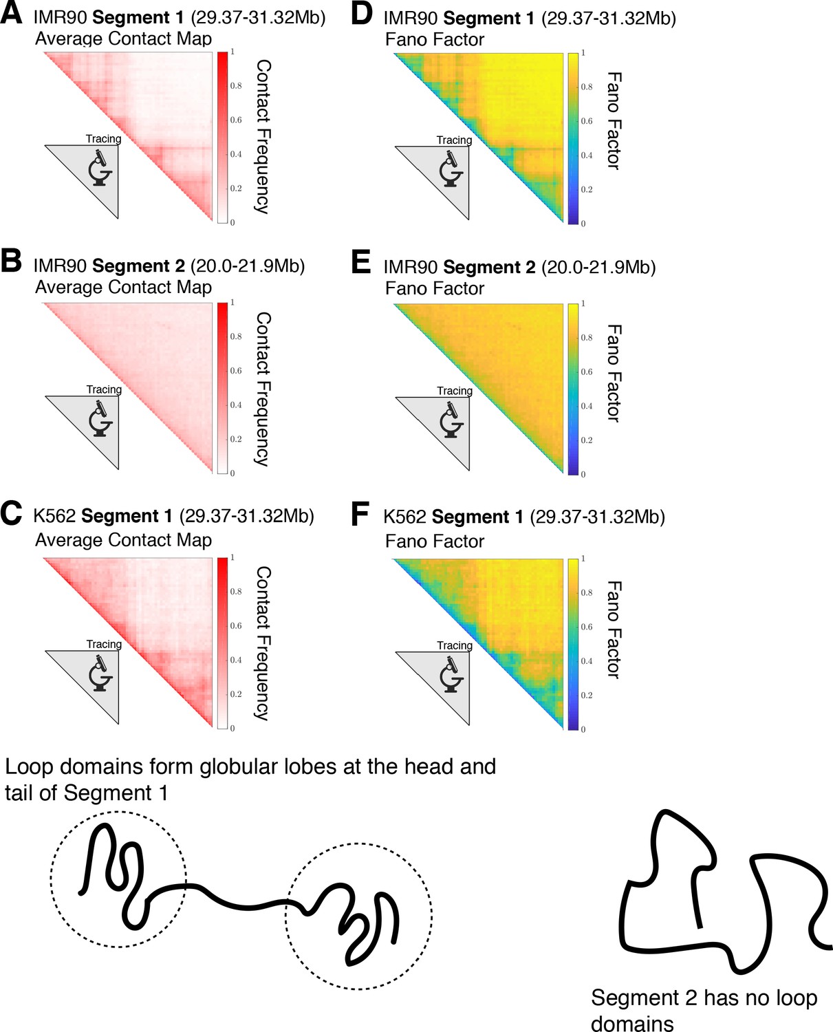
Contact maps for the experimentally traced segments of chromatin.
The contact maps for the chromatin structures obtained from super-resolution imaging (Bintu et al., 2018) for (A) IMR90 Segment 1 (chr 21 29.37–31.32 Mb), (B) IMR90 Segment 2 (chr 21 20.0–21.9 Mb), and (C) K562 Segment 1 (chr 21 29.37–31.32 Mb) are shown. For a given chromatin structure, two loci i and j are spatially proximal when the cartesian distance between them, , is less than or equal to a cutoff distance d—we define a contact using . This allows us to define a label for a pair of loci that equals one when loci i and j are in contact and 0 when they are not: . The variance of the contact frequency over the mean contact frequency (Fano Factor) is plotted for each of the respective chromatin segments in (D), (E), and (F), where the angular brackets denote averaging over the structural ensemble. A Fano factor of indicates zero variability, indicates that the process is under-dispersed and characterized by a binomial distribution, and is characteristic of a Poisson process. Segment 1 for IMR90 and K562 both have globular domains at the head and tail of the chromatin segment. On the other hand, Segment 2 has no loop domains and the only observable feature in its contact map is the decay of the contact probability as a function of genomic distance.
Figure 2—figure supplement 2
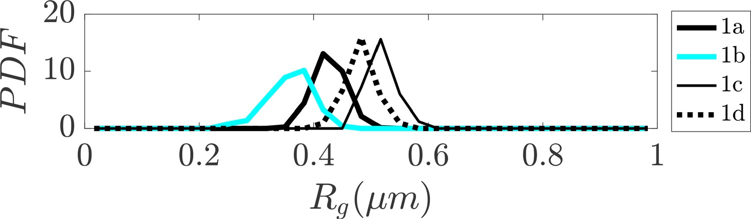
Distribution of radius of gyration for sub-clusters of closed dumbbell structures obtained experimentally using tracing.
Sub-clusters of Cluster one in Figure 2 are denoted as 1a, 1b, 1 c, and 1d. The sub-clusters of Cluster one characterize the gradual opening of the closed dumbbell structures.
Figure 2—figure supplement 3
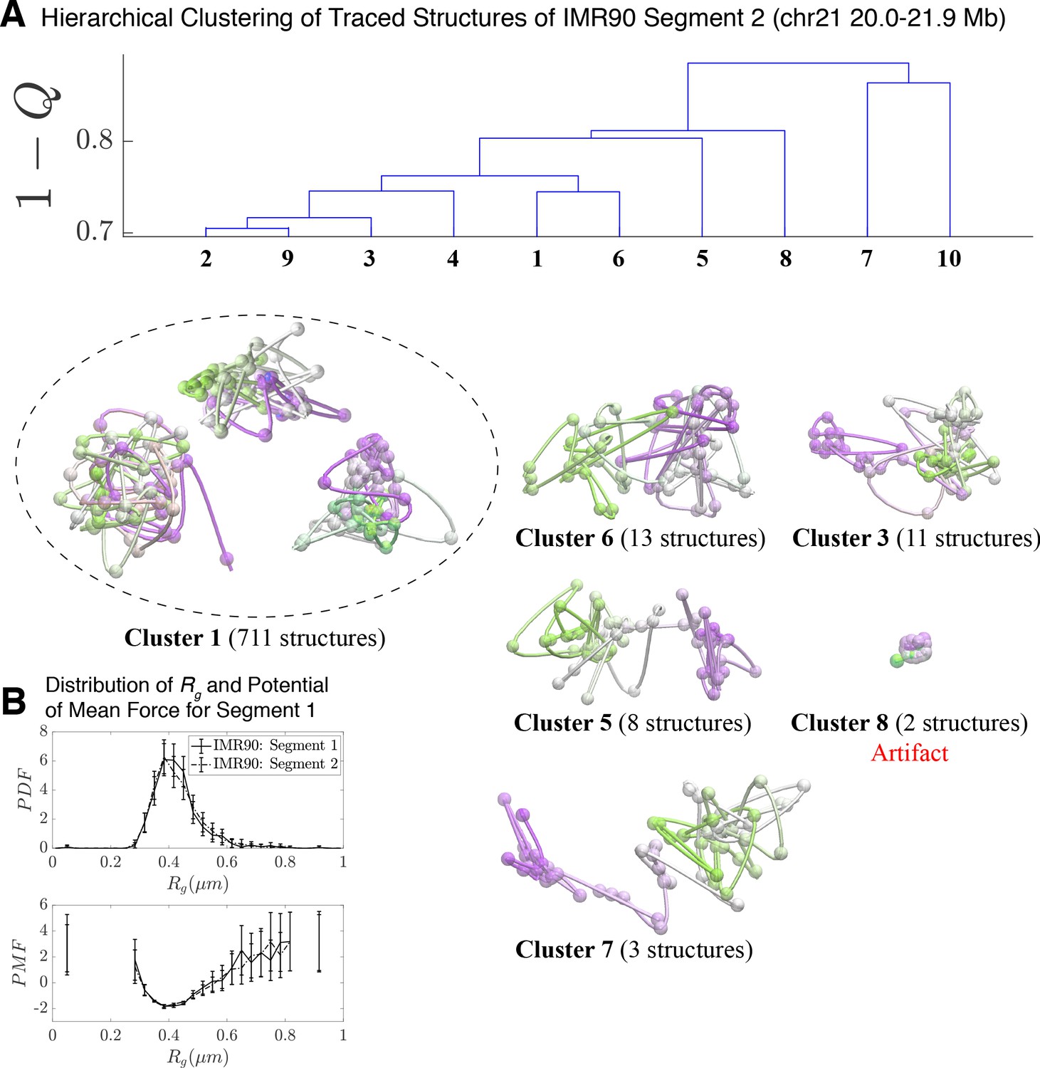
Hierarchical Clustering and the detailed structural analysis of traced Segment 2.
(A) The dendrogram representation of the hierarchical clustering of Segment 2 (chr 21 20.0–21.9 Mb for IMR90 of Bintu et al., 2018), where is used as the distance between two structures. The dendrogram highlights 10 clusters—representative structures are shown for each of the featured clusters. Cluster 1 bears a close relation to the closed dumbbell structures observed for Segment 1 (Figure 2). Cluster 8 captures the highly dense chromatin structures that are attributed to experimental artifact; analogous to Cluster three in Figure 2. The additional clusters capture the gradual opening of Segment 2. However, a striking difference from the structures of Segment 1 occurs due to the lack of loop domains in Segment 2; as a result, the globular domains at the head and tail of the segment observed for Segment 1 do not exist. The lack of loop domains and domain boundaries leads to disordered structures that deviate from the open dumbbell structures observed for Segment 1. (B) The distribution of the radius of gyration (top) and the corresponding potential of mean force (bottom) are shown for the traced structures of Segment 1 and Segment 2 of IMR90. Both distributions exhibit a heavy tail to the right of the average value, indicating the existence of open, elongated structures.
Figure 2—figure supplement 4
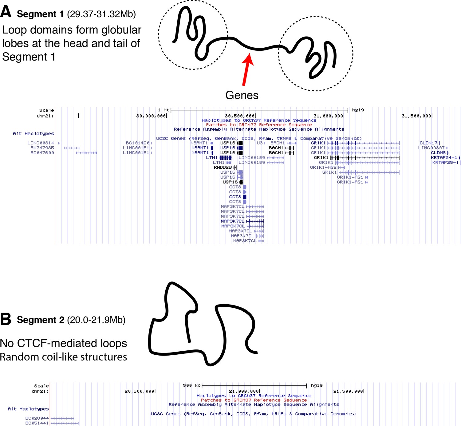
The positioning of genes along traced Segment 1 and Segment 2.
The UCSC Genome Browser (Kent et al., 2002) is used to plot the UCSC Gene Track for (A) traced Segment 1 and (B) traced Segment 2. The positioning of the genes along Segment 1 appears primarily in the linker region sandwiched between the globular domains that are at the head and tail of the chromatin segment. Segment 2, which has no loop domains, also coincidentally has an apparent absence of genes.
Figure 3 with 3 supplements

Hierarchical Clustering and the detailed structural analysis of simulated chromatin segment.
(A) The dendrogram representation of the hierarchical clustering of simulated Segment 1 (chr21 29.37–31.32 Mb for IMR90 and K562) where (Equation 1) is used as the distance between two structures. The clustering reveals two main clusters: closed dumbbell (6275 out of 6400 structures) and open dumbbell (125 out of 6400 structures). The closed dumbbell can be subdivided into sub-clusters labeled 1α−1δ that represent the opening transition of the closed dumbbell. Representative structures are shown for each of the clusters and sub-clusters. The population-averaged contact maps for the clusters are shown respectively in (B) and (C), where 330 nm is used to define a contact between two 50 kb loci of the MiChroM model. The distribution of the radius of gyration is shown for Segment 1 IMR90 (D) and K562 (E) traced structures in comparison with the experimental structures. (F) Distribution of the radius of gyration and the corresponding potential of mean force is shown for both experiment and simulation for all of the structures of Segment 1. Figure 3—figure supplement 1 shows the distributions of radius of gyration for the sub-clusters of closed dumbbell structures obtained from simulation. Figure 3—figure supplement 2 shows how minor deviations in the unit of length estimate can account for the differences in the experimental and simulated distributions of radius of gyration .
Figure 3—figure supplement 1

Distribution of radius of gyration for sub-clusters of closed dumbbell structures obtained from simulation.
Sub-clusters of Cluster 1 in Figure 3 are denoted as 1α, 1β, 1γ, and 1δ. The sub-clusters of Cluster 1 characterize the gradual opening of the closed dumbbell structures observed in simulation.
Figure 3—figure supplement 2
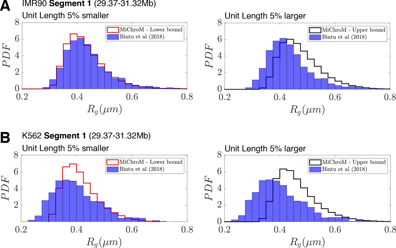
Deviations in the unit of length estimate can account for the differences in the experimental and simulated distributions of radius of gyration .
(A) The distributions of radius of gyration for the experimentally traced IMR90 Segment 1 (A) and K562 Segment 1 (B) (Bintu et al., 2018) are plotted alongside the distribution of radius of gyration from simulation when the unit length of our model (0.165 μm) is 5% smaller or 5% larger.
Figure 3—figure supplement 3

Comparison of the population-averaged contact maps from experimental tracing and simulation for Segment 1.
The 30 kb resolution experimental maps and the 50 kb simulated maps are compared at a resolution of 150 kb. Here, 330 nm is used to define a contact between two loci. (A) The contact map from experimental tracing (Figure 2B) is compared with the simulated contact map (Figure 3B) for closed structures (Cluster 1) with a Pearson’s R of 0.956 and a distance-corrected Pearson’s R (Bianco et al., 2018) of 0.695. (B) The contact map from experimental tracing (Figure 2C) is compared with the simulated contact map (Figure 3C) for open structures (Cluster 2) with a Pearson’s R of 0.916 and a distance-corrected Pearson’s R (Bianco et al., 2018) of 0.531.
Figure 4
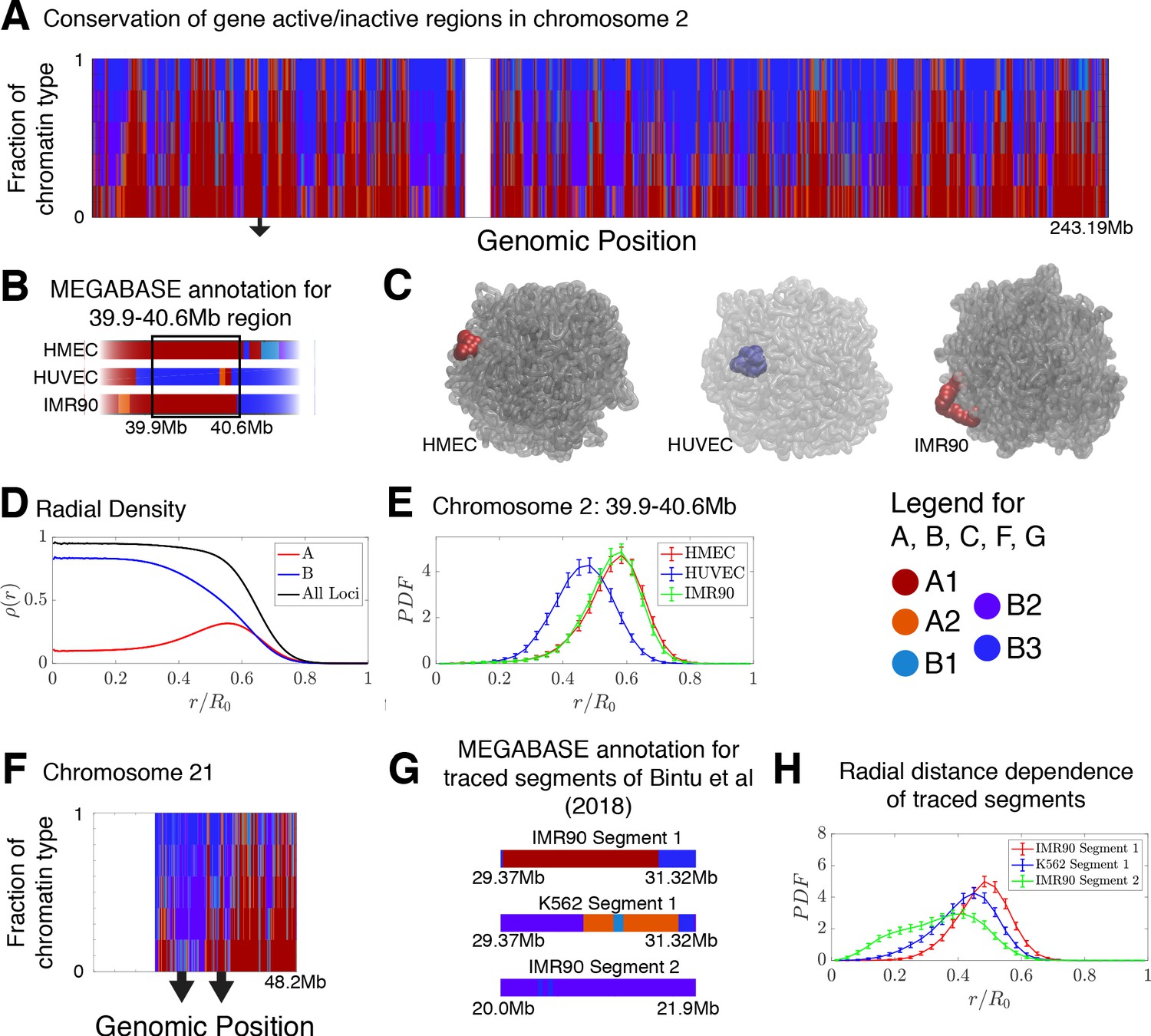
Conservation of compartmentalization across cell types and the radial dependence of marked chromatin.
(A) A stacked bar chart is used to represent the distribution of chromatin type annotations predicted by MEGABASE as a function of the genomic position along chromosome 2 (hg19). The colors correspond the chromatin types given in the Figure Legend. For a given genomic position, the relative height of a particular color indicates the fraction of that particular chromatin type predicted at that locus. (B) The MEGABASE prediction of the chromatin type is shown for the chromatin segment 39.9–40.6 Mb of chromosome 2 for HMEC, HUVEC, and IMR90. A black arrow in (A) highlights the location of this segment. (C) The chromatin segment 39.9–40.6 Mb of chromosome 2 is shown in a representative structure for each of the cell types, where the color of the segment denotes its MEGABASE annotation. For HMEC and IMR90, the segment of chromatin tends toward the chromosome surface, whereas the segment tends toward the interior for HUVEC. (D) The radial density as a function of the normalized radial distance is plotted for A compartment loci, B compartment loci, and all loci for simulations of chromosomes for the HMEC cell type. (E) The probability density functions of the radial distance are shown for the center of mass of the segment 39.9–40.6 Mb of chromosome 2 for HMEC, HUVEC, and IMR90, respectively. (F) A stacked bar chart is used to represent the distribution of chromatin type annotations predicted by MEGABASE as a function of the genomic position along chromosome 21 (hg19). The arrows indicate the locations of the traced segments of Bintu et al., 2018: Segment 1 (29.37–31.32 Mb) and Segment 2 (20.0–21.9 Mb). (G) The MEGABASE annotation of the traced chromatin segments are given for IMR90 and K562. (H) The distribution of radial distances of the center of mass of each traced segment is shown.
Additional files
-
Supplementary file 1
MiChroM parameters for type-to-type interactions.
The energetic parameters are provided in units of ε. We consider five chromatin types (A1, A2, B1, B2, and B3) and a non-specific type (NA).
- https://cdn.elifesciences.org/articles/60312/elife-60312-supp1-v2.docx
-
Transparent reporting form
- https://cdn.elifesciences.org/articles/60312/elife-60312-transrepform-v2.pdf
Download links
A two-part list of links to download the article, or parts of the article, in various formats.
Downloads (link to download the article as PDF)
Open citations (links to open the citations from this article in various online reference manager services)
Cite this article (links to download the citations from this article in formats compatible with various reference manager tools)
Exploring chromosomal structural heterogeneity across multiple cell lines
eLife 9:e60312.
https://doi.org/10.7554/eLife.60312


