Figures and data in The amygdala instructs insular feedback for affective learning

Figures
Tables
Additional files

5 figures, 2 tables and 1 additional file

Figures

Figure 1 with 8 supplements

Download asset Open asset

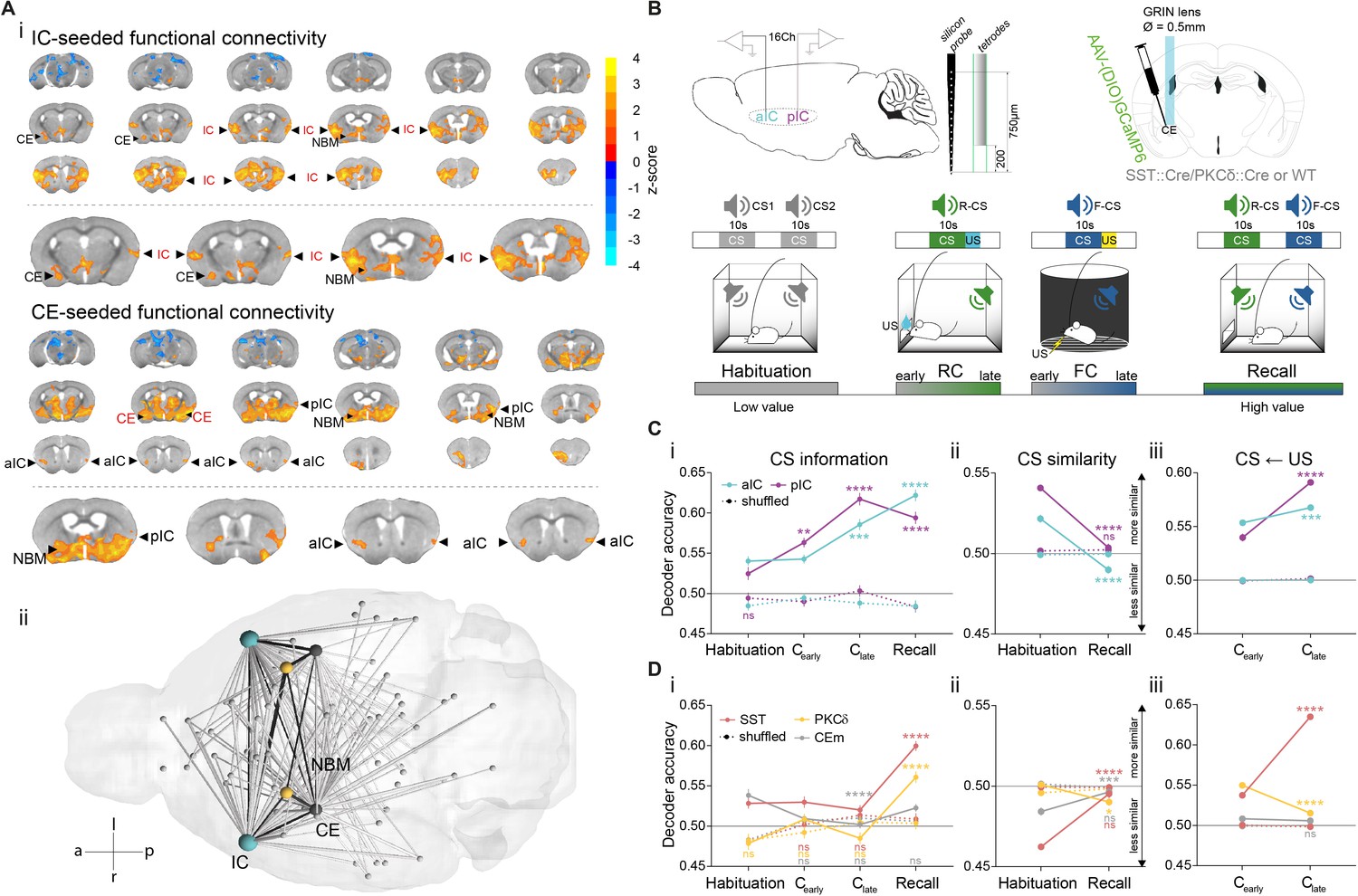
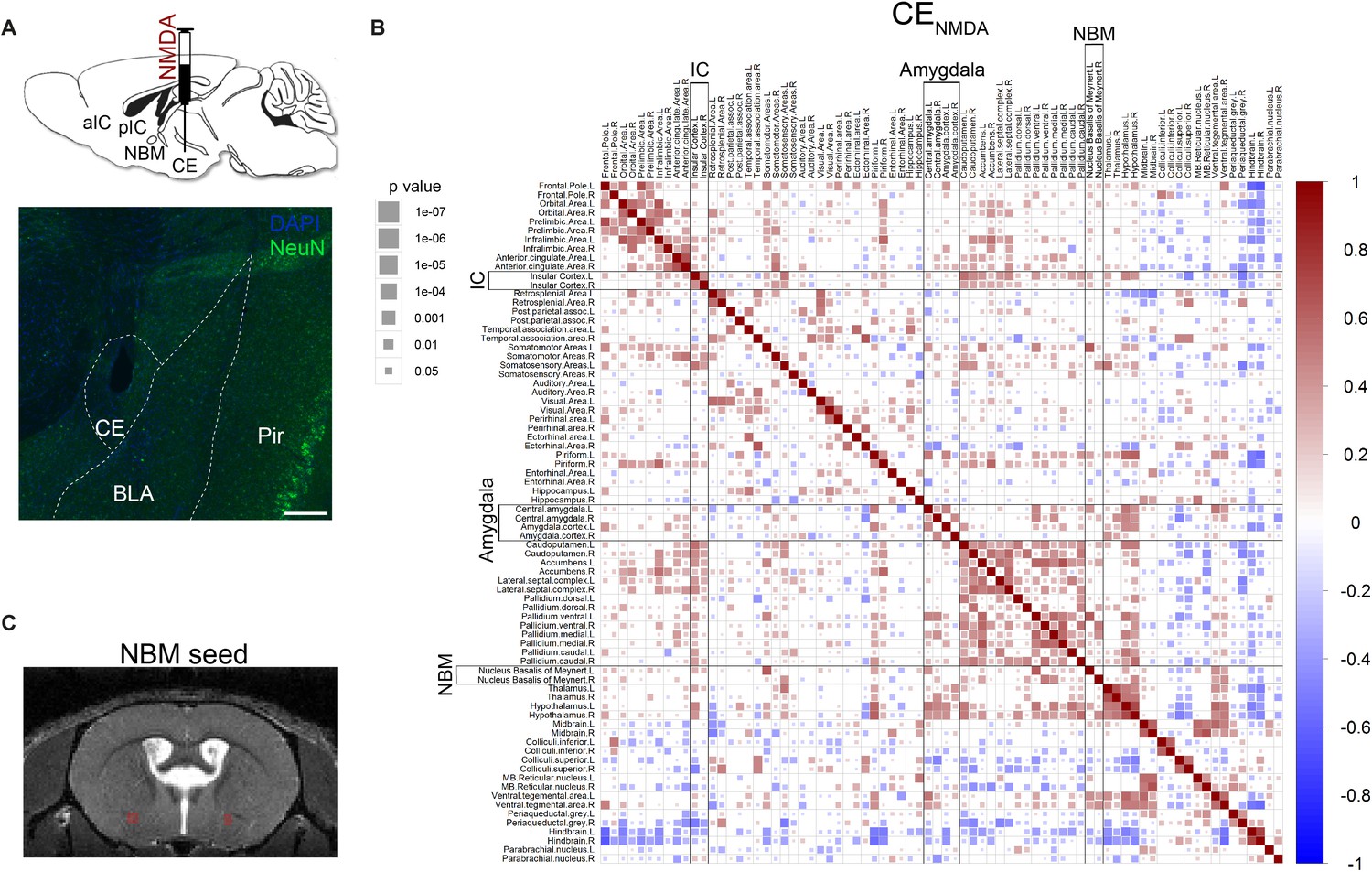
IC and CE are coupled and acquire information on task stimuli.

(A) (i) Seed-based functional connectivity of the bilateral IC (*top*) showed coupling to CE and NBM. Seeding the CE (*bottom*) showed coupling to the aIC, pIC and NBM (radiological view). Significant z-scored correlations to seed nodes are displayed in orange (positive) and blue (negative). (ii) Bottom-view of region-based functional connectivity of ROIs (see correlation matrix in Figure 1—figure supplement 1B). Edge thickness depicts connectivity strength. Only nodes and edges with significant correlations to IC and CE are shown. Edges between IC, CE, and NBM are highlighted in black. (B) Schematic depiction of experimental recordings. *Top, left:* mice were chronically implanted with single-site silicon or multi-site tetrode probes in aIC and pIC. *Top, right:* SST::Cre, PKCδ::Cre, or wild-type mice were chronically implanted with a GRIN lens above CE in animals injected with AAVs carrying GCaMP6. *Bottom:* Experimental timeline of the four-stage discriminatory Pavlovian learning paradigm. (C) (i) Decoder accuracy (Da) of a multi-layer perceptron (MLP) classifier trained to detect CS information in the activity of 200 random draws of 40 neurons per IC subregion for each CS and stage. Mean of both CSs is shown (significant stage x subregion interaction in a two-way ANOVA F_9,6384=13.69, p<0.0001). * Indicates significant differences from the respective habituation stage. (ii) MLP, trained on 400 random draws of neurons as in (i), to detect R(F)-CS, but applied on F(R)-CS within the habituation and recall stages (significant stage x subregion interaction in a two-way ANOVA, F_3,6392=42.10, p<0.0001). * Indicates significant differences from the habituation stage. (iii) Mean Da of an MLP trained on the activity of 400 random draws of 40 neurons per IC subregion to detect R-US or F-US applied on R-CS or F-CS, respectively, within the C_early and C_late stages (significant stage x subregion interaction in a two-way ANOVA F_3,6392=50.14, p<0.0001). * Indicates significant differences from the C_early stage. (D) (i) Da of an MLP trained to detect CS information in the activity of 200 random draws of neurons for each CE population (30 neurons for each CE^SST and CE^PKCδ and seven neurons for CEm), CS and stage. Mean of both CSs is shown (significant stage x population interaction in a two-way ANOVA F_15,9576=9.30, p<0.0001). * Indicates significance as in Ci. (ii) MLP, trained on 400 random draws of neurons as in (i), to detect R(F)-CS, but applied on F(R)-CS within the habituation and recall stages (significant stage x population interaction in a two-way ANOVA, F_5,9588=30.40, p<0.0001). (iii) Mean Da of an MLP trained on the activity of 400 random draws of neurons (30 neurons each for CE^SST and CE^PKCδ, and 10 from CEm) to detect R-US or F-US and applied on R-CS or F-CS, respectively, within the C_early and C_late stages (significant stage x population interaction in a two-way ANOVA F_5,9588=339.60, p<0.0001). Holm-Sidak post hoc for all analyses, ****p<0.0001. Only non-significant differences to shuffled data are explicitly indicated (‘ns’). All data presented as mean ± SEM. Full statistical report in Appendix 1—table 1.

Figure 1—source data 1 Decoding accuracy of an MLP classifier on iterative draws of neurons from IC and CE populations.: https://cdn.elifesciences.org/articles/60336/elife-60336-fig1-data1-v1.xlsx
Download elife-60336-fig1-data1-v1.xlsx

Figure 1—figure supplement 1

Download asset Open asset

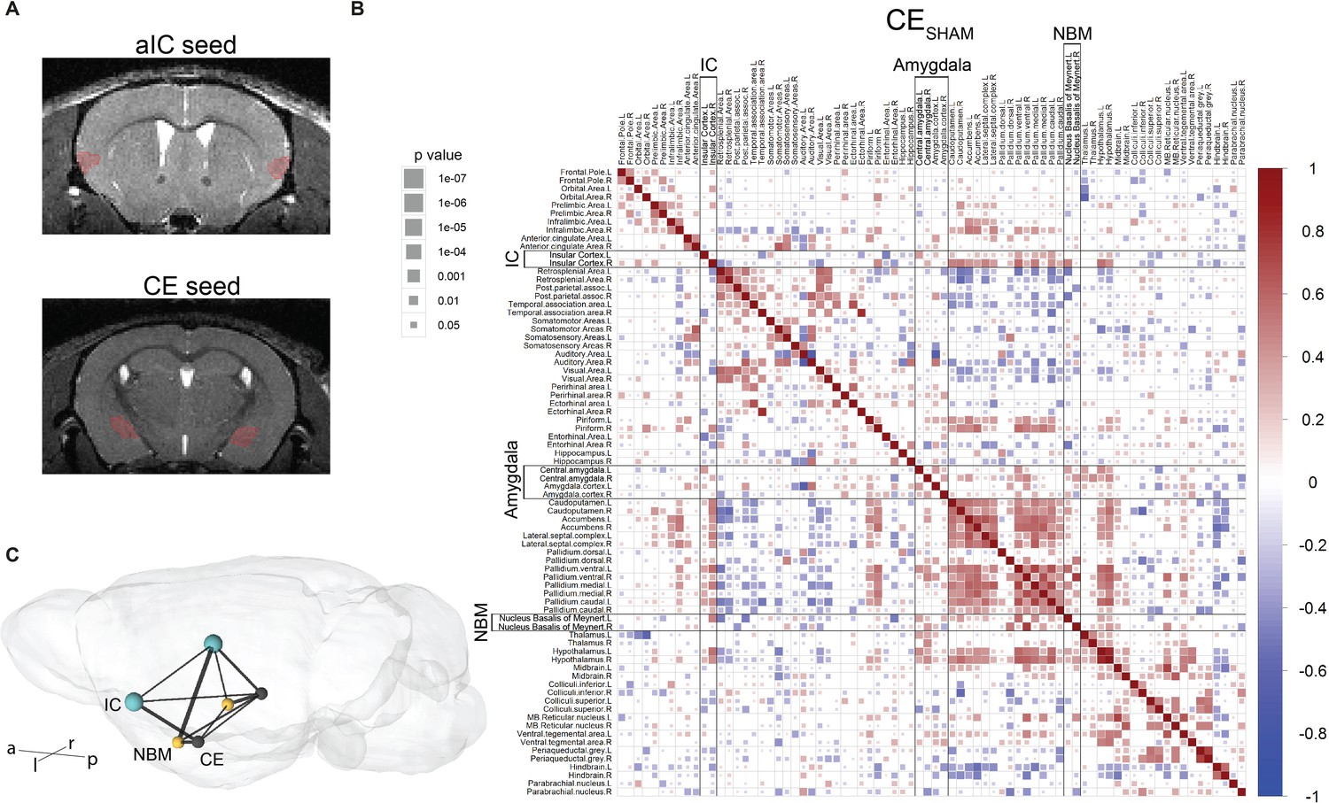
ROI-based functional connectivity of the control group.

(A) Seed region masks used for functional connectivity of the anterior insular cortex (aIC) and central nucleus of amygdala (CE). (B) Functional connectivity in the CE_SHAM group with significant (one sample t-test, p<0.05) Fisher z-transformed Pearson correlation coefficients between each pair of brain regions (blue-to-red scale) is shown (significance of correlations reflected by the size of the square). (C) Region-based functional connectivity of IC, CE, and Nucleus Basalis of Meynert (NBM; from the correlation matrix in B). Edge thickness depicts connectivity strength.

Figure 1—figure supplement 1—source data 1 fMRI cross-correlation matrix of CE_SHAM in Figure 1—figure supplement 1B.: https://cdn.elifesciences.org/articles/60336/elife-60336-fig1-figsupp1-data1-v1.xlsx
Download elife-60336-fig1-figsupp1-data1-v1.xlsx

Figure 1—figure supplement 2

Download asset Open asset

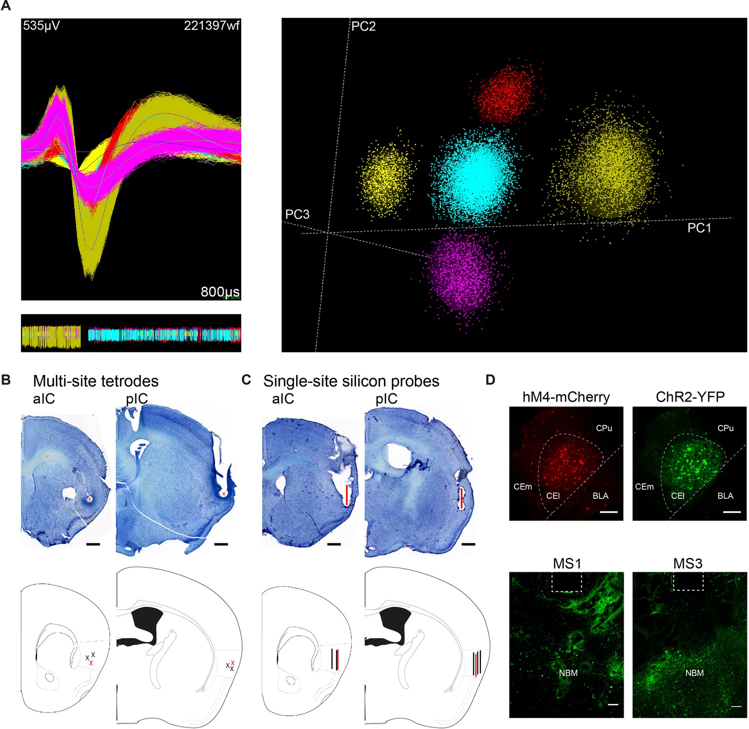
Raw data and histological assessment of IC recordings.

(A) Example waveforms of five single units (*top, left*) and their corresponding representation in PC space (*right*) from two recording sessions on separate days (*bottom, left*). (B) Nissl staining of tissue from an animal implanted with multi-site tetrodes in aIC (*top, left*) and pIC (*top, right*) and corresponding summary schema of all multi-site implantation sites (*bottom*). Red ‘X’s indicate corresponding electrolytic lesion sites in both staining and schema. Scalebar = 500 μm. (C) Nissl staining from tissue of animals implanted with single-site 16 Channel silicon probes in aIC (*top, left*) and pIC (*top, right*) and corresponding summary schema of all single-site implantation sites (*bottom*). Red lines indicate corresponding electrolytic lesion sites between staining and schema. Scalebar = 500 μm. (D) Viral expression of Cre-dependent hM4-mCherry (*top, left*) and ChR2-YFP (*top, right*) in the CE and corresponding projection fields with optic fiber (400 μm) position above NBM (*bottom*) in two multi-site recorded PKCδ::Cre animals. Scalebar = 100 μm.

Figure 1—figure supplement 3

Download asset Open asset

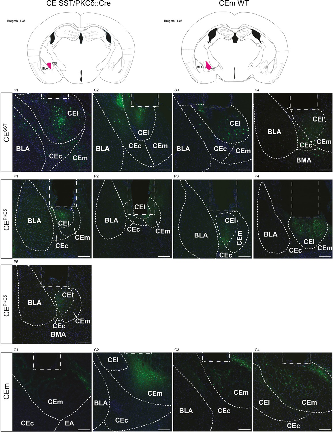
Histology of calcium imaging cohorts.

Schematic coronal sections of targeted areas and from all calcium recording groups. SST::Cre and PKCδ::Cre mice were injected with AAV-hSyn-DIO-GCaMP6f in the right lateral central amygdala (CEl). WT mice were injected with AAV-hSyn-GCaMP6m in the right medial central amygdala (CEm). Rectangular dashed shape indicates GRIN lens placement (Ø=500 µm); scalebar = 200 µm. BLA – basolateral amygdala, BMA – basomedial amygdala, CEc, capsular part of central amygdala.

Figure 1—figure supplement 4

Download asset Open asset

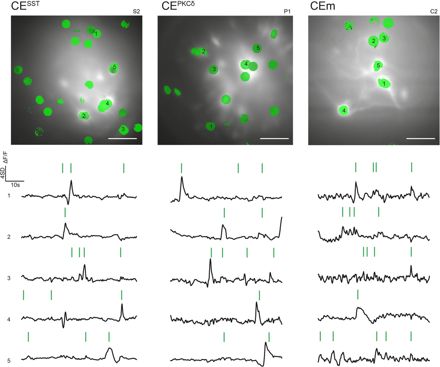
Representative FOVs and activity from CE calcium imaging.

Green overlay corresponds to automatically detected and manually selected units to exclude artifacts. Scalebar = 100 µm (*top*). Five representative traces from each FOV with detected calcium events in green. Vertical scalebar corresponds to four standard deviations of ΔF/F calcium signal, horizontal scalebar corresponds to 10 s (*bottom*).

Figure 1—figure supplement 5

Download asset Open asset

Responses to Pavlovian learning task stimuli in IC.

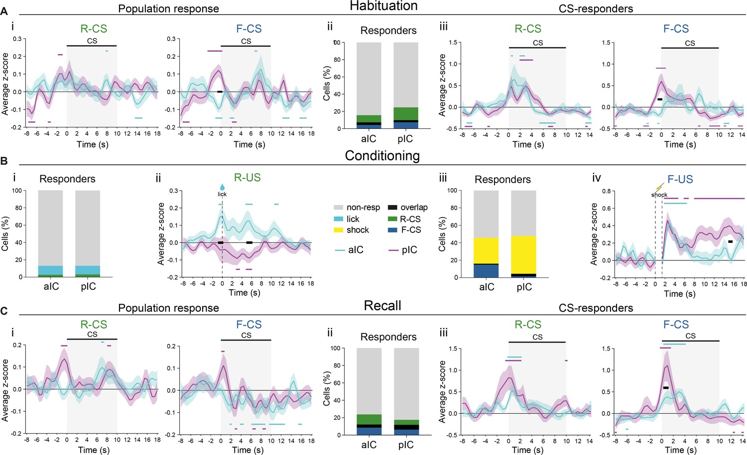
In all panels, black lines indicate significant differences (p<0.05) between subregions, as determined by Holm-Sidak post hoc analyses, while colored lines indicate significant differences (p<0.05) from zero for each subregion, as determined by one-sample t-tests. All data presented as mean ± SEM. (A) (i) PETH of CS-evoked population responses of IC subregions for (*left*) R-CS (significant effect of time in a two-way RM ANOVA, F_52,11180=1.61, p=0.0037) and (*right*) F-CS (significant time x subregion interaction in a two-way RM ANOVA, F_52,11076=2.23, p<0.0001) at habituation. (ii) Percentage of neurons responsive to task stimuli, determined by trial-averaged neuronal responses above a z-score of 1.65 at habituation. (iii) PETH of CS-evoked responses of IC responders (from ii) for (*left*) R-CS (significant effect of time in a two-way RM ANOVA, F_52,1664=5.682, p<0.0001) and (*right*) F-CS (significant time x subregion interaction in a two-way RM ANOVA, F_52,884=1.782, p=0.0007) at habituation. (B) (i) Percentage of neurons responsive to task stimuli, as determined by trial-averaged neuronal responses above a z-score of 1.65 in RC. (ii) Average z-scored population responses of IC subregions as PETH upon R-US (significant time x subregion interaction in a two-way RM ANOVA, F_52,14248=1.87, p=0.0002). (iii) Percentage of neurons responsive to task stimuli, as determined by trial-averaged neuronal responses above a z-score of 1.65 in FC. (iv) Average z-scored population responses as PETH of IC subregions upon F-US (significant time x subregion interaction in a two-way RM ANOVA, F_50,7100=2.29, p<0.0001). (C) (i) PETH of CS-evoked population responses at recall of IC subregions for (*left*) R-CS (no significant effect in a two-way RM ANOVA) and (*right*) F-CS (significant effect of time in a two-way RM ANOVA, F_52,14560=2.42, p<0.0001). (ii) Percentage of neurons responsive to task stimuli, determined by trial-averaged neuronal responses above a z-score of 1.65 at recall. (iii) PETH of CS-evoked responses of IC responders (from ii) for (*left*) R-CS (significant effect of time in a two-way RM ANOVA, F_52,1924=2.984, p<0.0001) and (*right*) F-CS (significant time x subregion interaction in a two-way RM ANOVA, F_52,1716=2.159, p<0.0001) at recall. Full statistical report in Appendix 1—table 1.

Figure 1—figure supplement 6

Download asset Open asset

Responses to Pavlovian learning task stimuli in CE.

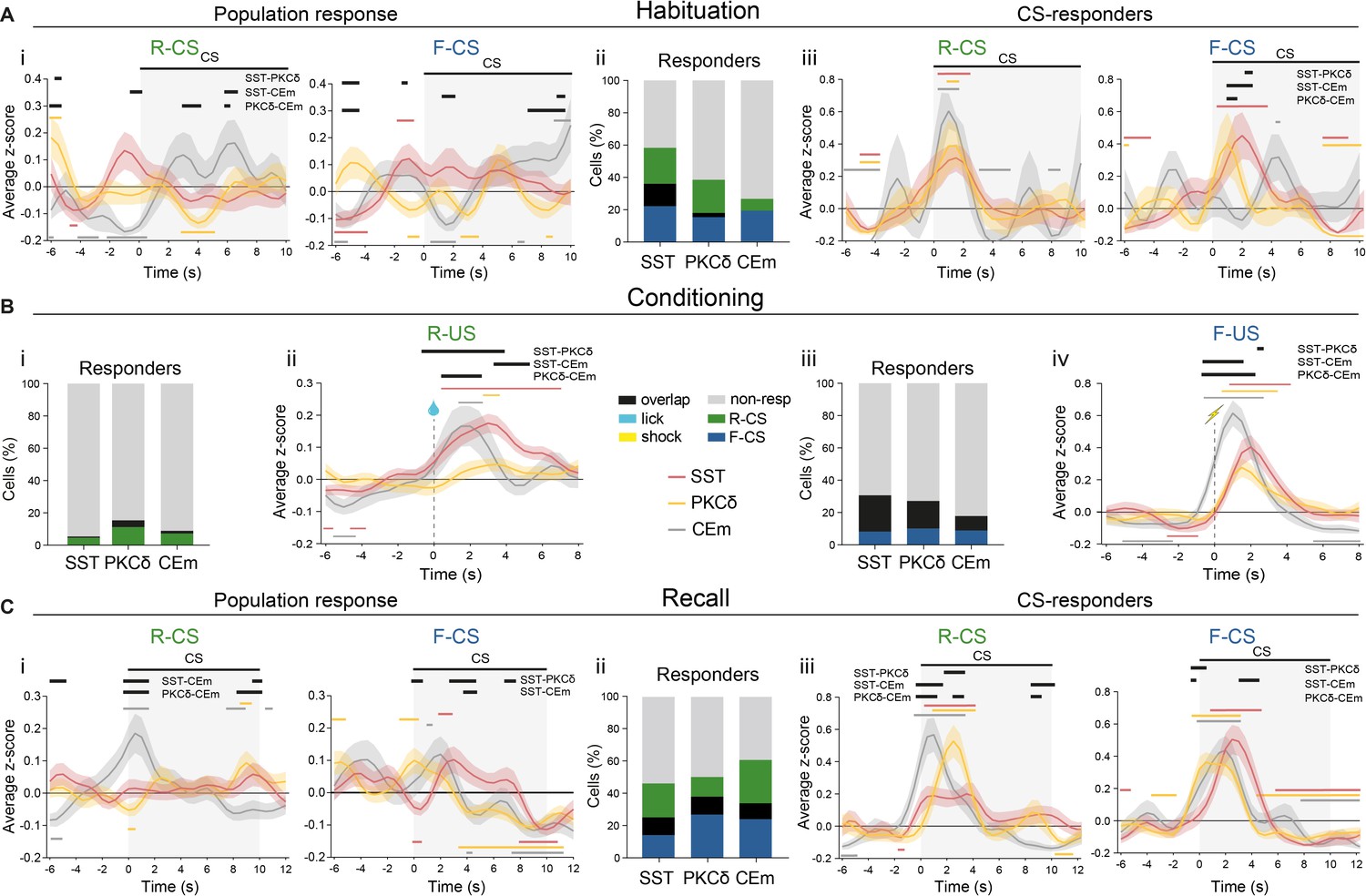
In all panels, black lines indicate significant differences (p<0.05) between populations, as determined by Holm-Sidak post hoc analyses, while colored lines indicate significant differences (p<0.05) from zero for each population, as determined by one-sample t-tests. All data presented as mean ± SEM. (A) (i) PETH of CS-evoked population responses of CE subpopulations for (*left*) R-CS (significant time x population interaction in a two-way RM ANOVA, F_64,3232=2.76, p<0.0001) and (*right*) F-CS (significant time x population interaction in a two-way RM ANOVA, F_64,4032=2.43, p<0.0001) at habituation. (ii) Percentage of neurons responsive to task stimuli, as determined by trial-averaged neuronal responses above a z-score of 1.65 at habituation. (iii) PETH of CS-evoked population responses of CE responders (from ii) for (*left*) R-CS (significant effect of time in a two-way RM ANOVA, F_32,800=7.436, p<0.0001) and (*right*) F-CS (significant time x population interaction in a two-way RM ANOVA, F_64,1056=1.721, p=0.0005) at habituation. (B) (i) Percentage of neurons responsive to task stimuli, as determined by trial-averaged neuronal responses above a z-score of 1.65 in RC. (ii) Average z-scored population responses of CE subpopulations as PETH upon R-US (significant time x population interaction in a two-way RM ANOVA, F_56,3976=2.45, p<0.0001). (iii) Percentage of neurons responsive to task stimuli, as determined by trial-averaged neuronal responses above a z-score of 1.65 in FC. (iv) Average z-scored population responses as PETH of CE subpopulations upon F-US (significant time x population interaction in a two-way RM ANOVA, F_56,4480=4.22, p<0.0001). (C) PETH of CS-evoked population responses at recall of CE subpopulations for (*left*) R-CS (significant time x population interaction in a two-way RM ANOVA, F_72,9684=2.81, p<0.0001) and (*right*) F-CS (significant time x population interaction in a two-way RM ANOVA, F_72,9072=2.01, p<0.0001). (ii) Percentage of neurons responsive to task stimuli, as determined by trial-averaged neuronal responses above a z-score of 1.65 at recall. (iii) PETH of CS-evoked responses at recall of CE responders (from ii) for (*left*) R-CS (significant time x population interaction in a two-way RM ANOVA, F_72,2952=3.577, p<0.0001) and (*right*) F-CS (significant time x population interaction in a two-way RM ANOVA, F_72,3240=2.273, p<0.0001) at recall. All data presented as mean ± SEM. Full statistical report in Appendix 1—table 1.

Figure 1—figure supplement 7

Download asset Open asset

Valence-specific mapping of CS and US features in IC–CE circuitry.

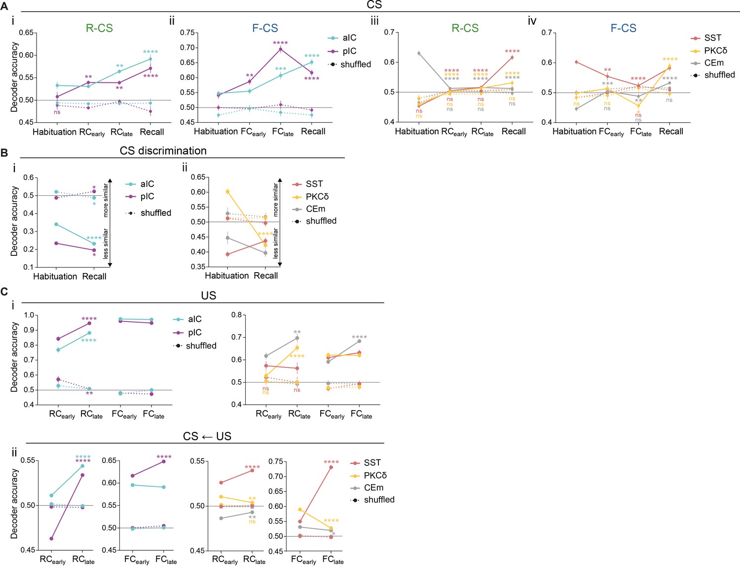
(A) Decoder accuracy (Da) of an MLP trained to detect CS information in the activity of 200 random draws of 40 neurons per IC subregion for (i) R-CS (significant stage x subregion interaction in a two-way ANOVA, F_9,3184=5.68, p<0.0001) and (ii) F-CS (significant stage x subregion interaction in a two-way ANOVA, F_9,3184=11.50, p<0.0001) and 200 random draws of CE neurons (30 for each CE^SST and CE^PKCδ and seven for CEm) per stage upon (iii) R-CS (significant stage x population interaction in a two-way ANOVA, F_15,4776=29.17, p<0.0001) and (iv) F-CS (significant stage x population interaction in a two-way ANOVA, F_15,4776=7.93, p<0.0001). * Indicate significant differences from the respective habituation stage within each subregion/population by a designated post hoc test. Only non-significant differences to shuffled data are explicitly indicated (‘ns’). (B) Alternative classification approach to Figure 1Cii, Dii for CS discrimination. An MLP was trained to discriminate between preCS, R-CS, and F-CS. Graphs show average Da for classifying the correct CS, given the bin is within any CS period and was classified as such. (i) 200 random draws of 40 neurons each for aIC and pIC (significant stage x subregion interaction in a two-way ANOVA, F_3,1592=18.53, p<0.0001) and (ii) of 30 neurons from CE^PKCδ and CE^SST and 7 CEm neurons (significant stage x population interaction in a two-way ANOVA, F_5,2366=15.58, p<0.0001). (C) (i) Da of an MLP trained to detect US information in the activity of 200 random draws of 40 neurons per IC subregion, 30 for CE^PKCδ and CE^SST and 10 neurons for CEm for R-US (IC: significant stage x subregion interaction in a two-way ANOVA, F_3,1592=16.06, p<0.0001; CE: significant stage x population interaction in a two-way ANOVA, F_5,2228=5.40, p<0.0001) and F-US (IC: significant effect of subregion in a two-way ANOVA, F_3,1592=1619.00, p<0.0001, CE: significant stage x population interaction in a two-way ANOVA, F_5,2388=4.01, p=0.0013). This classifier was used for the CS←US task. (ii) Projection of US properties by application of the MLP from (i) to the respective CS (IC/RC: significant stage x subregion interaction in a two-way ANOVA, F_9,3192=242.50, p<0.0001; IC/FC: significant stage x subregion interaction in a two-way ANOVA, F_9,3192=9.97, p<0.0001; CE/RC: significant stage x population interaction in a two-way ANOVA, F_5,4788=18.39, p<0.0001; CE/FC: significant stage x population interaction in a two-way ANOVA, F_5,4788=603.30, p<0.0001). All data presented as mean ± SEM. Full statistical report in Appendix 1—table 1.

Figure 1—figure supplement 8

Download asset Open asset

Performance-dependent responses to Pavlovian learning task stimuli in IC and CE.

In all panels, black lines indicate significant differences (p<0.05) between subregions/populations, as determined by Holm-Sidak post hoc analyses, while colored lines indicate significant differences (p<0.05) from zero for each subregion/population, as determined by one-sample t-tests. All data presented as mean ± SEM. (A) Performance of individual mice in the reward (*left*) and fear (*right*) domain in IC and CE, as determined by the p-value from t-tests comparing the number of port visits (reward) and freezing episode onsets (fear) before and during CS presentations at recall. Color assignment of individual points according to a median split of p-values (red – performer, gray – non-performer). The median performer was assigned to the ‘performer’ group if its p-value was ≤0.5. (B) PETH of population responses according to performance for aIC upon (i) R-US (significant time x performance interaction in a two-way RM ANOVA, F_52,7592=1.63, p=0.0029) and (ii) F-US (significant time x performance interaction in a two-way RM ANOVA, F_50,3950=2.47, p<0.0001), and of pIC upon (iii) R-US (significant time x performance interaction in a two-way RM ANOVA, F_52,6552=9.86, p<0.0001) and (iv) F-US (significant time x performance interaction in a two-way RM ANOVA, F_50,3050=3.27, p<0.0001). (C) PETH of population responses according to performance for aIC upon (i) R-CS (significant time x performance interaction in a two-way RM ANOVA, F_52,8268=2.09, p<0.0001) and (ii) F-CS (significant time x performance interaction in a two-way RM ANOVA, F_52,8268=1.36, p=0.0434) and for pIC upon (iii) R-CS (no significant effect in a two-way RM ANOVA) and (iv) F-CS (significant time x performance interaction in a two-way RM ANOVA, F_52,6188=1.81, p=0.0003). (D) (i-iii) PETH of population responses according to performance at recall for CE^SST upon R-US (*top*, significant time x performance interaction in a two-way RM ANOVA, F_28,3052 = 2.33, p<0.0001; *middle,* significant effect of performance in a two-way RM ANOVA, F_1,109=5.70, p=0.0187) and (*bottom*) F-US (significant time x performance interaction in a two-way RM ANOVA, F_28,1344=2.22, p=0.0003). (iv-vi) PETH of population responses according to performance at recall for CE^PKCδ upon R-US (*top*, significant time x performance interaction in a two-way RM ANOVA, F_28,3192=3.07, p<0.0001; *middle,* significant time x performance interaction in a two-way RM ANOVA, F_28,3220=1.56, p=0.0262) and (*bottom*) F-US (significant time x performance interaction in a two-way RM ANOVA, F_28,1848=2.96, p<0.0001). (vii-ix) PETH of population responses according to performance at recall for CEm upon R-US (*top*, significant effect of time in a two-way RM ANOVA, F_28,1512=3.95, p<0.0001; *middle,* significant time x performance interaction in a two-way RM ANOVA, F_28,1512=2.92, p<0.0001) and (*bottom*) F-US (significant effect of time in a two-way RM ANOVA, F_28,1204=22.73, p<0.0001). Full statistical report in Appendix 1—table 1.

Figure 2 with 7 supplements

Download asset Open asset

IC-CE information flow facilitates conditioned responding.

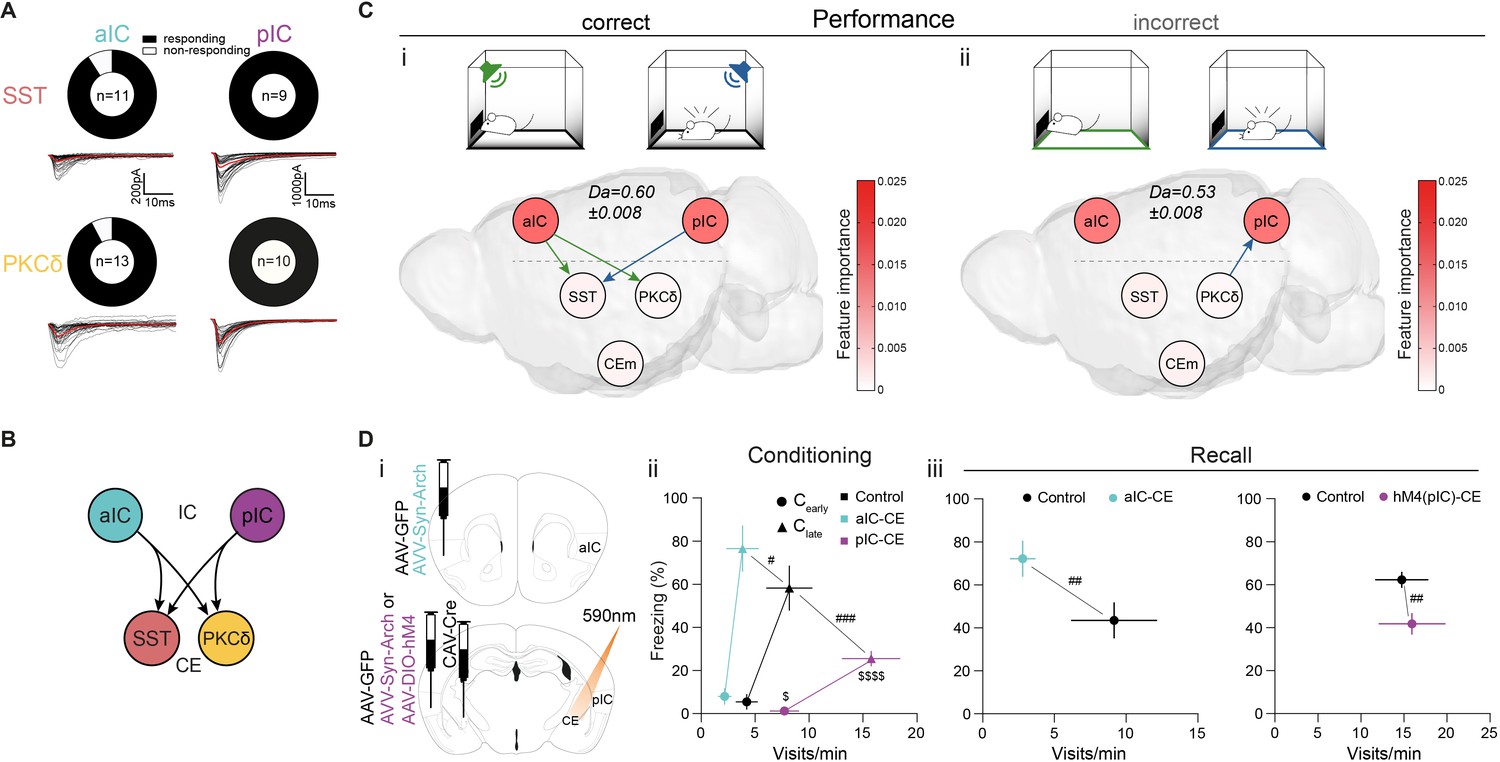
(A) Fraction of SST⁺ and PKCδ⁺ neurons in CEl that responded with EPSCs upon optogenetic stimulation of aIC or pIC input. (B) Scheme for IC inputs to CEl populations. (C) Performance-dependent transfer entropy (TE) between IC and CE nodes for (i) correct (port visits during R-CS and freezing episodes during F-CS) and (ii) incorrect (port visits or freezing outside of corresponding CS) behavioral episodes (±2 s of bin containing behavioral episode onset). RF Decoder accuracy (Da) for decoding behavioral episodes shown above networks. Node color corresponds to RF-associated feature importance, indicating information most relevant for RF classification (see Figure 2—figure supplement 2Ai). (D) (i) Experimental approach to functionally dissect aIC and pIC inputs to CE during a Pavlovian learning task. (ii) Behavioral performance of optogenetic experimental groups in C_early and C_late stages. Significant MANOVA in C_early (F_2,44=3.60, p=0.0126) and C_late (F_2,44=6.43, p=0.0004). (iii) Behavioral performance of the optogenetic (left) and chemogenetic (hM4(pIC)–CE, right) IC–CE treatment cohorts during manipulation-free recall. Significant MANOVA at recall for the aIC-CE manipulation (F_1,13=8.18, p=0.005) and pIC-CE manipulation (F_1,17=6.81, p=0.0067). Data shown as mean ± SEM. n_GFP=9/12 n_aIC–CE=7, n_pIC–CE=9/8. Holm post hoc as difference to control is noted as #, between manipulation groups is noted as $. #/$p<0.05, ##p<0.01, ###p<0.001, $$$$p<0.0001. Full statistical report in Appendix 1—table 1.

Figure 2—source data 1 Approach and avoidance behavior during conditioning and recall in chemogenetic pIC–CE and aIC-pIC manipulation cohorts.: https://cdn.elifesciences.org/articles/60336/elife-60336-fig2-data1-v1.xlsx
Download elife-60336-fig2-data1-v1.xlsx

Figure 2—figure supplement 1

Download asset Open asset

Anatomical and functional assessment of IC–CE connectivity.

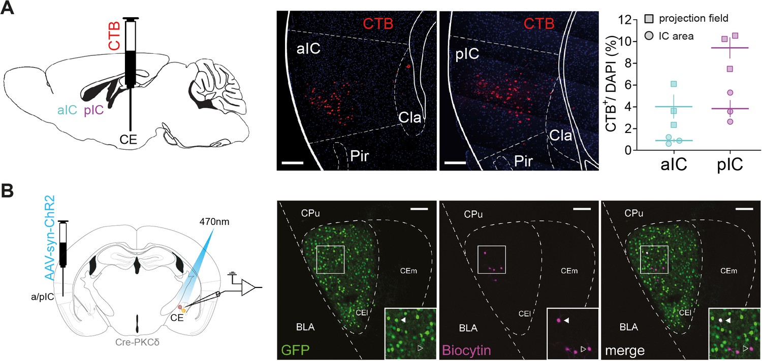
(A) Stereotactic injection of fluorescently labelled CTB into CE (*left*) with representative backlabeling in aIC and pIC (*middle*) and quantification (*right*). Each data point represents a single animal. (B) To assess synaptic connectivity between IC subregions and CE subpopulations in Figure 2A, PKCδ::Cre mice received injections of AAVs carrying Cre-dependent GFP into CE and syn-ChR2 into aIC or pIC (*left*). Exemplary slice showing GFP expression in CE^PKCδ (green) and biocytin-filled fluorescently labelled streptavidin-stained patched neurons (magenta) (*right*).

Figure 2—figure supplement 2

Download asset Open asset

Pavlovian learning task stimulus distributions in the IC–CE network are reshaped by performance and CE^PKCδ.

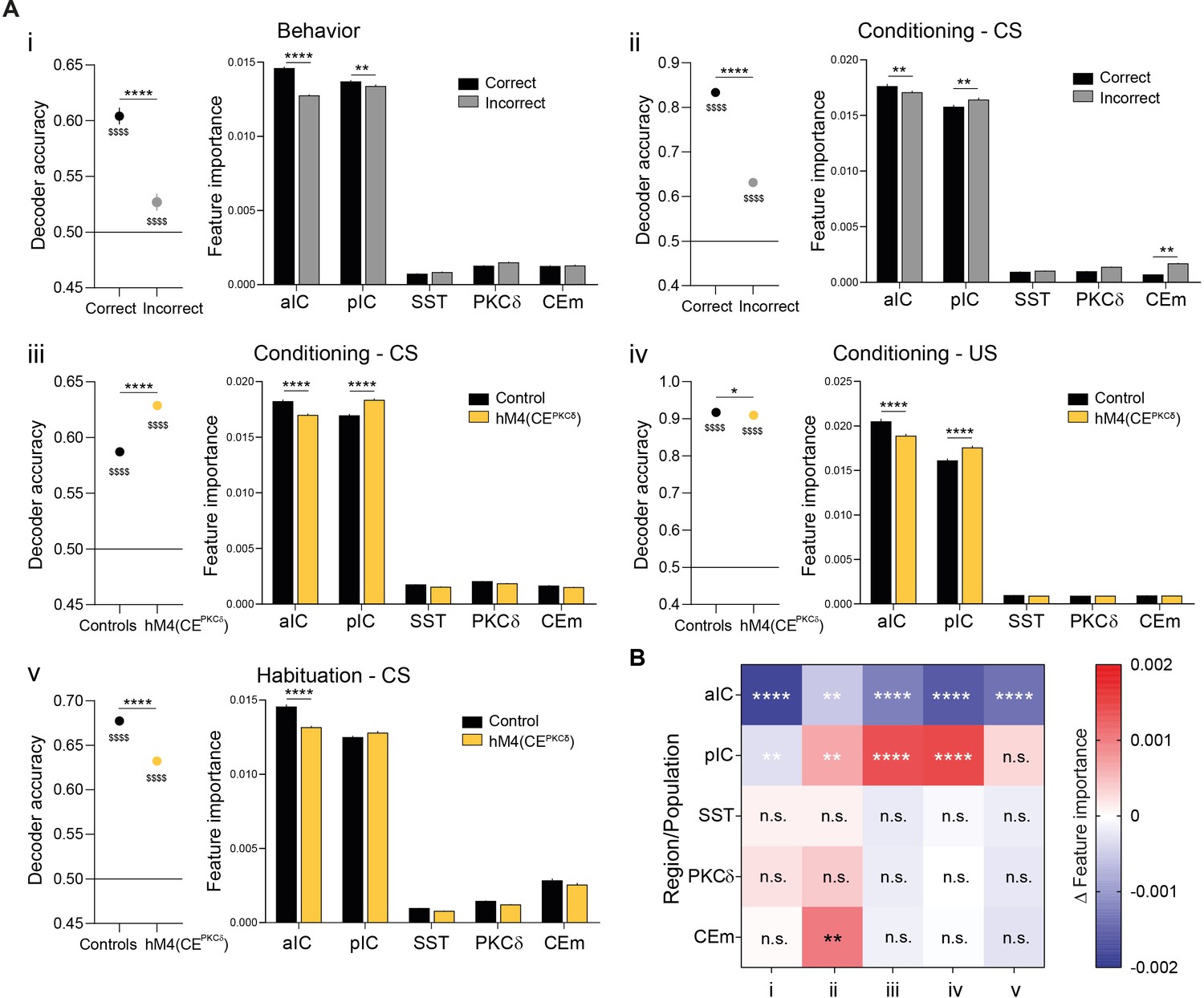
(A) RF Da (*left*) and associated feature importance distribution (*right*) for (i) correct/incorrect behavior during conditioning and recall (one-way ANOVA, F_9,156190=5184.00, p<0.0001), (ii) correct/incorrect CS in conditioning (one-way ANOVA, F_9,73454=2437.00, p<0.0001), (iii) CS in conditioning (one-way ANOVA, F_9,77790=5185.00, p<0.0001), (iv) US in conditioning (one-way ANOVA, F_9,77821=2126.00, p<0.0001) and (v) CS in habituation for control and hM4(CE^PKCδ) conditions (one-way ANOVA, F_9,77619=1766.00, p<0.0001). For Da, * indicates a significant difference as determined by two-sample t-tests, $ indicates a significant difference as determined by one-sample t-tests to random (0.5). For feature importance, Holm-Sidak post hoc was used for all analyses. *p<0.05, **p<0.01, ****/$$$$p<0.0001. (B) Summary of differential feature importance between conditions. Colors were used for all TE network projections.

Figure 2—figure supplement 3

Download asset Open asset

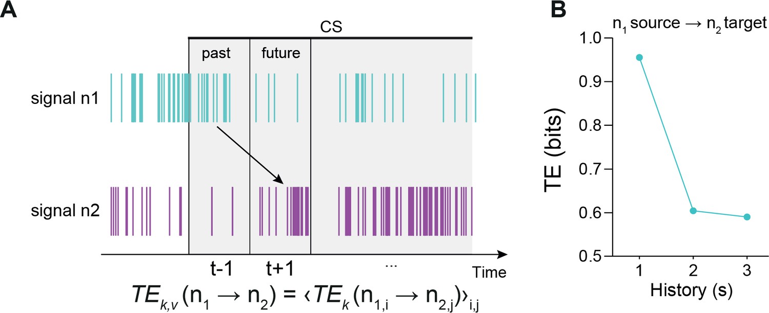
Illustration for quantifying TE and assessment of TE parameter space.

(A) Principle of the quantification of TE between neuron n₁ and neuron n_2, where k refers to past states and i and j label the sample subset of n_1,i and n_2,j of size v in each region. n₂ future signal (time = t+1) can be predicted from the pattern of past activity (time = t-1) in n₁. (B) Mean TE between all pairs of neurons for each CS-type and stage (RC, FC, recall), calculated for the entire network for 1 s binned data with history windows of 1, 2, or 3 s.

Figure 2—figure supplement 4

Download asset Open asset

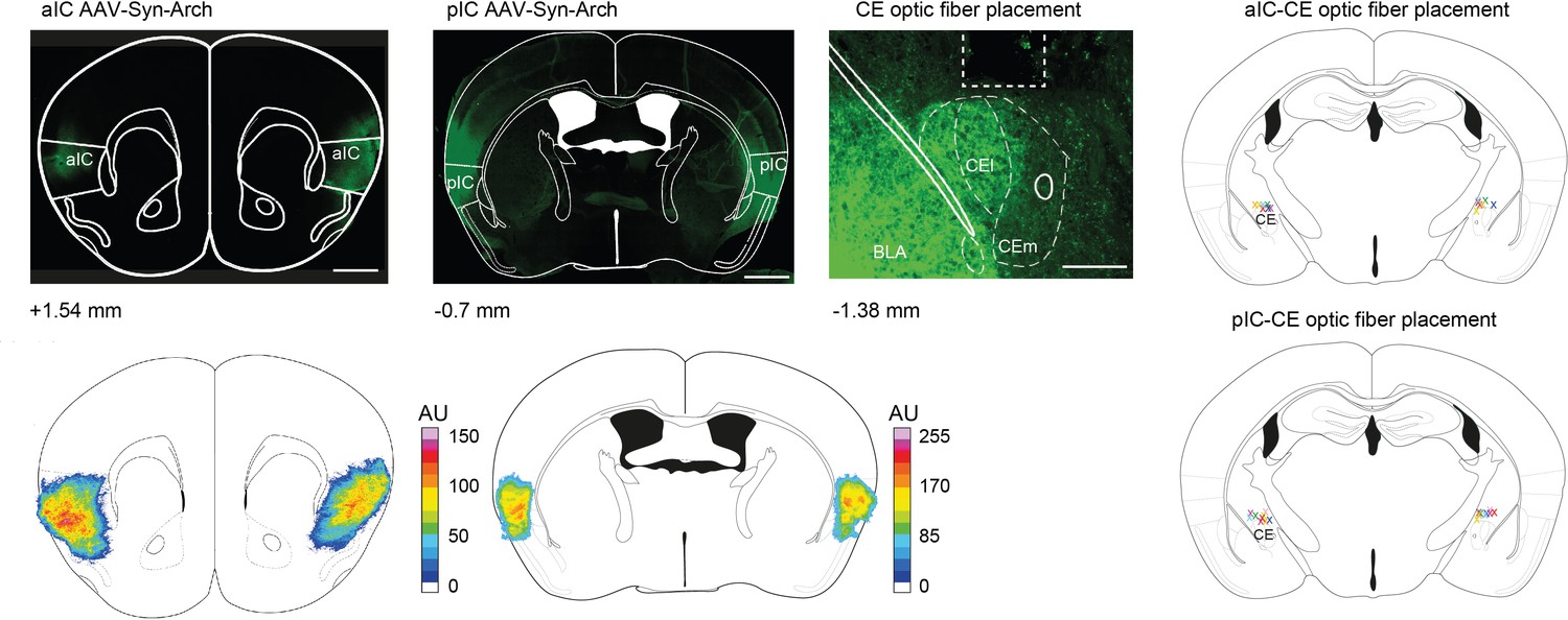
Histological assessment of optogenetic IC–CE manipulation cohorts.

(*top, left*) Exemplary pictures of AAV-Syn-Arch injection sites in aIC and pIC (scalebar = 900 µm) and optic fiber placement above CE (scalebar = 100 µm). (*bottom, left*) Representation of the injection spread in aIC and pIC; heatmap corresponds to the fluorescence intensity. (*right*) Schematic placement of the optic fiber tip above CE marked with ‘x’.

Figure 2—figure supplement 5

Download asset Open asset

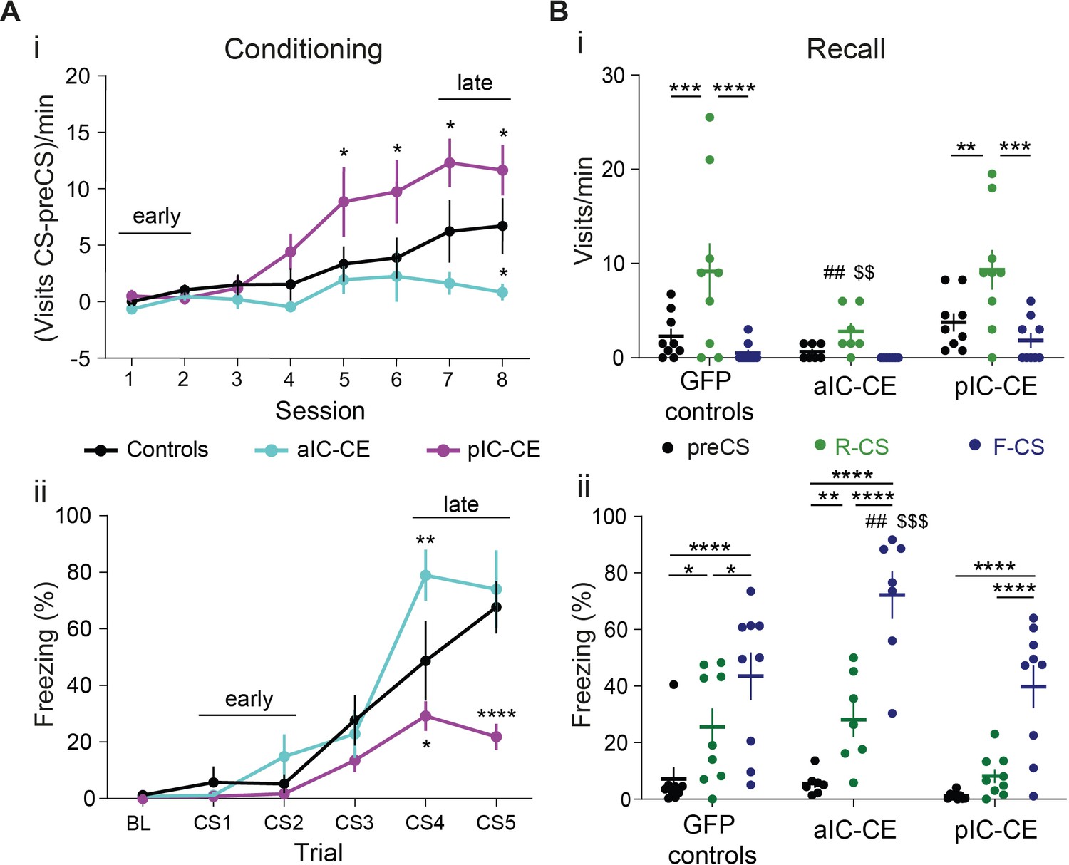
Valence-specific conditioned responses of optogenetic IC–CE manipulation cohorts.

(A) (i) Approach behavior in the RC stage quantified by the differential rate of port visits per minute (port visits/min during CS – port visits/min before CS onset)(significant session x treatment interaction in a two-way RM ANOVA, F_14,154=3.40, p<0.0001). (ii) Avoidance behavior in the FC stage quantified as the percent of time spent freezing during baseline (1 min) and each CS presentation (10 s) (significant treatment x trial interaction in a two-way RM ANOVA, F_10,110=4.71, p<0.0001). (B) Quantification of CS-specific (i) approach (visits/min) (significant effect of treatment in a two-way RM ANOVA, F_2,22=3.95, p=0.0343) and (ii) avoidance behavior (percent of time spent freezing) (significant CS x treatment interaction in a two-way RM ANOVA, F_4,44=3.17, p=0.0225) during a single recall session with four presentations per R-CS and F-CS, without optogenetic manipulation of aIC/pIC–CE pathways. Holm-Sidak post hoc was used for all analyses. */#/$p<0.05, **/##/$$p<0.01, ***/$$$p<0.001, ****p<0.0001, where ‘#’ indicates comparison to the control and ‘$’ comparison to the other treatment group; n_GFP=9 n_aIC–CE=7, n_pIC–CE=9. All data presented as mean ± SEM. Full statistical report in Appendix 1—table 1.

Figure 2—figure supplement 6

Download asset Open asset

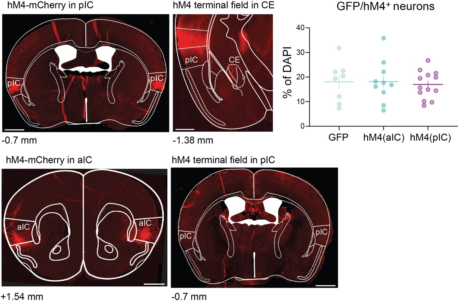
Histological verification of the chemogenetic pIC–CE and aIC–pIC manipulation cohorts.

(*left*) Exemplary pIC and aIC AAV-DIO-hM4-mCherry injection site and (*middle*) terminal hM4-mCherry field in CE and pIC; scalebar = 900 (full sections) and 100 µm (zoom-in). (*right*) Quantification of GFP and hM4 infection rate in aIC and pIC presented as percent of GFP/hM4 positive neurons over DAPI (data shown as mean ± SEM).

Figure 2—figure supplement 7

Download asset Open asset

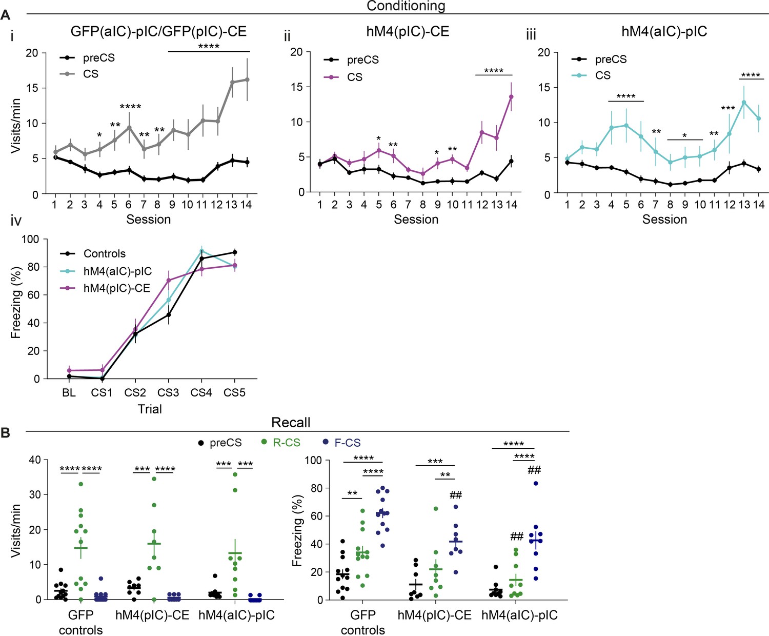
Valence-specific conditioned responses of chemogenetic pIC–CE and aIC–pIC manipulation cohorts.

(A) Learning curves of the aIC–pIC and pIC–CE cohorts for approach behavior of the (i) control (significant CS x session interaction in a two-way RM ANOVA, F_13,130=5.97, p<0.0001), (ii) hM4(pIC)-CE (significant CS x session interaction in a two-way RM ANOVA, F_13,91=9.07, p<0.0001) and (iii) hM4(aIC)-pIC groups (significant CS x session interaction in a two-way RM ANOVA, F_13,104=3.30, p=0.0003). (iv) Learning curves of avoidance behavior of control and treatment groups during the FC stage (significant effect of trial in a two-way RM ANOVA, F_5,125=174.70, p<0.0001). (B) (i) Quantification of CS-specific (*left*) approach (significant effect of CS in a two-way RM ANOVA, F_2,36=31.88, p<0.0001) and (*right*) avoidance behavior (significant effect of treatment in a two-way RM ANOVA, F_1,18=8.65, p=0.0087) at drug-free recall in mice that underwent chemogenetic pIC–CE inhibition during conditioning. n_GFP = 12 n_{hM4(pIC–CE)}=8. (ii) Quantification of CS-specific (*left*) approach (significant effect of CS in a two-way RM ANOVA, F_2,38=30.32, p<0.0001) and (*right*) avoidance behavior (significant effect of treatment in a two-way RM ANOVA, F_1,19=15.80, p=0.0008) at drug-free recall in mice that underwent chemogenetic aIC–pIC inhibition during conditioning. n_Controls = 12, n_hM4(aIC)-pIC=9. Note that the control group was shared between the hM4(pIC)-CE and hM4(aIC)-pIC cohorts, as they were trained in parallel. Holm-Sidak post hoc was used for all analyses. */#/$p<0.05, **/##p<0.01, ***p<0.001, ****p<0.0001, where ‘#’ indicates comparison to the control group. All data presented as mean ± SEM. Full statistical report in Appendix 1—table 1.

Figure 3 with 2 supplements

Download asset Open asset

Learning establishes a performance-linked intra-cortical hierarchy.

(A) TE networks generated from CSs during which correct (i) and incorrect/no (ii) behavior occurred during CS presentations. RF decoder accuracy (Da) for decoding correct/incorrect CSs shown above network. Node color corresponds to feature importance from RF classification. (B) (i) Scheme of recordings from aIC and pIC multi-site implanted animals, examined for interregional interactions at the habituation and recall stages. (ii, iii) STA from the (ii) habituation and (iii) recall stages of 200 ms pIC LFP traces centered around the occurrence of 2388 preCS/2526 CS (habituation) and 7132 preCS/6920 CS (recall) aIC spikes. (iv, v) pIC LFP power-normalized SFC of STAs for (iv) habituation and (v) recall. (C) (i) Experimental strategy for the chemogenetic inhibition of the aIC–pIC pathway. (ii) Quantification of behavioral performance in reward and fear domains at recall with a significant MANOVA (F_1,18=3.64, p=0.0471), n_Controls=12, n_M4(aIC)-pIC=9. Data shown as mean ± SEM. Holm post hoc as difference to control, #p<0.05. Full statistical report in Appendix 1—table 1. (D) (i) TE network of incorrect CS (from Aii), with node color showing contrast feature importance between incorrect and correct CS. * Depict significantly different feature importance (Figure 2—figure supplement 2Aii). RF Da for decoding incorrect CSs shown above network. (ii) TE network (from Figure 2Cii) with node color illustrating contrast feature importance between incorrect and correct behavioral episodes. * Depict significantly different feature importance (Figure 2—figure supplement 2Ai). RF Da for decoding incorrect behavioral episodes shown above network.

Figure 3—source data 1 STA, SFC and associated approach and avoidance behavior in aIC–pIC interaction.: https://cdn.elifesciences.org/articles/60336/elife-60336-fig3-data1-v1.xlsx
Download elife-60336-fig3-data1-v1.xlsx

Figure 3—figure supplement 1

Download asset Open asset

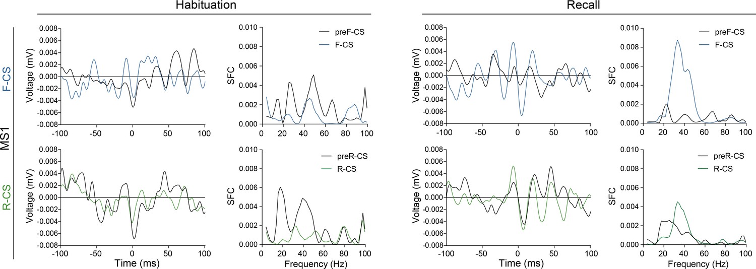
The aIC–pIC hierarchy is valence-asymmetric.

Valence-resolved STA of 200 ms pIC LFP traces centered around the occurrence of spikes from aIC and the resulting pIC LFP power-normalized SFC thereof for habituation and recall for animal MS1 (as in Figure 3B).

Figure 3—figure supplement 2

Download asset Open asset

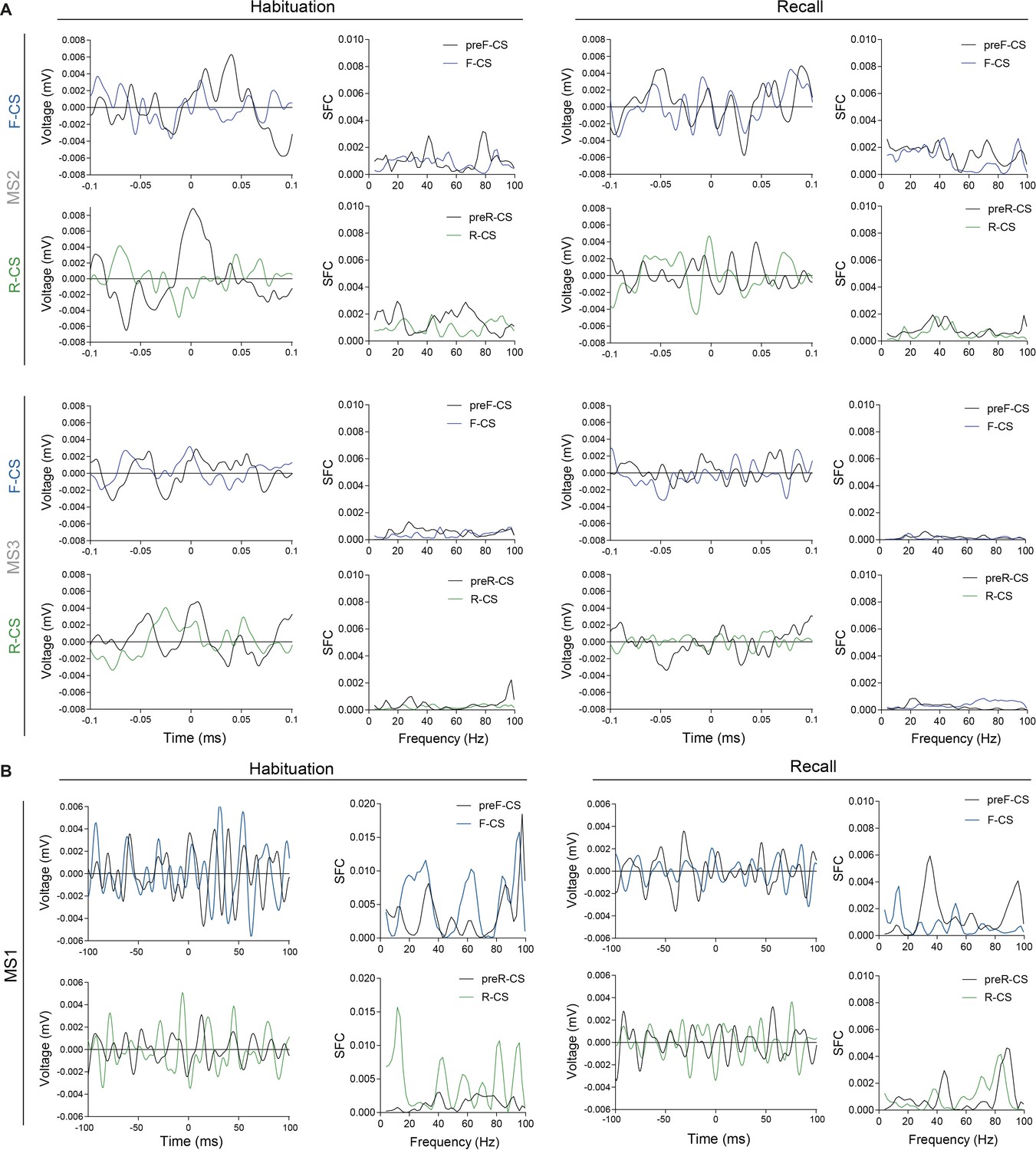
The aIC–pIC hierarchy is direction-asymmetric and performance-dependent.

(A) Valence-resolved STA of 200 ms pIC LFP traces centered around the occurrence of spikes from aIC and the resulting pIC LFP power-normalized SFC thereof for habituation and recall for worse-performing animals (MS2 and MS3 in Figure 1—figure supplement 8A). (B) Valence-resolved STA of 200 ms aIC LFP periods centered around the occurrence of spikes from pIC and the resulting aIC LFP power-normalized SFC thereof for habituation and recall for animal MS1 (as in Figure 3B).

Figure 4 with 3 supplements

Download asset Open asset

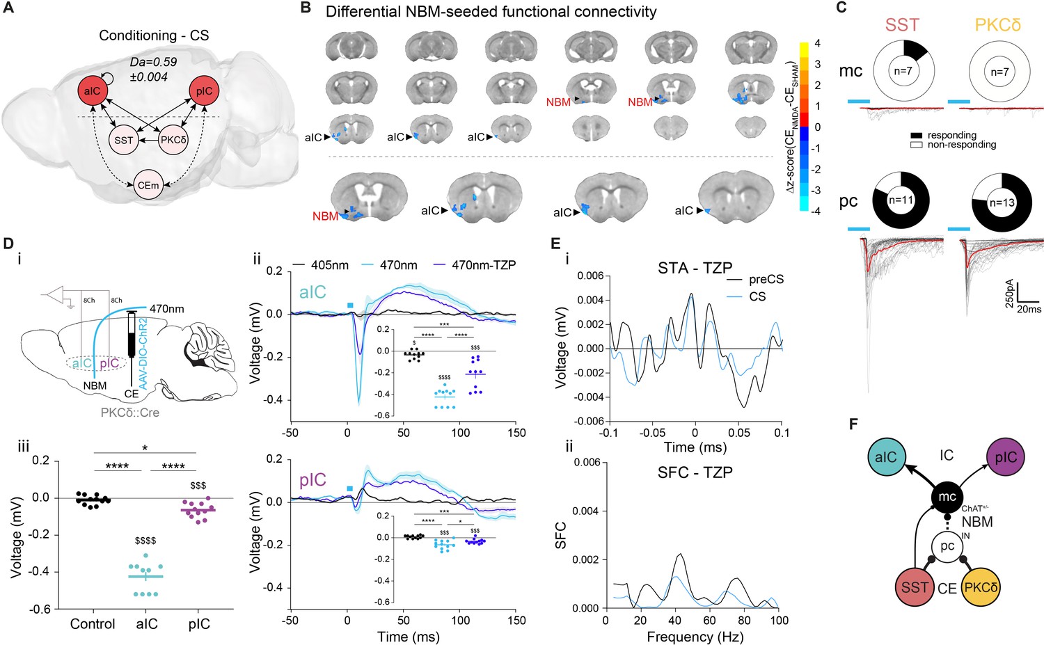
Basal forebrain NBM mediates bottom-up recruitment of IC activity.

(A) (i) Network depicting significant TE during CSs generated from data acquired from RC and FC stages. RF decoder accuracy (Da) for decoding CSs at RC and FC stages shown above network. Node color corresponds to feature importance from RF classification (Figure 2—figure supplement 2Aiii). (B) Chronic CE_NMDA reduced NBM resting-state functional connectivity to the right aIC compared to the CE_SHAM group. Two-sample t-test between CE_SHAM (n = 4) and CE_NMDA (n = 3) groups, followed by Gaussian Random Field Theory Multiple Comparison Correction (voxel-level p-value=0.05, cluster-level p-value=0.05). Differential z-score between CE_NMDA and CE_SHAM indicates depleted correlation (blue). (C) Fraction of magnocellular (mc)/parvocellular (pc) neurons in the NBM that responded with IPSCs upon optogenetic stimulation of CE^SST or CE^PKCδ input. (D) (i) In vivo optogenetic stimulation of the right CE^PKCδ–NBM pathway in two IC multi-site recorded, freely moving animals. (ii) Peri-laser stimulus time histograms of aIC (top) and pIC (bottom) channel-averaged LFP traces averaged over 60 (405, 470 nm) and 40 (470 nm-TZP) laser pulses. Traces represent averages of all available channels in aIC (11Ch) and pIC (12Ch). Insets depict respective minima of LFP traces within 20 ms after laser pulse onset. Significant one-way RM ANOVA for aIC (F_1,116,11,16=153.00, p<0.0001) and pIC (F_1,340,14,74=23.60, p<0.0001). (iii) Quantification of IC LFP minima upon CE^PKCδ–NBM stimulation under control conditions. Significant one-way ANOVA (F_2,32=209.40, p<0.0001). All data presented as mean ± SEM. Holm-Sidak post hoc analysis was used for comparison between treatments/regions (*) and one-sample t-test for individual differences to zero ($), */$p<0.05, ***/$$$p<0.001, ****/$$$$p<0.0001. Full statistical report in Appendix 1—table 1. (E) (i) STA from the recall stage of 200 ms pIC LFP traces centered around aIC spikes after systemic administration of TZP. (ii) SFC resulting from pIC LFP power-normalized STA from (i). (F) Circuit model of the bottom-up IC↔CE/NBM pathway consistent with experimental data. Dotted line represents a connection not assessed, but consistent with previous studies (Jolkkonen et al., 2002; Kapp et al., 1994).

Figure 4—source data 1 IC LFP responses upon optogenetic CE^PKCδ–NBM stimulation.: https://cdn.elifesciences.org/articles/60336/elife-60336-fig4-data1-v1.xlsx
Download elife-60336-fig4-data1-v1.xlsx

Figure 4—figure supplement 1

Download asset Open asset

ROI-based functional connectivity of the CE lesion group.

(A) (*top*) Mice received a bilateral injection of NMDA (N-methyl-D-aspartate, CE_NMDA, n = 3) or saline (CE_SHAM, n = 4, Figure 1A and see Figure 1—figure supplement 1) into CE. (*bottom*) Representative staining with NeuN from a mouse from the CE_NMDA group. scalebar = 100 µm. BLA – basolateral amygdala, Pir – piriform cortex. (B) Functional connectivity in the CE_NMDA group with significant (one sample t-test, p<0.05) Fisher z-transformed Pearson correlation coefficients between each pair of brain regions (blue-to-red scale) are shown (significance of correlations reflected by the size of the square). (C) Seed region mask used for functional connectivity of the NBM in Figure 4B.

Figure 4—figure supplement 1—source data 1 fMRI cross-correlation matrix of CE_NMDA in Figure 4—figure supplement 1B.: https://cdn.elifesciences.org/articles/60336/elife-60336-fig4-figsupp1-data1-v1.xlsx
Download elife-60336-fig4-figsupp1-data1-v1.xlsx

Figure 4—figure supplement 2

Download asset Open asset

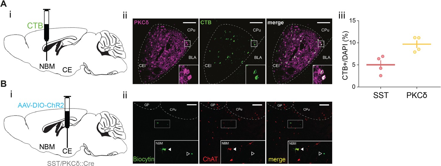
Anatomical and functional assessment of CE–NBM connectivity.

(A) (i) Schematic of stereotactic injection of CTB into the NBM with (ii) exemplary backlabeling in CE (red) and PKCδ counterstain (magenta) and (iii) quantification according to identified CEl populations. Each data point represents a single animal. (B) (i) To assess synaptic connectivity between CEl subpopulations and NBM shown in Figure 4C, SST::Cre and PKCδ::Cre mice received injections of an AAV carrying Cre-dependent DIO-ChR2 in the CE. (ii) Representative slice showing biocytin-filled and fluorescently labelled streptavidin-stained patched neurons (green) and immunolabeled ChAT⁺ neurons (red) in NBM. Arrows indicate exemplary magnocellular (mc, filled) and parvocellular neurons (pv, hollow).

Figure 4—figure supplement 3

Download asset Open asset

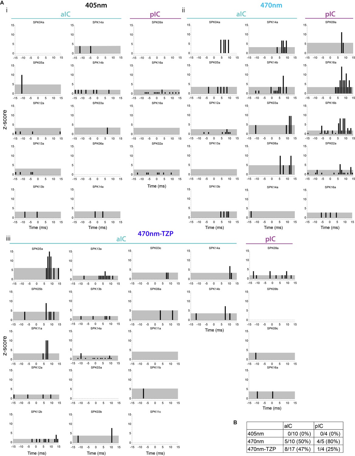
Optogenetic CE–NBM stimulation increases spiking of single neurons in aIC and pIC.

(A) Peri-laser stimulus time histograms of single unit activity in aIC and pIC upon the (i) control stimulus (405 nm, 60 5 ms pulses), (ii) CE^PKCδ-NBM stimulation (470 nm, 60 5 ms pulses) and (iii) CE^PKCδ-NBM stimulation after systemic administration of TZP (470 nm-TZP, 40 5 ms pulses). Gray area indicates 95% confidence interval (CI). (B) Summary table of responding neurons above 95% CI after laser stimulation.

Figure 5 with 6 supplements

Download asset Open asset

The CE–NBM pathway promotes top-down information for Pavlovian learning.

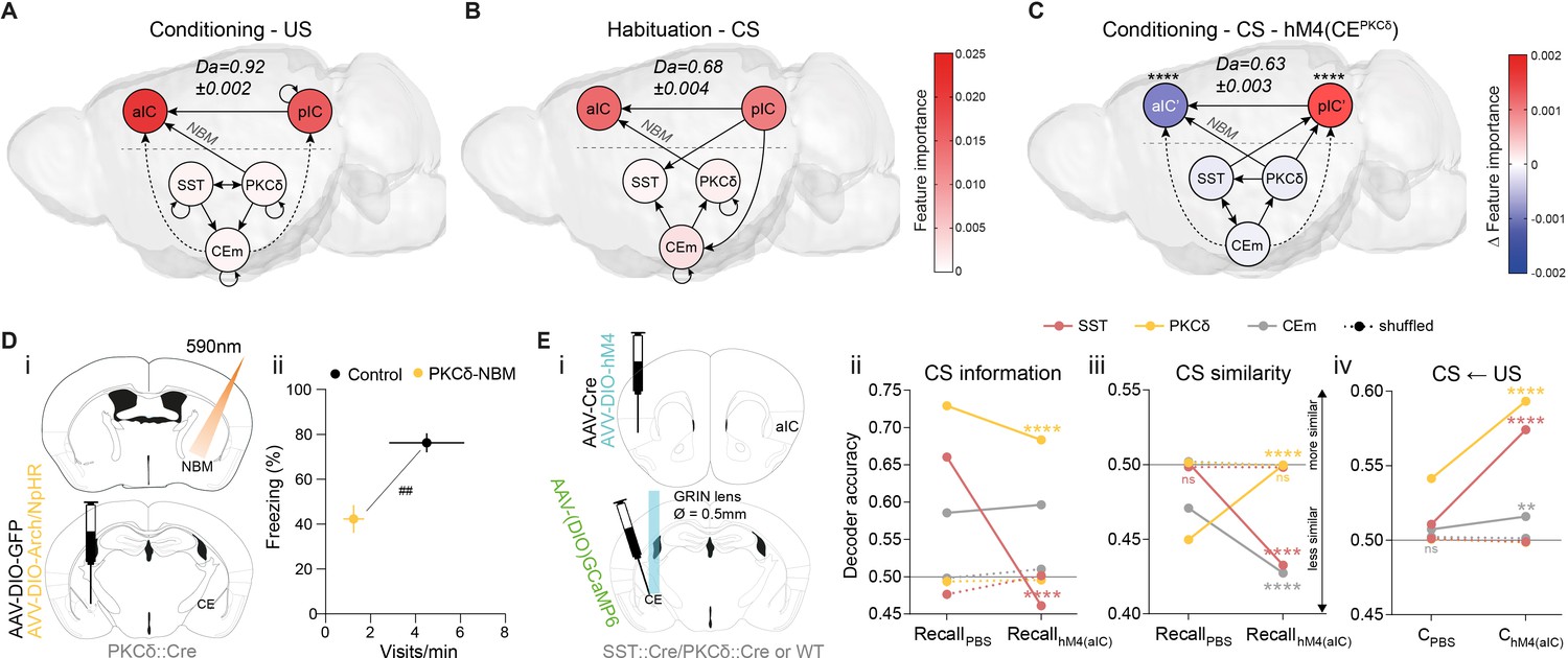
(A) Network depicting significant TE after US; generated from data acquired from RC and FC. RF decoder accuracy (Da) for decoding USs at RC and FC stages shown above network. Node color corresponds to feature importance resulting from RF classification under control conditions (see Figure 2—figure supplement 2Aiv). (B) Network depicting significant TE during CS in the habituation stage. RF Da for decoding CSs at habituation. Nodes are colored according to the feature importance resulting from RF classification (see Figure 2—figure supplement 2Av). (C) Network depicting significant TE during CS generated from data acquired during RC and FC. aIC/pIC data has been replaced by a dataset recorded during chemogenetic inhibition of CE^PKCδ (aIC’, pIC’) in the same animals (hM4(CE^PKCδ)). RF Da for decoding CSs at RC and FC stages during hM4(CE^PKCδ) shown above network. Feature importance given as differential from control conditions, with * indicating significant differences (see Figure 2—figure supplement 2Aiii). (D) (i) Experimental approach for optogenetic inhibition of the CE^PKCδ-NBM pathway during CS presentations at conditioning. (ii) Quantification of approach and avoidance behavior at recall (n_GFP = 7, n_{CE-PKCδ–NBM}=6; significant MANOVA, F_1,10=9.76, p=0.0045). Data presented as mean ± SEM. Holm post hoc as difference to control, ##p<0.01. (E) (i) Scheme for chemogenetic inhibition of aIC (hM4(aIC)) during CE population recordings. (ii) Mean CS Da of an MLP trained to detect CS information in the activity of 20 CE^SST, 30 CE^PKCδ, and 10 CEm best neurons per treatment to detect CS information at recall during control conditions (PBS) and hM4(aIC) (significant treatment x population interaction in a two-way ANOVA, F_5,4788=117.50, p<0.0001). (iii) Mean CS Da of an MLP trained on the activity of 20 CE^SST, 30 CE^PKCδ, and 10 CEm best neurons per treatment to detect R(F)-CS applied on F(R)-CS at recall during control conditions (PBS) and hM4(aIC) (significant treatment x population interaction in a two-way ANOVA, F_5,9588=306.50). (iv) Mean CS Da of an MLP trained on the activity of 20 CE^SST, 30 CE^PKCδ, and 10 CEm best neurons to detect R-US or F-US applied on R-CS or F-CS, respectively, in the conditioning stages during control conditions (PBS) and hM4(aIC) (significant treatment x population interaction in a two-way ANOVA, F_5,9588=163.90, p<0.0001). * Indicates significant differences between treatments within population, as determined by Holm-Sidak post hoc analysis, ****p<0.0001. Only non-significant differences to shuffled data are explicitly indicated (‘ns’). Full statistical report in Appendix 1—table 1.

Figure 5—source data 1 Decoding accuracy of an MLP classifier on single neuron activity of CE populations. Bold rows indicate neurons used as ‘best neurons’ in Figure 5E and Figure 5—figure supplement 5.: https://cdn.elifesciences.org/articles/60336/elife-60336-fig5-data1-v1.xlsx
Download elife-60336-fig5-data1-v1.xlsx
Figure 5—source data 2 Approach and avoidance behavior during the optogenetic CE^PKCδ–NBM manipulation cohort during recall.: https://cdn.elifesciences.org/articles/60336/elife-60336-fig5-data2-v1.xlsx
Download elife-60336-fig5-data2-v1.xlsx

Figure 5—figure supplement 1

Download asset Open asset

Supporting RF data and TE maps.

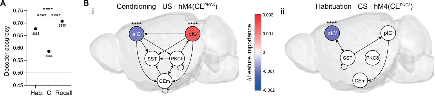
(A) RF Da for decoding CS under control conditions in the respective stages (one-way ANOVA, F_2,5997=271.60, p<0.0001). Holm-Sidak post hoc for all analyses, ****/$$$$ p<0.0001, * Indicates a significant difference as determined by two-sample t-tests, $ indicates a significant difference as determined by one-sample t-tests to random (0.5). Full statistical report in Appendix 1—table 1. (B) TE networks for (i) US in conditioning and (ii) CS in habituation under the hM4(CE^PKCδ) condition. Node color corresponds to feature importance from RF decoding shown in Figure 2—figure supplement 2Aiv and v, respectively.

Figure 5—figure supplement 2

Download asset Open asset

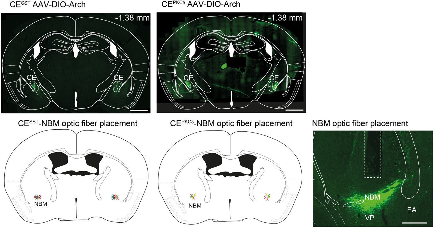
Histological verification of the optogenetic CE–NBM manipulation cohorts.

CE^SST and CE^PKCδ injection sites of AAV-DIO-Arch/NpHR3.0-YFP (scalebar = 900 µm) (*top*) and optic fiber placement in NBM (scalebar = 100 µm) (*bottom*). Schematic placement of the optic fiber tip above the terminal field in NBM marked with ‘x’ (*bottom, right*).

Figure 5—figure supplement 3

Download asset Open asset

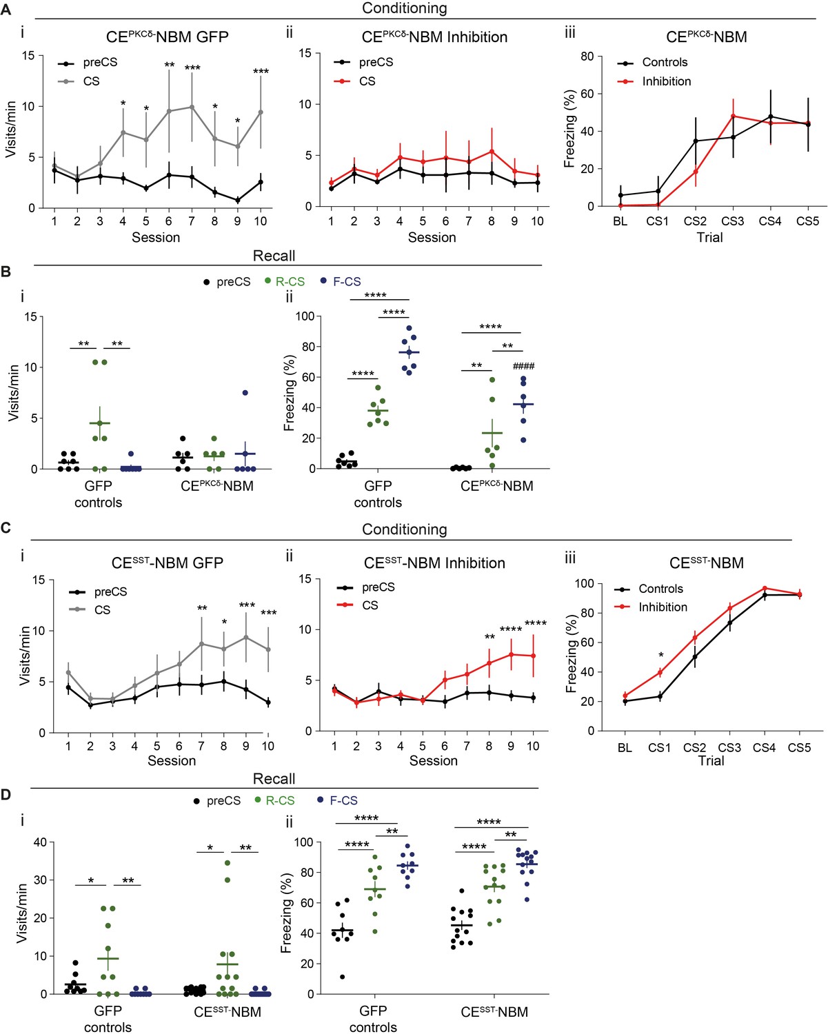
A cell-type-specific CE–NBM pathway is required for Pavlovian learning.

(A) Learning curves of approach behavior of the CE^PKCδ-NBM cohort in (i) controls (significant CS x session interaction in a two-way RM ANOVA, F_9,54=2.54, p=0.0163) and (ii) the CE^PKCδ-NBM inhibition group (no significant effect in a two-way RM ANOVA). (iii) Learning curves for avoidance behavior in the control and CE^PKCδ-NBM inhibition group during the FC stage (significant effect of trial in a two-way RM ANOVA, F_5,60=15.37, p<0.0001). (B) Quantification of CS-specific (i) approach (visits/min)(significant CS x treatment interaction in a two-way RM ANOVA, F_2,22=3.97, p=0.0338) and (ii) avoidance behavior (percent time spent freezing) (significant CS x treatment interaction in a two-way RM ANOVA, F_2,22=3.11, p=0.0095) at the recall session. ##p<0.01 (compared to control group), **/##p<0.01, ****p<0.0001; n_GFP = 7, n_{CE-PKCδ–NBM}=6, Data presented as mean ± SEM. (C) Learning curves of approach behavior for the CE^SST-NBM cohort in (i) controls (significant CS x session interaction in a two-way RM ANOVA, F_9,72=2.63, p=0.0109) and (ii) the CE^SST-NBM inhibition group (significant CS x session interaction in a two-way RM ANOVA, F_9,108=4.75, p<0.0001). (iii) Learning curves for avoidance behavior of the control and CE^SST-NBM inhibition groups during the FC stage (significant effect of treatment in a two-way RM ANOVA, F_1,20=10.70, p=0.0038). (D) Quantification of CS-specific (i) approach (significant effect of CS in a two-way RM ANOVA, F_2,40=11.59, p=0.0001) and (ii) avoidance behavior (significant effect of CS in a two-way RM ANOVA, F_2,40=77.68, p<0.0001) at recall for the CE^SST-NBM cohort. Holm-Sidak post hoc for all analyses, *p<0.05, **p<0.01, ***p<0.001, ****p<0.0001. n_GFP = 9, n_CE-SST–NBM=13. All data presented as mean ± SEM. Full statistical report in Appendix 1—table 1.

Figure 5—figure supplement 4

Download asset Open asset

Histology of hM4 expression in calcium imaging cohorts.

Injection site of AAV-DIO-hM4-mCherry and AAV::Cre into aIC. Scalebar = 200 µm. AIC – agranular insula, Cl – claustrum, G/DIC – granular/dysgranular insula, Pir – piriform cortex, rf – rhinal fissure.

Figure 5—figure supplement 5

Download asset Open asset

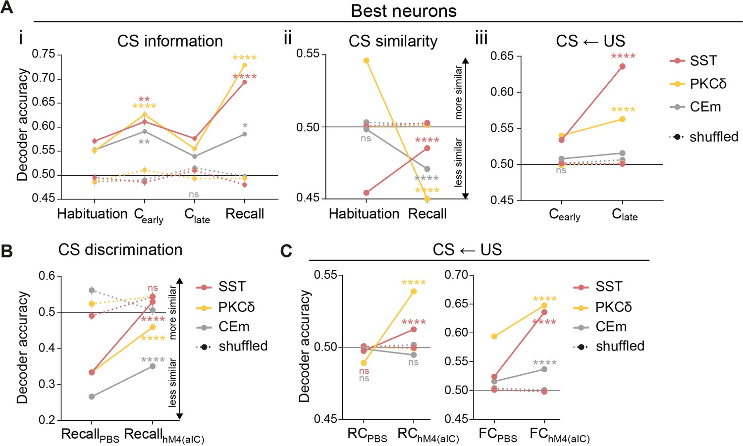
Valence-specific mapping of CS and US features in IC–CE circuitry.

(A) Same decoding approach as in Figure 1D, using best neurons (see ‘Single-region decoding’ in Materials and methods) for (i) CS information (significant stage x population interaction in a two-way ANOVA, F_15,9576=34.91, p<0.0001), (ii) CS similarity (significant stage x population interaction in a two-way ANOVA, F_5,9588=311.70, p<0.0001) and (iii) the CS←US task (significant stage x population interaction in a two-way ANOVA, F_5,9588=163.90, p<0.0001). (B) Alternative decoding approach for CS discrimination (as in Figure 1—figure supplement 7B), using best neurons in control conditions (PBS) and aIC inhibition (hM4(aIC)) at recall (significant treatment x population interaction in a two-way ANOVA, F_5,2387=29.37, p<0.0001). (C) Projection of US properties by application of an MLP trained to detect US information in best neurons of CE populations under control conditions (PBS) and aIC inhibition (hM4(aIC)), applied to the respective CS (RC: significant treatment x population interaction in a two-way ANOVA, F_5,4788=186.13, p<0.0001; FC: significant treatment x population interaction in a two-way ANOVA, F_5,4788=195.10, p<0.0001). * Indicates significant differences between stages, within population. Holm-Sidak post hoc for all analyses, *p<0.05, **p<0.01, ***p<0.001, ****/####p<0.0001. All data presented as mean ± SEM. Full statistical report in Appendix 1—table 1.

Figure 5—figure supplement 6

Download asset Open asset

Hierarchical interactions in IC↔CE/NBM circuitry.

(*Left*) Stimulus salience at the lower hierarchical level in the amygdala promotes interoceptive models from the IC via CE^PKCδ when uncertain about value. In the absence of interoceptive value in CE CS salience engages NBM-aIC interaction to update intra-insular models. (*Right*) Insular interoceptive models about stimulus values are recruited by CE and segregate into salience and valence dimensions, which are differentially projected onto CE microcircuitry.

Tables

Key resources table

Reagent type (species) or resource	Designation	Source or reference	Identifiers	Additional information
Strain, strain background (M. musculus, male)	wild-type	Charles River Laboratories		C57BL/6J background
Strain, strain background (M. musculus, male)	PKCδ::Cre	doi:10.1038/nature09553	Prkcd::GluClα::Cre	C57BL/6J background
Strain, strain background (M. musculus, male)	SST::Cre	Jackson Laboratory	SOM-IRES::Cre; stock no: 013044	C57BL/6J background
Other	DIO-GFP	This paper	AAV5.EF1a.DIO.GFP.WPRE	AAV vectors to transduce brain tissue; Titer:9.73E+10
Other	syn-GFP	Penn Vector Core	AAV5.hsyn.eGFP.WPRE	AAV vectors to transduce brain tissue; Titer:1.15E+13
Other	syn-ChR2	Penn Vector Core	AAV5.hsyn.hChR2(H134R).eYFP.WPRE	AAV vectors to transduce brain tissue; Titer:1.87E+13
Other	DIO-ChR2	Penn Vector Core	AAV5.EF1a.DIO.hChR2(H134R).eYFP.WPRE	AAV vectors to transduce brain tissue; Titer:1.30E+13
Other	syn-Arch	Penn Vector Core	AAV5.hsyn.ArchT.YFP.WPRE	AAV vectors to transduce brain tissue; Titer:4.68E+12
Other	DIO-Arch	BI Biberach	AAV5. Ef1a.DIO.eArch.eYFP.WPRE	AAV vectors to transduce brain tissue; Titer:6.00E+12
Other	DIO-NpHR	Penn Vector Core	AAV5.Ef1a.DIO.eNpHR3.0-eYFP.WPRE	AAV vectors to transduce brain tissue; Titer:2.59E+12
Other	GCaMP6m	BI Biberach	AAV9.hsyn.GCaMP6m.WPRE	AAV vectors to transduce brain tissue; Titer:1.00E+12
Other	DIO-GCaMP6f	Penn Vector Core	AAV1.hsyn.DIO.GCaMP6f.WPRE.	AAV vectors to transduce brain tissue; Titer:1.00E+13
Other	AAV::Cre	Vector Biolabs	AAV5.CMV.Cre	AAV vectors to transduce brain tissue; Titer:1.00E+12
Other	CAV::Cre	Montpellier Vector Platform	CAV2.Cre	CAV vectors to transduce brain tissue; Titer:5.50E+12
Other	DIO-hM4	Penn Vector Core	AAV5.hsyn.DIO.hM4D.mCherry.WPRE	AAV vectors to transduce brain tissue; Titer:1.01E+13
Chemical compound, drug	DAPI	Life technologies	DAPI	1 µg/mL
Chemical compound, drug	TZP	Sigma	CAS #147416-96-4	(3 mg/kg)
Antibody	Anti-PKCδ (mouse monoclonal)	BD Biosciences	Cat. #610398	Lot#4080743 IF(1:1000)
Antibody	Anti-FOXO3/NeuN (chicken polyclonal)	Abcam	Cat. #ab131624	Lot#GR88877-12 – IF(1:500)
Antibody	Anti-ChAT (goat polyclonal)	Millipore	Cat. #AB144P	Lot#2280814 – IF(1:200)
Antibody	Anti-mouse (goat polyclonal)	Life technologies	Cat. #A21052	Lot#1712097 – IF(1:1000)
Antibody	Anti-chicken (goat polyclonal)	Life technologies	Cat. #A11041	Lot#1383072 – (1:1000)
Antibody	Anti-goat (donkey polyclonal)	Abcam	Cat. #A11057	Lot#819578 – IF(1:500)
Peptide, recombinant protein	Streptavidin-Alexa Fluor	Life technologies	Cat. #S11223	Lot#18585036 – IF(1:1000)
Peptide, recombinant protein	CTB-Alexa Fluor	Invitrogen	Cat. #C34775
Software, algorithm	GraphPad Prism 7 and 8	GraphPad Software, Inc	Version 8.1.1
Software, algorithm	scikit-learn package	doi:10.1007/s13398-014-0173-7.2	Python 3

Appendix 1—table 1

Detailed statistical report for MANOVA/ANOVA analyses.

Dataset	Statistical test	p-values	F ratio (DFn, DFd)
Figure 1Ci CS IC Stage x Subregion Stage Subregion	Two-way ANOVA	p<0.0001 p<0.0001 p<0.0001	F_9,6384=13.69 F_3,6384=29.11 F_3,6384=203.31
Figure 1Cii CS similarity IC Stage x Subregion Stage Subregion	Two-way ANOVA	p<0.0001 p<0.0001 p<0.0001	F_3,6392=42.10 F_{1, 6392}=116.62 F_{3, 6392}=42.69
Figure 1Cii CS←US transfer IC Stage x Subregion Stage Subregion	Two-way ANOVA	p<0.0001 p<0.0001 p<0.0001	F_3,6392=50.14 F_1,6392=102.10 F_3,6392=469.13
Figure 1Di CS CE Stage x Population Stage Population	Two-way ANOVA	p<0.0001 p<0.0001 p<0.0001	F_15,9576=9.30 F_3,9576=30.92 F_5,9576=28.20
Figure 1Dii CS similarity CE Stage x Population Stage Population	Two-way ANOVA	p<0.0001 p<0.0001 p<0.0001	F_5,9588=30.40 F_1,9588=25.90 F_5,9588=33.87
Figure 1Diii CS←US transfer CE Stage x Population Stage Population	Two-way ANOVA	p<0.0001 p<0.0001 p<0.0001	F_5,9588=339.60 F_1,9588=88.70 F_5,9588=798.90
Figure 2Dii Conditioning early	MANOVA	p=0.0126	F_2,44=3.60
Figure 2Dii Conditioning late	MANOVA	p=0.0004	F_2,44=6.43
Figure 2Diii, left Recall opto	MANOVA	p=0.0050	F_1,13=8.18
Figure 2Diii, right Recall hM4(pIC)	MANOVA	p=0.0067	F_1,17=6.81
Figure 3Cii Recall hM4(aIC)-pIC	MANOVA	p=0.0471	F_1,18=3.64
Figure 4Dii CE^PKCδ-NBM stim. aIC pIC	One-way RM ANOVA	p<0.0001 p<0.0001	F_1,116,11,16=153.00 F_1,340,14,74=23.60
Figure 4Diii CE^PKCδ-NBM stim.	One-way ANOVA	p<0.0001	F_2,32=209.40
Figure 5Dii Recall CE^PKCδ-NBM	MANOVA	p=0.0045	F_1,10=9.76
Figure 5Eii CS CE Treatment x Population Treatment Population	Two-way ANOVA	p<0.0001 p<0.0001 p<0.0001	F_5,4788=117.50 F_1,4788=102.80 F_5,4788=449.30
Figure 5Eiii CS similarity CE Treatment x Population Treatment Population	Two-way ANOVA	p<0.0001 p<0.0001 p<0.0001	F_5,9588=306.50 F_1,9588=134.80 F_5,9588=340.70
Figure 5Eiv CS←US transfer CE Treatment x Population Treatment Population	Two-way ANOVA	p<0.0001 p<0.0001 p<0.0001	F_5,9588=163.90 F_1,9588=432.50 F_5,9588=584.50
Figure 1—figure supplement 5Ai Habituation R-CS Time x Subregion Time Subregion	Two-way RM ANOVA	p=0.1764 p=0.0037 p=0.7836	F_52,11180=1.18 F_52,11180=1.61 F_1,215=0.08
Figure 1—figure supplement 5Ai Habituation F-CS Time x Subregion Time Subregion	Two-way RM ANOVA	p<0.0001 p<0.0001 p=0.9293	F_52,11076=2.23 F_52,11076=2.17 F_1,213=0.008
Figure 1—figure supplement 5Aiii Habituation R-CS Responders Time x Subregion Time Subregion	Two-way RM ANOVA	p=0.8104 p<0.0001 p=0.6977	F_52,1664=0.82 F_52,1664=5.682 F_1,32=0.1536
Figure 1—figure supplement 5Aiii Habituation F-CS Responders Time x Subregion Time Subregion	Two-way RM ANOVA	p=0.0007 p<0.0001 p=0.7154	F_52,884=1.782 F_52,884=2.497 F_1,17=0.1374
Figure 1—figure supplement 5Bii R-US Time x Subregion Time Subregion	Two-way RM ANOVA	p=0.0002 p=0.9740 p=0.0021	F_52,14248=1.87 F_52,14248=0.66 F_1,274=9.62
Figure 1—figure supplement 5Biv F-US Time x Subregion Time Subregion	Two-way RM ANOVA	p<0.0001 p<0.0001 p=0.0587	F_50,7100=2.29 F_50,7100=5.03 F_1,142=3.63
Figure 1—figure supplement 5Ci Recall R-CS Time x Subregion Time Subregion	Two-way RM ANOVA	p=0.0537 p=0.1030 p=0.79	F_52,14560=1.34 F_52,14560=1.26 F_1,280=0.07
Figure 1—figure supplement 5Ci Recall F-CS Time x Subregion Time Subregion	Two-way RM ANOVA	p=0.5919 p<0.0001 p=0.3279	F_52,14560=0.94 F_52,14560=2.42 F_1,280=0.961
Figure 1—figure supplement 5Ciii Recall R-CS Responders Time x Subregion Time Subregion	Two-way RM ANOVA	p=0.1447 p<0.0001 p=0.1309	F_52,1924=1.212 F_52,1924=2.984 F_1,37=2.387
Figure 1—figure supplement 5Ciii Recall F-CS Responders Time x Subregion Time Subregion	Two-way RM ANOVA	p<0.0001 p<0.0001 p=0.4025	F_52,1716=2.159 F_52,1716=6.107 F_1,33=0.7194
Figure 1—figure supplement 6Ai Habituation R-CS Time x Population Time Population	Two-way RM ANOVA	p<0.0001 p=0.1186 p=0.9656	F_64,3232=2.76 F_32,3232=1.30 F_2,101=0.036
Figure 1—figure supplement 6Ai Habituation F-CS Stage x Population Stage Population	Two-way RM ANOVA	p<0.0001 p=0.0104 p=0.1205	F_64,4032=2.43 F_32,4032=1.67 F_2,126=2.15
Figure 1—figure supplement 6Aiii Habituation R-CS Responders Time x Population Time Subregion	Two-way RM ANOVA	p=0.9238 p<0.0001 p=0.9813	F_64,800=0.7528 F_32,800=7.436 F_2,25=0.0189
Figure 1—figure supplement 6Aiii Habituation F-CS Responders Time x Population Time Subregion	Two-way RM ANOVA	p=0.0005 p<0.0001 p=0.0473	F_64,1056=1.721 F_32,1056=2.425 F_2,33=3.353
Figure 1—figure supplement 6Bii R-US Time x Population Time Population	Two-way RM ANOVA	p<0.0001 p<0.0001 p<0.0001	F_56,3976=2.45 F_28,3976=9.61 F_2,142=11.18
Figure 1—figure supplement 6Biv F-US Time x Population Time Population	Two-way RM ANOVA	p<0.0001 p<0.0001 p=0.6376	F_56,4480=4.22 F_28,4480=31.28 F_2,160=0.451
Figure 1—figure supplement 6Ci Recall R-CS Time x Population Time Population	Two-way RM ANOVA	p<0.0001 p=0.5507 p=0.8385	F_72,9684=2.81 F_36,9684=0.952 F_2,269=0.176
Figure 1—figure supplement 6Ci Recall F-CS Time x Population Time Population	Two-way RM ANOVA	p<0.0001 p<0.0001 p=0.2932	F_72,9072=2.01 F_36,9072=9.42 F_2,252=1.23
Figure 1—figure supplement 6Ciii Recall R-CS Responders Time x Population Time Population	Two-way RM ANOVA	p<0.0001 p<0.0001 p=0.6363	F_72,2952=3.577 F_36,2952=16.4 F_2,82=0.4546
Figure 1—figure supplement 6Ciii Recall F-CS Responders Time x Population Time Subregion	Two-way RM ANOVA	p<0.0001 p<0.0001 p=0.4251	F_72,3240=2.273 F_52,3240=28.5 F₂,₉₀=0.8636
Figure 1—figure supplement 7Ai R-CS IC Stage x Subregion Stage Subregion	Two-way ANOVA	p<0.0001 p<0.0001 p<0.0001	F_9,3184=5.68 F_3,3184=9.99 F_3,3184=78.65
Figure 1—figure supplement 7Aii F-CS IC Stage x Subregion Stage Subregion	Two-way ANOVA	p<0.0001 p<0.0001 p<0.0001	F_9,3184=11.50 F_3,3184=22.38 F_3,3184=137.80
Figure 1—figure supplement 7Aiii R-CS CE Stage x Population Stage Population	Two-way ANOVA	p<0.0001 p<0.0001 p<0.0001	F_15,4776=29.17 F_3,4776=23.21 F_5,4776=28.00
Figure 1—figure supplement 7Aiv F-CS CE Stage x Population Stage Population	Two-way ANOVA	p<0.0001 p<0.0001 p<0.0001	F_15,4776=7.93 F_3,4776=13.56 F_5,4776=24.62
Figure 1—figure supplement 7Bi CS discrimination IC Stage x Subregion Stage Subregion	Two-way ANOVA	p<0.0001 p<0.0001 p<0.0001	F_3,1592=18.53 F_1,1592=27.94 F_3,1592=479.8
Figure 1—figure supplement 7Bii CS discrimination CE Stage x Population Stage Population	Two-way ANOVA	p<0.0001 p<0.0001 p<0.0001	F_5,2366=15.58 F_1,2366=19.37 F_5,2366=25.30
Figure 1—figure supplement 7Ci R-US IC Stage x Subregion Stage Subregion	Two-way ANOVA	p<0.0001 p=0.0030 p<0.0001	F_3,1592=16.06 F_1,1592=8.85 F_3,1592=302.70
Figure 1—figure supplement 7Ci F-US IC Stage x Subregion Stage Subregion	Two-way ANOVA	p=0.2300 p=0.8792 p<0.0001	F_3,1592=1.44 F_1,1592=0.02 F_3,1592=1619.00
Figure 1—figure supplement 7Ci R-US CE Stage x Population Stage Subregion	Two-way ANOVA	p<0.0001 p=0.0213 p<0.0001	F_5,2228=5.40 F_1,2228=5.31 F_5,2228=23.34
Figure 1—figure supplement 7Ci F-US CE Stage x Population Stage Subregion	Two-way ANOVA	p=0.0013 p=0.0020 p<0.0001	F_5,2388=4.01 F_1,2388=9.53 F_5,2388=76.81
Figure 1—figure supplement 7Cii RC CS←US transfer IC Stage x Subregion Stage Subregion	Two-way ANOVA	p<0.0001 p<0.0001 p<0.0001	F_9,3192=242.50 F_3,3192=521.60 F_3,3192=167.50
Figure 1—figure supplement 7Cii FC CS←US transfer IC Stage x Subregion Stage Subregion	Two-way ANOVA	p<0.0001 p<0.0001 p<0.0001	F_9,3192=9.97 F_3,3192=11.62 F_3,3192=688.50
Figure 1—figure supplement 7Cii RC CS←US transfer CE Stage x Population Stage Population	Two-way ANOVA	p<0.0001 p=0.0013 p<0.0001	F_5,4788=18.39 F_1,4788=10.42 F_5,4788=326.10
Figure 1—figure supplement 7Cii FC CS←US transfer CE Stage x Population Stage Population	Two-way ANOVA	p<0.0001 p<0.0001 p<0.0001	F_5,4788=603.30 F_1,4788=142.20 F_5,4788=1057.40
Figure 1—figure supplement 8Bi aIC R-US Time x Performance Time Performance	Two-way RM ANOVA	p=0.0029 p=0.0034 p=0.0388	F_52,7592=1.63 F_52,7592=1.62 F_1,146=4.35
Figure 1—figure supplement 8Bii aIC F-US Time x Performance Time Performance	Two-way RM ANOVA	p<0.0001 p<0.0001 p=0.9474	F_50,3950=2.47 F_50,3950=2.50 F_1,79=0.004
Figure 1—figure supplement 8Biii pIC R-US Time x Performance Time Performance	Two-way RM ANOVA	p<0.0001 p<0.0001 p=0.6200	F_52,6552=9.86 F_52,6552=3.55 F_1,126=0.247
Figure 1—figure supplement 8Biv pIC F-US Time x Performance Time Performance	Two-way RM ANOVA	p<0.0001 p<0.0001 p<0.0001	F_50,3050=3.27 F_50,3050=5.93 F_1,61=17.59
Figure 1—figure supplement 8Ci aIC R-CS Time x Performance Time Performance	Two-way RM ANOVA	p<0.0001 p=0.6431 p=0.5547	F_52,8268=2.09 F_52,8268=0.917 F_1,159=0.350
Figure 1—figure supplement 8Cii aIC F-CS Time x Performance Time Performance	Two-way RM ANOVA	p=0.0434 p=0.0002 p=0.8521	F_52,8268=1.36 F_52,8268=1.84 F_1,159=0.0349
Figure 1—figure supplement 8Ciii pIC R-CS Time x Performance Time Performance	Two-way RM ANOVA	p>0.9999 p=0.1204 p=0.8266	F_52,6188=0.353 F_52,6188=1.24 F_1,119=0.05
Figure 1—figure supplement 8Civ pIC F-CS Time x Performance Time Performance	Two-way RM ANOVA	p=0.0003 p=0.0063 p=0.3331	F_52,6188=1.81 F_52,6188=1.56 F_1,119=0.944
Figure 1—figure supplement 8Di SST R-US Time x Performance Time Performance	Two-way RM ANOVA	p<0.0001 p<0.0001 p=0.0607	F_28,3052=2.33 F_28,3052=2.49 F_1,109=3.59
Figure 1—figure supplement 8Dii SST water Time x Performance Time Performance	Two-way RM ANOVA	p=0.1217 p<0.0001 p=0.0187	F_28,3052=1.32 F_28,3052=20.42 F_1,109=5.70
Figure 1—figure supplement 8Diii SST F-US Time x Performance Time Performance	Two-way RM ANOVA	p=0.0003 p<0.0001 p=0.9986	F_28,1344=2.22 F_28,1344=8.10 F_1,48=3.012e-006
Figure 1—figure supplement 8Div PKCδ R-US Time x Performance Time Performance	Two-way RM ANOVA	p<0.0001 p=0.0342 p=0.7613	F_28,3192=3.07 F_28,3192=1.54 F_1,114=0.09
Figure 1—figure supplement 8Dv PKCδ water Time x Performance Time Performance	Two-way RM ANOVA	p=0.0262 p<0.0001 p=0.6868	F_28,3220=1.56 F_28,3220=2.67 F_1,115=0.16
Figure 1—figure supplement 8Dvi PKCδ F-US Time x Performance Time Performance	Two-way RM ANOVA	p<0.0001 p<0.0001 p=0.3513	F_28,1848=2.96 F_28,1848=6.32 F_1,66=0.88
Figure 1—figure supplement 8Dvii CEm R-US Time x Performance Time Performance	Two-way RM ANOVA	p>0.999 p<0.0001 p=0.7647	F_28,1512=0.18 F_28,1512=3.95 F_1,54=0.09
Figure 1—figure supplement 8Dviii CEm water Time x Performance Time Performance	Two-way RM ANOVA	p<0.0001 p<0.0001 p=0.5895	F_28,1512=2.92 F_28,1512=3.53 F_1,54=0.30
Figure 1—figure supplement 8Dix CEm F-US Time x Performance Time Performance	Two-way RM ANOVA	p=0.9646 p<0.0001 p=0.6271	F_28,1204=0.57 F_28,1204=22.73 F_1,43=0.24
Figure 2—figure supplement 2Ai Feature importance behavior	One-way ANOVA	p<0.0001	F_9,156190=5184.00
Figure 2—figure supplement 2Aii Feature importance CS	One-way ANOVA	p<0.0001	F_9,73454=2437.00
Figure 2—figure supplement 2Aiii Feature importance CS hM4 CE^PKCδ	One-way ANOVA	p<0.0001	F_9,77790=5185.00
Figure 2—figure supplement 2Aiv Feature importance US hM4 CE^PKCδ	One-way ANOVA	p<0.0001	F_9,77821=2126.00
Figure 2—figure supplement 2Av Feature importance habituation CS hM4 CE^PKCδ	One-way ANOVA	p<0.0001	F_9,77619=1766.00
Figure 2—figure supplement 5Ai RC port visits opto Session x Treatment Session Treatment	Two-way RM ANOVA	p<0.0001 p<0.0001 p=0.0271	F_14,154=3.40 F_7,154=15.39 F_2,22=4.27
Figure 2—figure supplement 5Aii FC freezing opto Treatment x Trial Treatment Trial	Two-way RM ANOVA	p<0.0001 p<0.0001 p=0.0054	F_10,110=4.71 F_5,110=50.67 F_2,22=6.69
Figure 2—figure supplement 5Bi Recall port visits opto CS x Treatment CS Treatment	Two-way RM ANOVA	p=0.2605 p<0.0001 p=0.0343	F_4,44=1.37 F_2,44=17.90 F_2,22=3.95
Figure 2—figure supplement 5Bii Recall freezing opto CS x Treatment CS Treatment	Two-way RM ANOVA	p=0.0225 p<0.0001 p=0.0154	F_4,44=3.17 F_2,44=66.66 F_2,22=5.07
Figure 2—figure supplement 7Ai RC GFP CS x Session CS Session	Two-way RM ANOVA	p<0.0001 p=0.0001 p<0.0001	F_13,130=5.97 F_1,10=38.23 F_13,130=4.64
Figure 2—figure supplement 7A ii RC hM4(pIC)-CE CS x Session CS Session	Two-way RM ANOVA	p<0.0001 p=0.0027 p<0.0001	F_13,91=9.07 F_1,7=20.62 F_13,91=8.09
Figure 2—figure supplement 7Aiii RC hM4(aIC)-pIC CS x Session CS Session	Two-way RM ANOVA	p=0.0003 p=0.0053 p<0.0001	F_13,104=3.30 F_1,8=14.36 F_13,104=4.86
Figure 2—figure supplement 7Aiv FC Treatment x Trial Treatment Trial	Two-way RM ANOVA	p=0.0537 p=0.56 p<0.0001	F_10,125=1.88 F_2,25=0.59 F_5,125=174.70
Figure 2—figure supplement 7B Recall port visits hM4(pIC)-CE CS x Treatment CS Treatment	Two-way RM ANOVA	p=0.9251 p<0.0001 p=0.7647	F_2,36=0.08 F_2,36=31.88 F_1,18=0.09
Figure 2—figure supplement 7B Recall freezing hM4(pIC)-CE CS x Treatment CS Treatment	Two-way RM ANOVA	p=0.2970 p<0.0001 p=0.0087	F_2,36=1.26 F_2,36=40.47 F_1,18=8.65
Figure 2—figure supplement 7B Recall port visits hM4(aIC)-pIC CS x Treatment CS Treatment	Two-way RM ANOVA	p=0.9652 p<0.0001 p=0.7341	F_2,38=0.04 F_2,38=30.32 F_1,19=0.19
Figure 2—figure supplement 7B Recall freezing hM4(aIC)-pIC CS x Treatment CS Treatment	Two-way RM ANOVA	p=0.4522 p<0.0001 p=0.0008	F_2,38=0.81 F_2,38=54.69 F_1,19=15.80
Figure 5—figure supplement 1A RF Da Control	One-way ANOVA	p<0.0001	F_2,5997=271.60
Figure 5—figure supplement 3Ai RC Control CS x Session CS Session	Two-way RM ANOVA	p=0.0163 p=0.0745 p=0.1830	F_9,54=2.54 F_1,6=4.65 F_9,54=1.47
Figure 5—figure supplement 3Aii RC CE^PKCδ-NBM CS x Session CS Session	Two-way RM ANOVA	p=0.9163 p=0.1080 p=0.5668	F_9,45=0.42 F_1,5=3.82 F_9,45=0.86
Figure 5—figure supplement 3Aiii FC freezing Trial x Treatment Trial Treatment	Two-way RM ANOVA	p=0.5363 p<0.0001 p=0.7568	F_5,60=0.83 F_5,60=15.37 F_1,12=0.10
Figure 5—figure supplement 3Bi Recall port visits CE^PKCδ-NBM CS x Treatment CS Treatment	Two-way RM ANOVA	p=0.0338 p=0.0434 p=0.5666	F_2,22=3.97 F_2,22=3.63 F_1,11=0.35
Figure 5—figure supplement 3Bii Recall freezing CE^PKCδ-NBM CS x Treatment CS Treatment	Two-way RM ANOVA	p=0.0095 p<0.0001 p=0.0029	F_2,22=3.11 F_2,22=81.45 F_1,11=8.72
Figure 5—figure supplement 3Ci RC Control CS x Session CS Session	Two-way RM ANOVA	p=0.0109 p=0.0104 p=0.0048	F_9,72=2.63 F_1,8=11.08 F_9,72=2.96
Figure 5—figure supplement 3Cii RC CE^SST-NBM CS x Session CS Session	Two-way RM ANOVA	p<0.0001 p=0.0062 p=0.0008	F_9,108=4.75 F_1,12=10.99 F_9,108=3.48
Figure 5—figure supplement 3Ciii FC freezing Trial x Treatment Trial Treatment	Two-way RM ANOVA	p=0.3490 p<0.0001 p=0.0038	F_5,100=1.13 F_5,100=119.10 F_1,20=10.70
Figure 5—figure supplement 3Di Recall port visits CE^SST-NBM CS x Treatment CS Treatment	Two-way RM ANOVA	p=0.9034 p=0.0001 p=0.5441	F_2,40=0.10 F_2,40=11.59 F_1,20=0.38
Figure 5—figure supplement 3Dii Recall freezing CE^SST-NBM CS x Treatment CS Treatment	Two-way RM ANOVA	p=0.9419 p<0.0001 p=0.5966	F_2,40=0.06 F_2,40=77.68 F _1,20=0.29
Figure 5—figure supplement 5Ai CS CE Stage x Population Stage Population	Two-way ANOVA	p<0.0001 p<0.0001 p<0.0001	F_15,9576=34.91 F_{3, 9576}=89.24 F_{5, 9576}=328.04
Figure 5—figure supplement 5Aii CS similarity CE Stage x Population Stage Population	Two-way ANOVA	p<0.0001 p<0.0001 p<0.0001	F_5,9588=311.70 F_1,9588=221.90 F_5,9588=110.60
Figure 5—figure supplement 5Aiii CS←US transfer CE Stage x Population Stage Population	Two-way ANOVA	p<0.0001 p<0.0001 p<0.0001	F_5,9588=163.90 F_1,9588=432.50 F_5,9588=584.50
Figure 5—figure supplement 5B CS discrimination CE Treatment x Population Treatment Population	Two-way ANOVA	p<0.0001 p<0.0001 p<0.0001	F_5,2387=29.37 F_1,2387=116.3 F_5,2387=130.1
Figure 5—figure supplement 5C RC CS←US transfer CE hM4(aIC) Treatment x Population Treatment Population	Two-way ANOVA	p<0.0001 p<0.0001 p<0.0001	F_5,4788=186.13 F_1,4788=259.70 F_5,4788=64.77
Figure 5—figure supplement 5C FC CS←US transfer CE hM4(aIC) Treatment x Population Treatment Population	Two-way ANOVA	p<0.0001 p<0.0001 p<0.0001	F_5,4788=195.10 F_1,4788=481.90 F_5,4788=948.20