Figures and data in Amplitude modulations of cortical sensory responses in pulsatile evidence accumulation | eLife

Figures
Additional files

5 figures and 3 additional files

Figures

Figure 1 with 1 supplement

Download asset Open asset

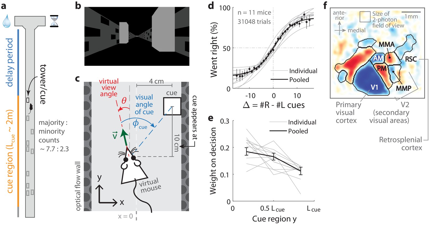
Two-photon calcium imaging of posterior cortical areas during a navigation-based evidence accumulation task.

(a) Layout of the virtual T-maze in an example left-rewarded trial. (b) Example snapshot of the cue region corridor from a mouse’s point of view when facing straight down the maze. Two cues on the right and left sides can be seen, closer and further from the mouse in that order. (c) Illustration of the virtual viewing angle θ. The visual angle $ϕ_{c u e}$ of a given cue is measured relative to θ and to the center of the cue. The y spatial coordinate points straight down the stem of the maze, and the $x$ coordinate is transverse. $\vec{v}$ is the velocity of the mouse in the virtual world. (d) Sigmoid curve fits to behavioral data for how frequently mice turned right for a given difference in total right vs. total left cue counts at the end of the trial, $Δ \equiv # R - # L$ . Dots: Percent of trials (out of those with a given $Δ$ ) in which mice turned right, pooling data from all mice. Error bars: 95% binomial C.I. (e) Logistic regression weights for predicting the mice’s choice given spatially-binned evidence ${Δ_{i}}$ where $i \in {1, 2, 3}$ indexes three equally sized spatial bins of the cue region. Error bars: 95% C.I. across bootstrap experiments. (f) Average visual field sign map ( $n = 5$ mice) and visual area boundaries, with all recorded areas labeled. The visual field sign is −1 (dark blue) where the cortical layout is a mirror image and +1 (dark red) where it follows a non-inverted layout of the physical world.

Figure 1—source data 1 Data points, summary statistics, and kernel bandwidths.: https://cdn.elifesciences.org/articles/60628/elife-60628-fig1-data1-v2.zip
Download elife-60628-fig1-data1-v2.zip

Figure 1—figure supplement 1

Download asset Open asset

Session-specific behavioral parameters, by mouse.

(a) Distribution (kernel density estimate) of session-average running speeds, for individual mice (columns). For each mouse, running speeds are sampled at the onset times of all the cues encountered in a given session, and then averaged across cue onsets for that session as a single entry in the distribution. (b) Distribution of session-specific standard deviation of running speeds, for individual mice (columns). Running speeds are computed as in (a), and then the standard deviation (instead of the mean) taken per session as a single entry in the mouse-specific distribution. (c) Session-average duration for which individual cues were visible to a given mouse (columns). The maximum duration is 200 ms after which cues were made to disappear, but shorter effective durations are possible if the mouse runs very quickly past the cue, causing it to move past the visual range of the VR display. Bars: 68% C.I. Lines: 95% C.I. (d) Session-specific standard deviation of cue visibility durations as in (c). Bars: 68% C.I. Lines: 95% C.I.

Figure 2 with 1 supplement

Download asset Open asset

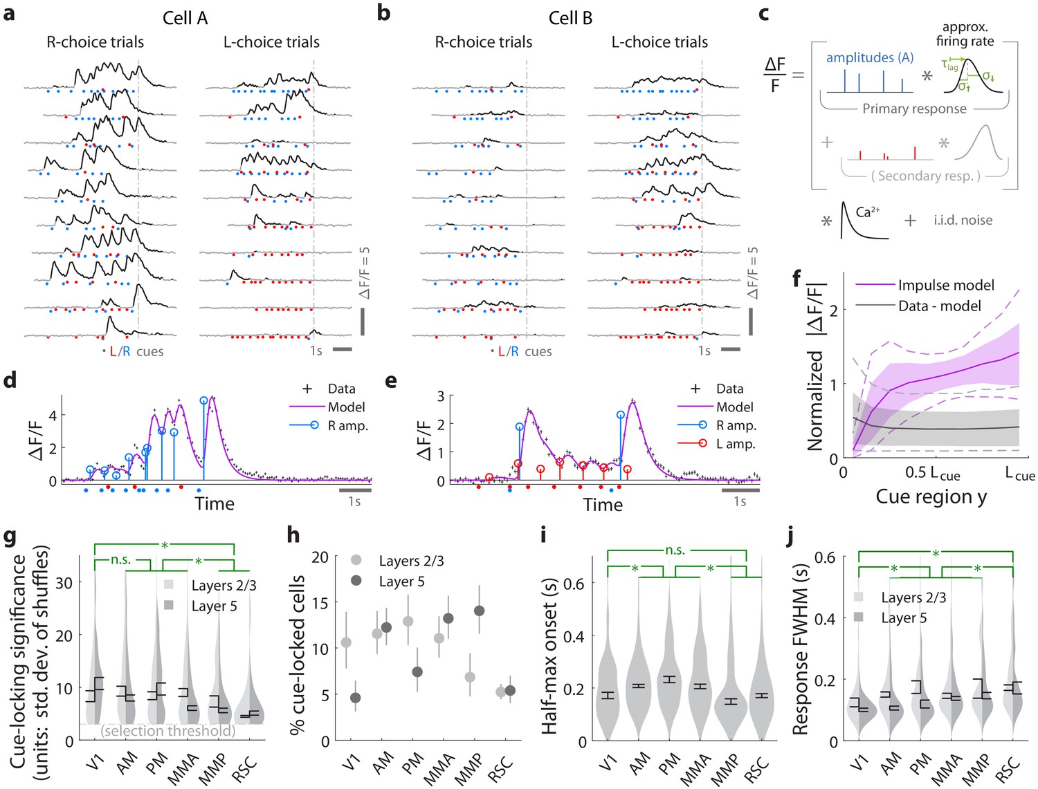
Pulses of evidence evoke transient, time-locked responses that are well described by an impulse response model.

(a) Trial-by-trial activity (rows) vs. time of an example right-cue-locked cell recorded in area AM, aligned in time to the end of the cue period (dashed line). Onset times of left (right) cues in each trial are shown as red (blue) dots. (b) Same as (a), but for an atypical right-cue-locked cell (in area AM) that has some left-cue-locked responses. (c) Depiction of the impulse response model for the activity level $Δ F / F$ of a neuron vs. time (x-axis). Star indicates the convolution operator. (d) Prediction of the impulse response model for the cell in (a) in one example trial. This cell had no significant secondary (left-cue) responses. (e) Same as (d) but for the cell in (b). The model prediction is the sum of primary (right-cue) and secondary (left-cue) responses. (f) Trial-average impulse response model prediction (purple) vs. the residual of the fit ( $Δ F / F$ data minus model prediction, black), in 10 equally sized spatial bins of the cue region. For a given cell, the average model prediction (or average residual) is computed in each spatial bin, then the absolute value of this quantity is averaged across trials, separately per spatial bin. Line: Mean across cells. Dashed line: 95% C.I. across cells. Band: 68% C.I. across cells. For comparability across cells, $Δ F / F$ was expressed in units such that the mean model prediction of each cell is 1. The model prediction rises gradually from baseline at the beginning of the cue period due to nonzero lags in response onsets. (g) Distribution (kernel density estimate) of cue-locking significance for cells in various areas/layers. Significance is defined per cell, as the number of standard deviations beyond the median AIC_C score of models constructed using shuffled data (Materials and methods). Error bars: S.E.M. of cells. Stars: significant differences in means (Wilcoxon rank-sum test). (h) Percent of significantly cue-locked cells in various areas/layers. Chance: $10^{- 3} %$ . Error bars: 95% binomial C.I. across sessions. (i) Distribution (kernel density estimate) of the half-maximum onset time of the primary response, for cells in various areas. Data were pooled across layers (inter-layer differences not significant). Error bars: S.E.M. across cells. Stars: significant differences in means (Wilcoxon rank-sum test). (j) As in (i) but for the full-width-at-half-max. Statistical tests use data pooled across layers. Means were significantly different across layers for areas AM and PM (Wilcoxon rank-sum test).

Figure 2—source data 1 Data points including individual entries for histograms, summary statistics and kernel bandwidths.: https://cdn.elifesciences.org/articles/60628/elife-60628-fig2-data1-v2.zip
Download elife-60628-fig2-data1-v2.zip

Figure 2—figure supplement 1

Download asset Open asset

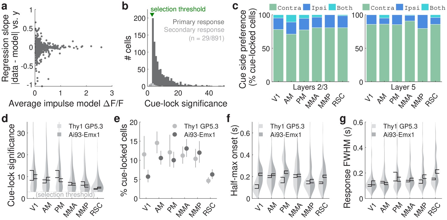
Additional statistics for cue-locked responses.

(a) Slope ( $β_{1}$ ) from a linear regression model $ρ = β_{0} + β_{1} y$ , where $ρ$ is the residual magnitude (absolute value of data minus impulse response model prediction) shown in Figure 2f, and $y$ is the spatial bin of the cue region in which the residual was computed (as explained for Figure 2f). Each point corresponds to a single significantly cue-locked cell. Residuals were normalized per cell by the average impulse model prediction (across trials and place in the cue region) for that cell; this normalization factor is also shown as the x-coordinate in the plot. Units were defined for the spatial bins such that 0 (1) corresponds to the start (end) of the cue region. A slope of ±1 can therefore be interpreted as a change in residuals from the start to the end of the cue region by an amount comparable to the mean signal predicted by the impulse response model. (b) Distribution of cue-locking significance for cells with a significant primary response (above five standard deviations compared to cues-shuffled fits). (c) Proportion of cells in various areas/layers that respond only to contralateral cues (green), only ipsilateral cues (dark blue), or to cues on both sides (light blue). (d–g) As in Figure 2g–j, but comparing data from two strains of mice. Data were pooled across layers.

Figure 3 with 3 supplements

Download asset Open asset

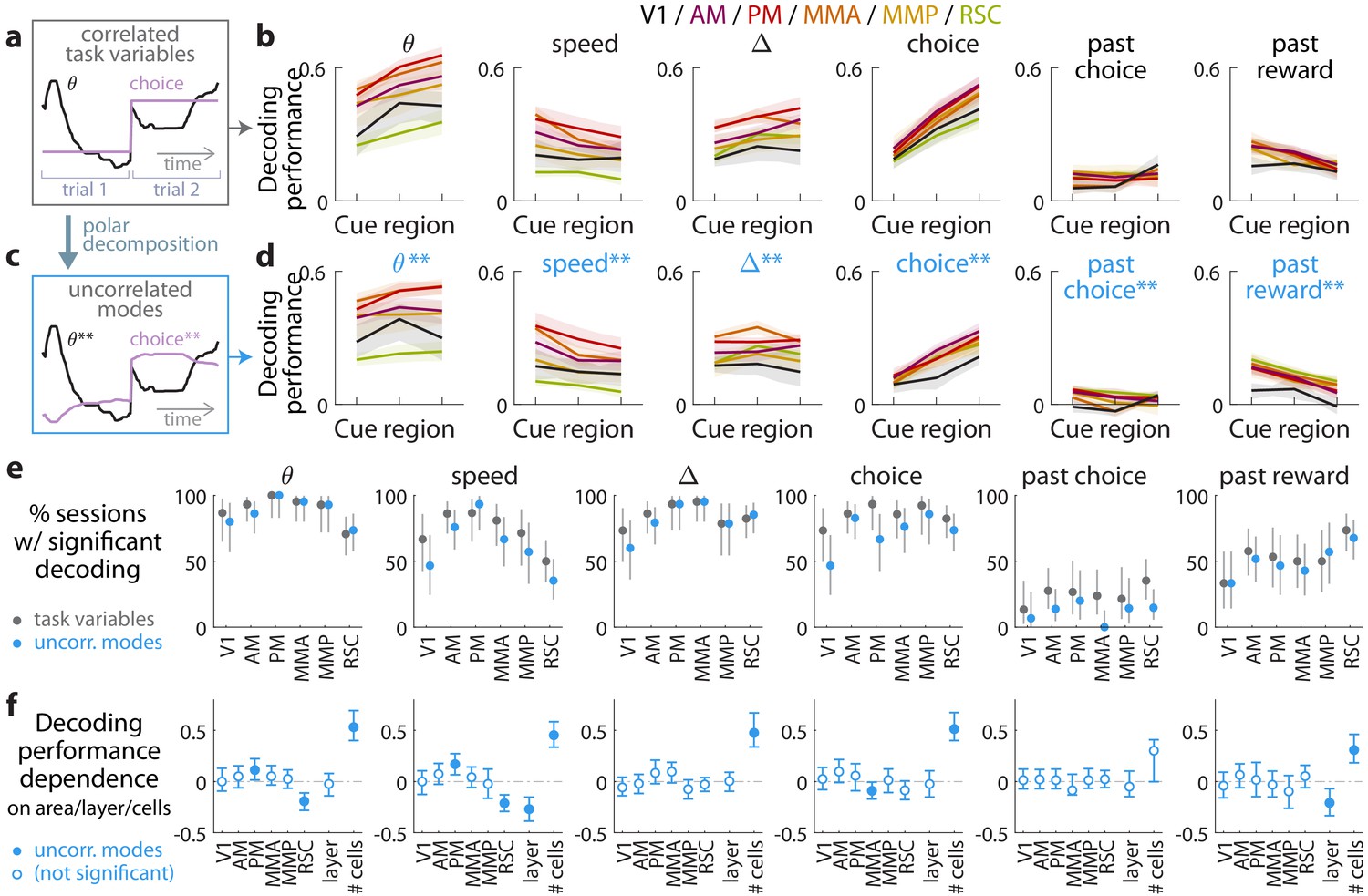
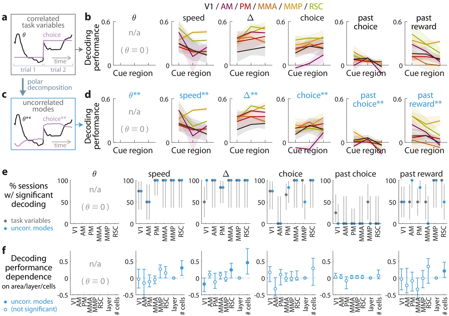
Multiple visual, motor, cognitive, and memory-related variables can be decoded from the amplitudes of cue-locked cell responses.

(a) Example time-traces of two statistically correlated task variables, the view angle $θ$ (black) and the eventual navigational choice (magenta). (b) Cross-validated performance for decoding six task variables (individual plots) from the amplitudes of cue-locked neuronal responses, separately evaluated using responses to cues in three spatial bins of the cue region (Materials and methods). The performance measure is Pearson’s correlation between the actual task variable value and the prediction using cue-locked cell amplitudes. Lines: mean performance across recording sessions for various areas (colors). Bands: S.E.M. across sessions, for each area. (c) Example time-traces of the two uncorrelated modes obtained from a polar decomposition of the correlated task variables in (a). This decomposition (Materials and methods) solves for these uncorrelated modes such that they were linear combinations of the original time-traces that were closest, in the least-squares sense, to the original traces, while constrained to be themselves uncorrelated with each other. Correlation coefficients between individual uncorrelated modes and their corresponding original variables were > 0.85 for all modes (Figure 3—figure supplement 1). (d) As in (a), but for decoding the uncorrelated task-variable modes illustrated in (c). (e) Proportion of imaging sessions that had significant decoding performance for the six task variables in (b) (dark gray points) and uncorrelated modes in (d) (blue points), compared to shuffled data and corrected for multiple comparisons. Data were restricted to 140/143 sessions with at least one cue-locked cell. Error bars: 95% binomial C.I. across sessions. (f) Linear regression (Support Vector Machine) weights for how much the decoding performance for uncorrelated task-variable modes in (d) depended on cortical area/layer and number of recorded cue-locked cells. The decoder accuracy was evaluated at the middle of the cue region for each dataset. The area and layer regressors are indicator variables, e.g. a recording from layer 5 of V1 would have regressor values (V1 = 1, AM = 0, PM = 0, MMA = 0, MMP = 0, RSC = 0, layer = 1). Weights that are not statistically different from zero are indicated with open circles. The negative weight for layer dependence of past-reward decoding means that layer five had significantly lower decoding performance than layers 2/3. Error bars: 95% C.I. computed via bootstrapping sessions.

Figure 3—source data 1 Data points and summary statistics.: https://cdn.elifesciences.org/articles/60628/elife-60628-fig3-data1-v2.zip
Download elife-60628-fig3-data1-v2.zip

Figure 3—figure supplement 1

Download asset Open asset

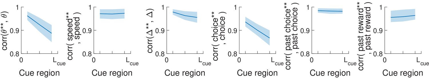
Pearson’s correlation between uncorrelated behavioral modes (θ**, speed**, etc.) and the corresponding most similar task variable (θ, speed, etc.).

These uncorrelated modes were computed via polar decomposition as explained in the Materials and methods. Bands: standard deviation across imaging sessions.

Figure 3—figure supplement 2

Download asset Open asset

Qualitatively similar performances for decoding task variables from cue-locked response amplitudes in control experiments with view-angle restricted to zero in the cue region.

(a–f) As in Figure 3, but using data from the θ-controlled experiments.

Figure 3—figure supplement 3

Download asset Open asset

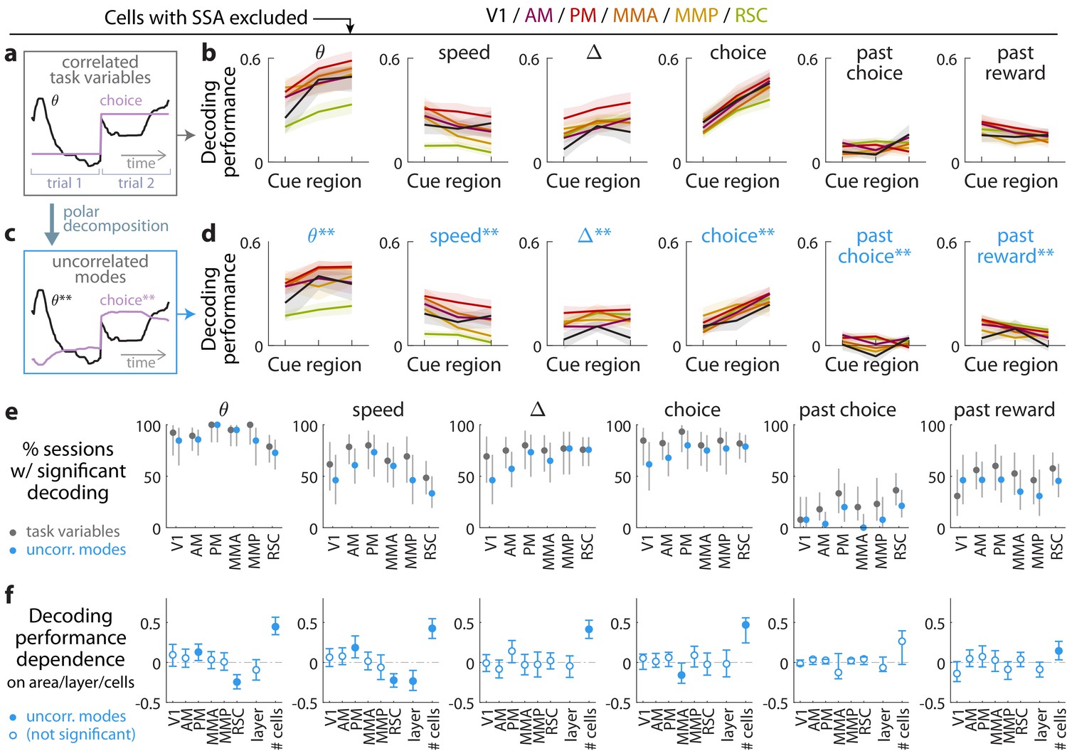
Evidence (and other task variables) can still be decoded from cue-locked response amplitudes, excluding cells that exhibit stimulus-specific adaptation (SSA).

(a–f) As in Figure 3, but with cells that favored the SSA model excluded from the data.

Figure 4 with 2 supplements

Download asset Open asset

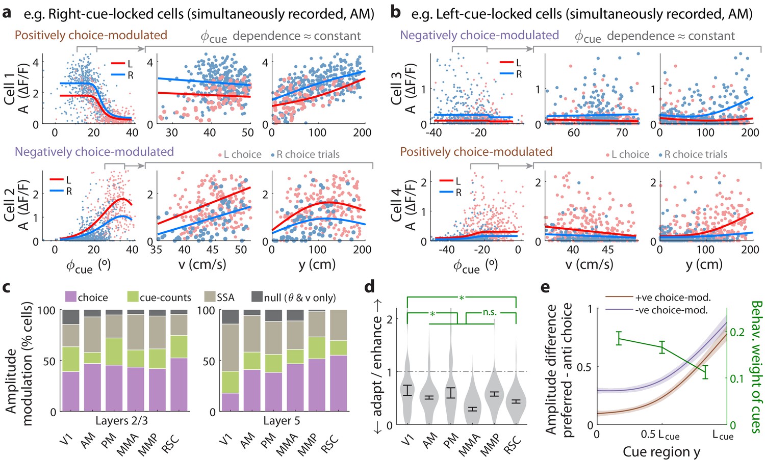
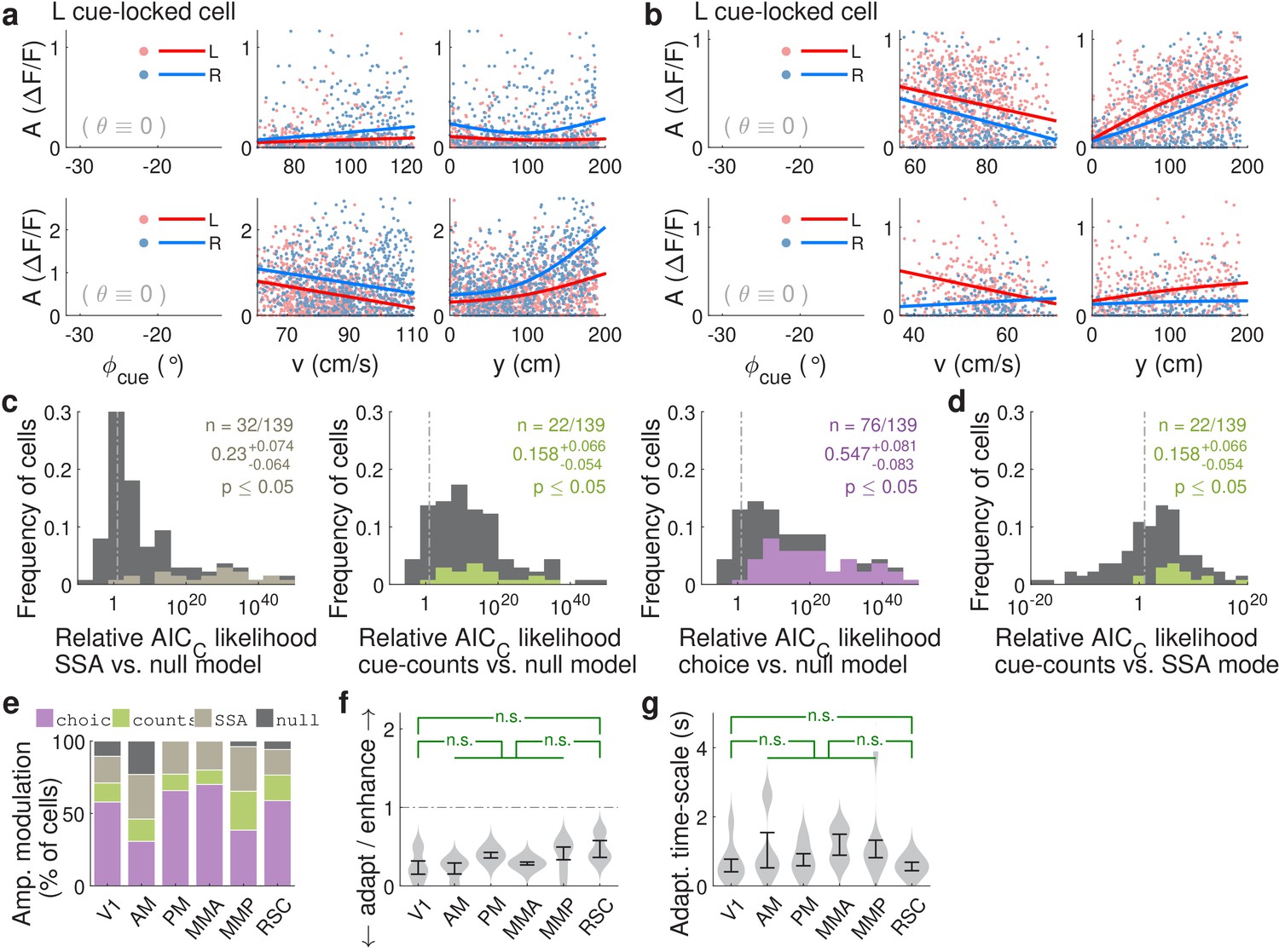
Cue-locked response amplitudes depend on view angle, speed, and cue frequency, but a large fraction exhibit choice-related modulations that increase during the course of the trial.

(a) Response amplitudes of two example right-cue-locked cells (one cell per row) vs. (columns) the visual angle at which the cue appeared ( $ϕ_{c u e}$ ), running speed ( $v$ ), and $y$ location of the cue in the cue region. Points: amplitude data in blue (red) according to the upcoming right (left) choice. Lines: AIC_C-weighted model mean functions for right- vs. left-choice trials (lines); the model predicts the data to be random samples from a Gamma distribution with this behavior-dependent mean function. The data in the right two columns were restricted to a subset where angular receptive field effects are small, corresponding to the indicated area in the leftmost plots. (b) Same as (a) but for two (left-cue-locked) cells with broader angular receptive fields. (c) Percentages of cells that significantly favor various amplitude modulation models (likelihood ratio <0.05, defaulting to null model if none are significant), in the indicated cortical areas and layers. For layer 2/3 data, V1 has a significantly higher fraction of cells preferring the null model than other areas (p = 0.02, two-tailed Wilcoxon rank-sum test). For layer 5 data, V1 has a significantly lower choice-model preferring fraction than the other areas (p = 0.003). (d) Distribution (kernel density estimate) of adaptation/enhancement factors for cells that favor the SSA model. A factor of 1 corresponds to no adaptation, while for other values the subsequent response is scaled by this amount with exponential recovery toward 1. Error bars: S.E.M. Stars: significant differences in means (Wilcoxon rank-sum test). (e) Comparison of the behaviorally deduced weighting of cues (green, same as Figure 1e) to the neural choice modulation strength vs. location in the cue region (for contralateral-cue-locked cells only, but ipsilateral-cue-locked cells in Figure 4—figure supplement 2g have similar trends). The choice modulation strength is defined using the amplitude-modulation model predictions, and is the difference between predicted amplitudes on preferred-choice minus anti-preferred-choice trials, where preferred choice means that the neuron will have higher amplitudes on trials of that choice compared to trials of the opposite (anti-preferred) choice. For comparability across cells, the choice modulation strength is normalized to the average amplitude for each cell (Materials and methods). Lines: mean across cue-locked cells, computed separately for positively vs. negatively choice-modulated cells (data from all brain regions). Bands: S.E.M.

Figure 4—source data 1 Data points and summary statistics.: https://cdn.elifesciences.org/articles/60628/elife-60628-fig4-data1-v2.zip
Download elife-60628-fig4-data1-v2.zip

Figure 4—figure supplement 1

Download asset Open asset

Qualitatively similar cue-locked amplitude modulations in control experiments with view angle restricted to be zero in the cue region.

(a–b,e–f) As in Figure 4, except using data from the control experiments. (c–d,g) As in Figure 4—figure supplement 2a–b,d, except using data from the θ-controlled experiments.

Figure 4—figure supplement 2

Download asset Open asset

Additional statistics for amplitude modulations of cue-locked cells.

(a) Distribution of AIC_C likelihood ratios for various amplitude-modulation models vs. the null hypothesis where cell responses only depend on an angular receptive field and speed. Colored areas corresponds to cells for which the indicated model is the best model for that cell (likelihood ratio n < 0.05). Data were pooled across all sessions. Note the logarithmic x-axis scale. (b) As in (a), distribution of AIC_C likelihood ratios for cue-counts model vs. the SSA model. Colored areas corresponds to cells for which the cue-counts model was the best model for that cell (likelihood ratio <0.05). (c) Distribution (kernel density estimate) of predicted speed-induced changes in amplitudes for a change in speed of 10 cm/s. Data were pooled across layers. Error bars: S.E.M. across cells. Stars: significant differences in means (Wilcoxon rank-sum test). (d) Distribution of adaptation/enhancement timescales for cells that favor the SSA model, defined as the time taken for the amplitude to recover to baseline by a factor of $1 / e$ . Error bars: S.E.M. across cells. Stars: significant differences in means (Wilcoxon rank-sum test). (e) Distribution of choice modulation effect sizes for cue-locked cells in various areas/layers, defined as the maximum difference in predicted responses on contralateral- vs. ipsilateral-choice trials, divided by the mean response. Cells with numerically near-zero modulations ( $| δ A^{c h o i c e} | \leq 10^{- 4}$ ) were excluded. Error bars: S.E.M. across cells. (f) Proportions out of all significantly cue-counts-modulated cells for which the best model is that which depends on the difference (left columns) in or single-side counts (middle and right columns) of cues, and shown separately for contralateral- and ipsilateral-cue-locked cells. Error bars: 95% C.I. across cells. (g) As in Figure 4e, but for ipsilateral-cue-locked cells. (h) As in Figure 4c, but for mice of two different strains. Data were pooled across layers.

Figure 4—figure supplement 2—source data 1 Summary statistics.: https://cdn.elifesciences.org/articles/60628/elife-60628-fig4-figsupp2-data1-v2.zip
Download elife-60628-fig4-figsupp2-data1-v2.zip

Figure 5

Download asset Open asset

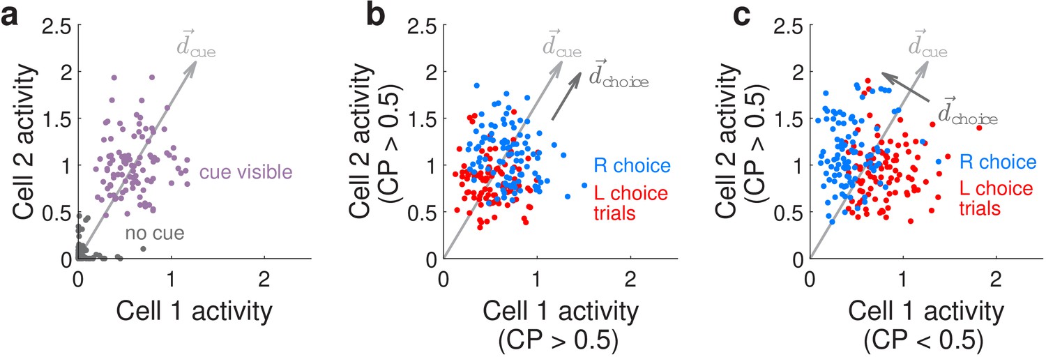
Conceptualization of how choice-related modulations can modify sensory representations at the neural-population level.

(a) Illustrated distribution of the joint activity levels (‘neural state’) of two cue-locked cells, at time-points when there is no visual cue (dark gray), vs. time-points when a cue of the preferred laterality for these cells (purple) is present. Each time-point in this simulation corresponds to different samples of noise in the two neural responses, which results in variations in the neural state (multiple dots each corresponding to a different neural state). ${\vec{d}}_{c u e}$ is a direction that best separates neural states for the ‘no cue’ vs. ‘cue visible’ conditions. (b) Illustrated distribution of neural states as in (a), but for time-points when a cue is present, colored differently depending on whether the mouse will eventually make a right-turn (blue) or left-turn choice. ${\vec{d}}_{c h o i c e}$ is a direction that best separates neural states for right- vs. left-choice conditions, which was chosen here to be parallel to ${\vec{d}}_{c u e}$ (defined as in (a)). (c) Same as (b), but for a scenario where ${\vec{d}}_{c h o i c e}$ was chosen to be orthogonal to ${\vec{d}}_{c u e}$ .

Additional files

Supplementary file 1 Number of imaging sessions and mice for various areas and layers, for the main experiment.: https://cdn.elifesciences.org/articles/60628/elife-60628-supp1-v2.docx
Download elife-60628-supp1-v2.docx
Supplementary file 2 Overall performance and number of imaging sessions for the main experiment, per mouse (rows), in various areas and layers (columns). Mice of the Thy1 GP5.3 strain have names starting with ‘gp’, and those from the Ai93-Emx1 strain have names starting with ‘ai’ (see Materials and methods).: https://cdn.elifesciences.org/articles/60628/elife-60628-supp2-v2.docx
Download elife-60628-supp2-v2.docx
Transparent reporting form: https://cdn.elifesciences.org/articles/60628/elife-60628-transrepform-v2.docx
Download elife-60628-transrepform-v2.docx

Download links

A two-part list of links to download the article, or parts of the article, in various formats.

Downloads (link to download the article as PDF)

Open citations (links to open the citations from this article in various online reference manager services)

Mendeley

Cite this article (links to download the citations from this article in formats compatible with various reference manager tools)

Sue Ann Koay
Stephan Thiberge
Carlos D Brody
David W Tank

(2020)

Amplitude modulations of cortical sensory responses in pulsatile evidence accumulation

eLife 9:e60628.

https://doi.org/10.7554/eLife.60628

Sign up for email alerts

Privacy notice