Freshwater monitoring by nanopore sequencing
- European Bioinformatics Institute, Wellcome Genome Campus, United Kingdom
- Department of Plant Sciences, University of Cambridge, United Kingdom
- Department of Earth Sciences, University of Cambridge, United Kingdom
- Department of Engineering, University of Cambridge, United Kingdom
- Department of Biochemistry, University of Cambridge, United Kingdom
- Wellcome Sanger Institute, Wellcome Trust Genome Campus, United Kingdom
- Department of Physics, University of Cambridge, United Kingdom
- Department of Physiology, Development & Neuroscience, University of Cambridge, United Kingdom
- Department of Veterinary Medicine, University of Cambridge, United Kingdom
Figures
Figure 1 with 1 supplement
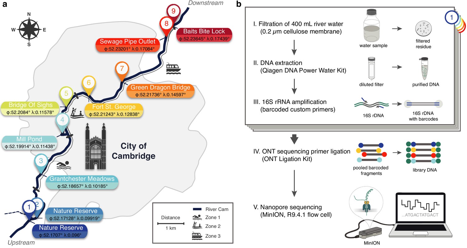
Freshwater microbiome study design and experimental setup.
(a) Schematic map of Cambridge (UK), illustrating sampling locations (colour-coded) along the River Cam. Geographic coordinates of latitude and longitude are expressed as decimal fractions according to the global positioning system. (b) Laboratory workflow to monitor bacterial communities from freshwater samples using nanopore sequencing (Materials and methods).
Figure 1—figure supplement 1

Bioinformatics consensus workflow.
Essential data processing steps, from nanopore sequencing to spatiotemporal bacterial composition analysis (Materials and methods). After full-length 16S rDNA sequencing with the MinION (R9.4.1 flow cell), local basecalling of the raw fast5 files was performed using Guppy (Wick et al., 2019). Output fastq files were filtered for length and quality (Materials and methods), and reads assigned to their location barcode using Porechop. We then used Minimap2 (k = 15) and the SILVA v.132 database for taxonomic classifications. Rarefaction reduced each sample to the same number of reads (37,000), allowing for a robust comparison of bacterial composition across samples in various analyses.
Figure 2 with 2 supplements
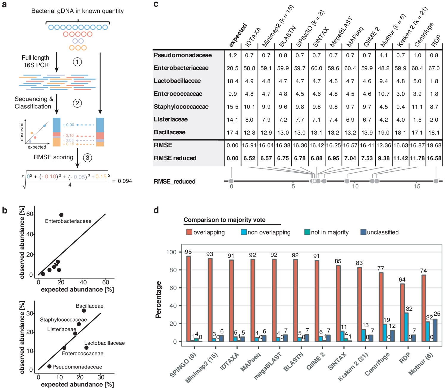
Benchmarking of classification tools with nanopore full-length 16S sequences.
(a) Schematic of mock community quantification performance testing. (b) Observed vs. expected read fraction of bacterial families present in 10,000 nanopore reads randomly drawn from mock community sequencing data. Example representation of Minimap2 (kmer length 15) quantifications with (upper) and without (lower) Enterobacteriaceae (Materials and methods). (c) Mock community classification output summary for twelve classification tools tested against the same 10,000 reads. Root mean squared errors observed and expected bacterial read fractions are provided with (RMSE) and without Enterobacteriaceae (RMSE reduced). (d) Classification output summary for 10,000 reads randomly drawn from an example freshwater sample (Materials and methods). ‘Overlapping’ fractions (red) represent agreements of a classification tool with the majority of tested methods on the same reads, while ‘non-overlapping’ fractions (light blue) represent disagreements. Dark green sets highlight rare taxon assignments not featured in any of the 10,000 majority classifications, while dark blue bars show unclassified read fractions.
Figure 2—figure supplement 1
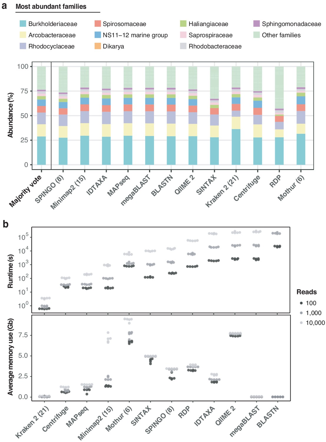
Benchmarking of twelve taxonomic classifiers with nanopore full-length 16S sequences.
(a) Top 10 represented bacterial taxon families across all methods, based on the 10,000 aquatic reads used in Figure 2d. (b) Comparison of computational performances with respect to (upper) runtime and average memory (lower) usage for the classification of 5 × 100, 5 × 1000, and 5 × 10,000 random read draws of the same sample. BLASTN-based classifications of 10,000 read sets are omitted, as their runtimes exceeded 14 days (> 106 s). Numbers in brackets for SPINGO, Minimap2, Kraken 2 and Mothur indicate kmer sizes.
Figure 2—figure supplement 2
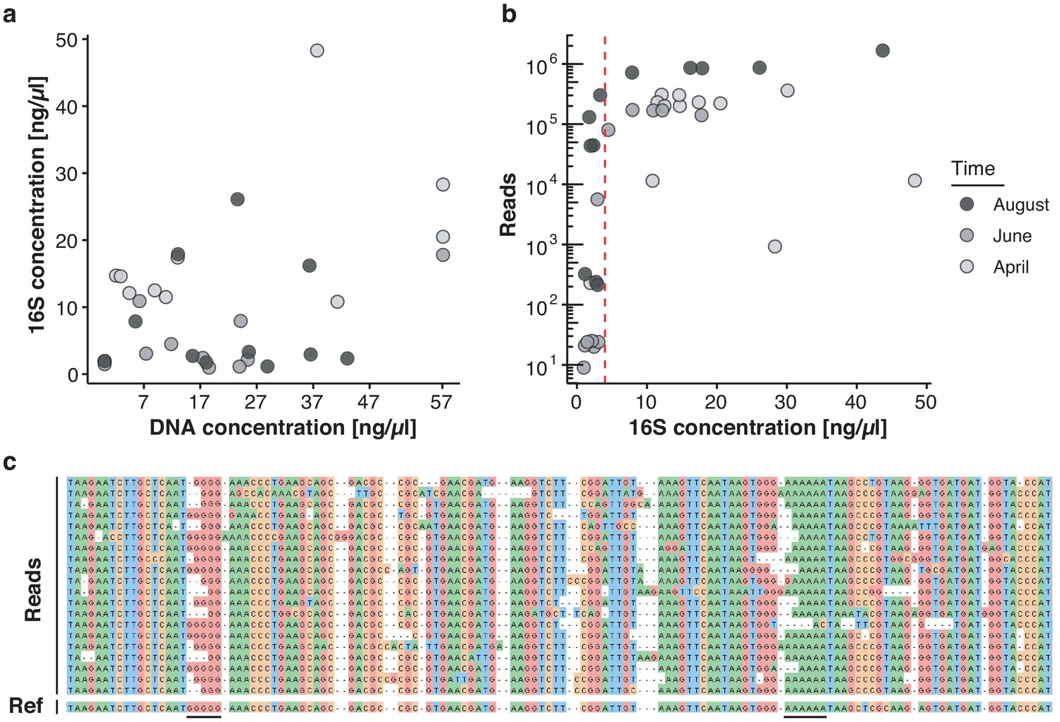
Key challenges of freshwater monitoring with nanopore sequencing.
(a–b) Correlation analysis between DNA extraction yield, 16S amplification yield and raw sequencing output (Supplementary file 2). (a) DNA concentrations (x-axis) obtained from 30 freshwater samples after extraction with the DNeasy PowerWater Kit (Materials and methods) are compared against the DNA concentration of the same samples after full-length 16S PCR amplification (y-axis), as measured by Qubit dsDNA HS. (b) The DNA concentration obtained for each sample after full-length 16S PCR amplification (x-axis) is compared against the final number of demultiplexed nanopore sequencing reads. Samples with a minimum input concentration measurement of ~5 ng/µl yielded sequencing outputs sufficient to pass the rarefaction threshold of 37,000 reads. (c) Multiple sequence alignment of an example set of related nanopore 16S sequences, displaying increased indel rates at homopolymer reference sites (underlined); the mean sequencing error rate for this study lies at 7.92%.
Figure 3 with 1 supplement
Bacterial diversity of the River Cam.
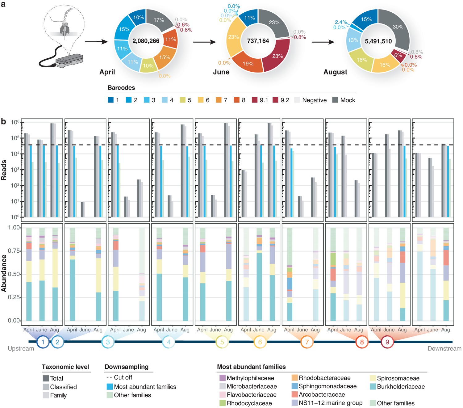
(a) Nanopore sequencing output summary. Values in the centre of the pie charts depict total numbers of classified nanopore sequences per time point. Percentages illustrate representational fractions of locations and control barcodes (negative control and mock community). (b) Read depth and bacterial classification summary. Upper bar plot shows the total number of reads, and the number of reads classified to any taxonomic level, to at least bacterial family level, to the ten most abundant bacterial families across all samples, or to other families. Rarefaction cut-off displayed at 37,000 reads (dashed line). Lower bar plot features fractions of the ten most abundant bacterial families across the samples with more than 100 reads. Colours in bars for samples with less than 37,000 reads are set to transparent.
Figure 3—figure supplement 1
Impact of rarefaction on diversity estimation.
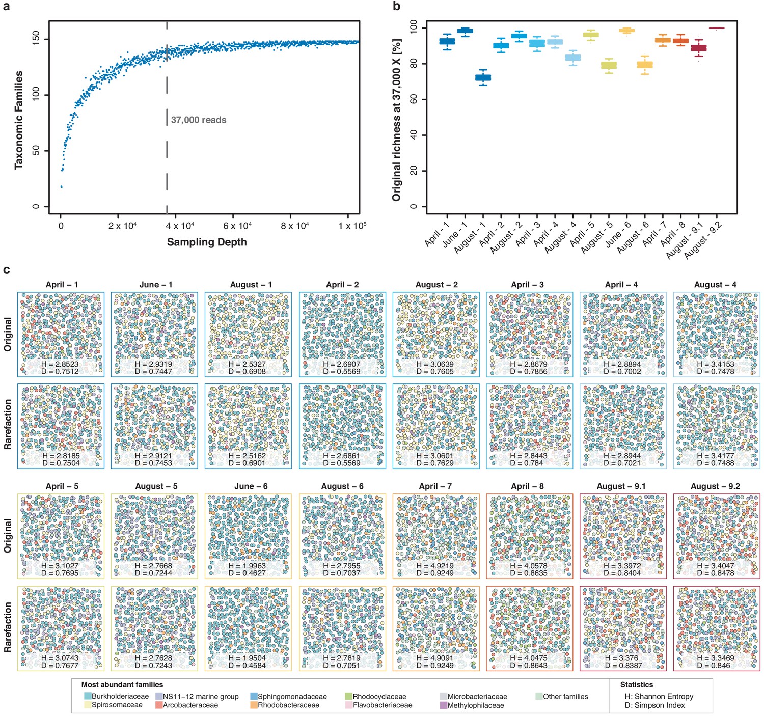
(a) Example rarefaction curve for bacterial family classifications of the 'April-1' sample. The chosen cut-off preserves most (~90%) of the original family taxon richness (vertical line). (b) Difference between original and rarefied family richness at 37,000 reads across all freshwater sequencing runs with quantitative sequencing outputs above the chosen cut-off. Boxplots feature 100 independent rarefactions per sample. Error bars represent Q1 – 1.5*IQR (lower), and Q3 + 1.5*IQR (upper), respectively. (c) Diversity visualisation of the ten most abundant bacterial families across all samples with sequencing outputs > 37,000 reads, through 400 ‘unordered bubbles’. Taxonomic proportions and colours are in accordance with Figure 3b. Shannon (H) and Simpson (D) indices for all samples indicate marginal differences between pairs of original and rarefied sets.
Figure 4 with 1 supplement
Core microbiome of the River Cam.
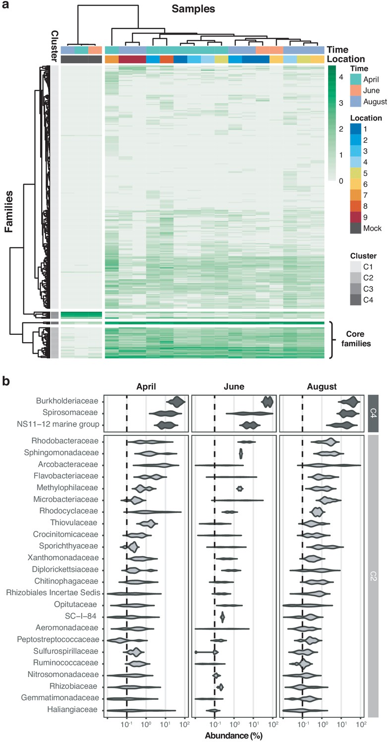
(a) Hierarchical clustering of bacterial family abundances across freshwater samples after rarefaction, together with the mock community control. Four major clusters of bacterial families occur, with two of these (C2 and C4) corresponding to the core microbiome of ubiquitously abundant families, one (C3) corresponding to the main mock community families and one (C1) corresponding to the majority of rare accessory taxa. (b) Detailed river core microbiome. Violin plots summarise fractional representation of bacterial families from clusters C2 and C4 (log10 scale of relative abundance [%] across all samples, nApril = 7, nJune = 2, nAugust = 7), sorted by median total abundance. Vertical dashed lines depict 0.1% proportion.
Figure 4—figure supplement 1
River Cam core microbiome analysis on the bacterial genus level.
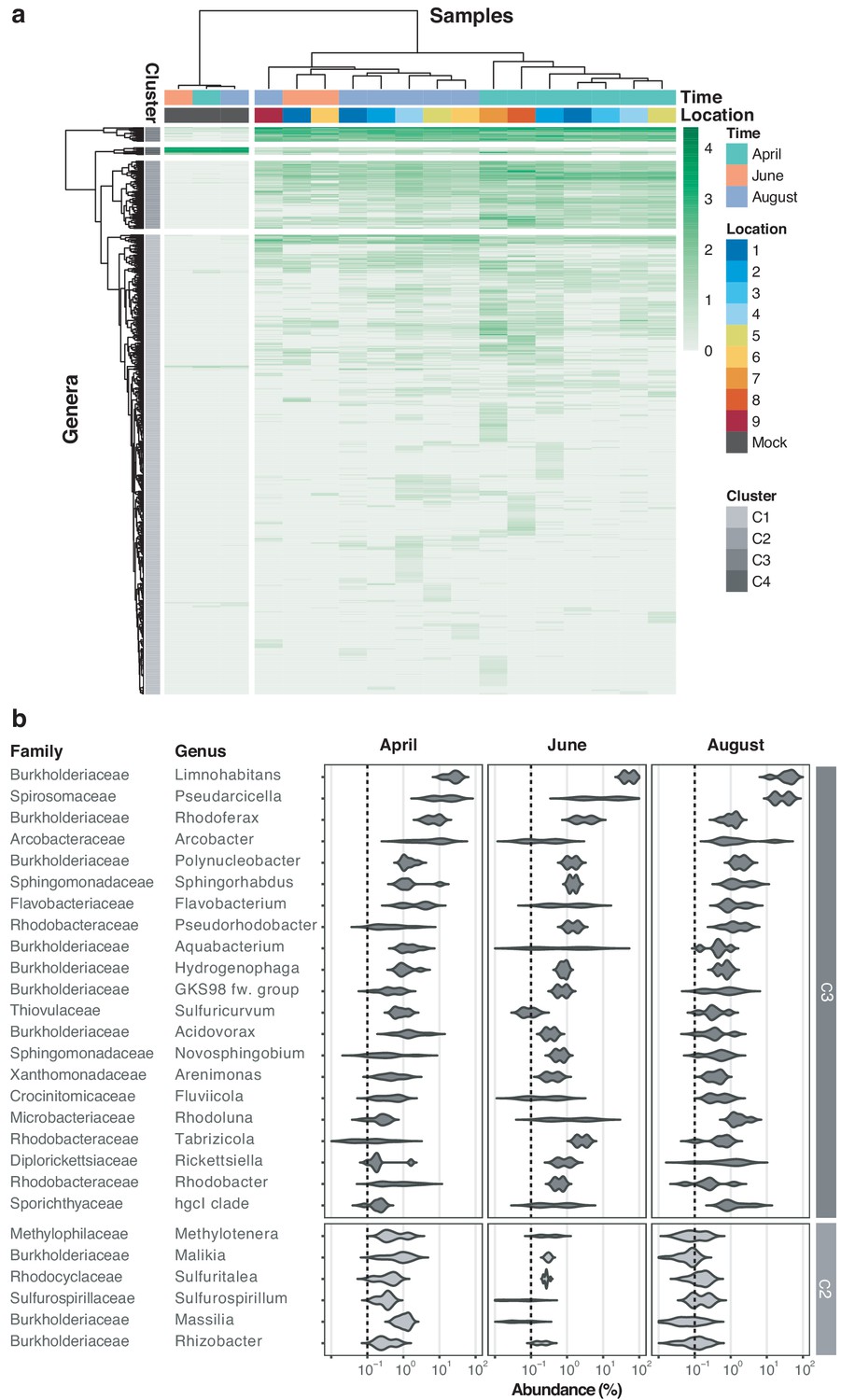
(a) Hierarchical clustering of bacterial genera abundances across freshwater samples after rarefaction, together with the mock community control. In similarity to the family analysis displayed in Figure 4, bacterial genera are clustered into four groups. Two of these (C3 and partially C2) correspond to the core microbiome of ubiquitously abundant genera, one (C4) corresponding to the main mock community genera and one (C1) corresponding to the majority of rare accessory taxa. (b) Dominant river core microbiome on the genus level. Violin plots (log10 scale of relative abundance [%] across all samples, nApril = 7, nJune = 2, nAugust = 6) summarise fractional representation of the top 27 bacterial genera and corresponding families from clusters C2 and C3, sorted by median total abundance. Vertical dashed line depicts 0.1% proportion. Out of the top 16 core families (Figure 4b), only the NS11-12 marine group family was found not to be represented on the genus level; NS11-12 marine group genera are mainly composed of uncultured bacteria, which here could not be classified at higher resolution.
Figure 5 with 1 supplement

Spatiotemporal axes of taxonomic diversity in the River Cam.
(a) PCA of bacterial composition across locations, indicating community dissimilarities along the main time (PC3) and spatial (PC4) axes of variation; dots coloured according to time points. Kruskal-Wallis test on PC3 component contributions, with post-hoc Mann-Whitney U rank test (April vs. August): p = 2.2*10−3. (b) Contribution of individual bacterial families to the PCs in (a). Error bars represent the standard deviation of these families across four independent rarefactions.
Figure 5—figure supplement 1
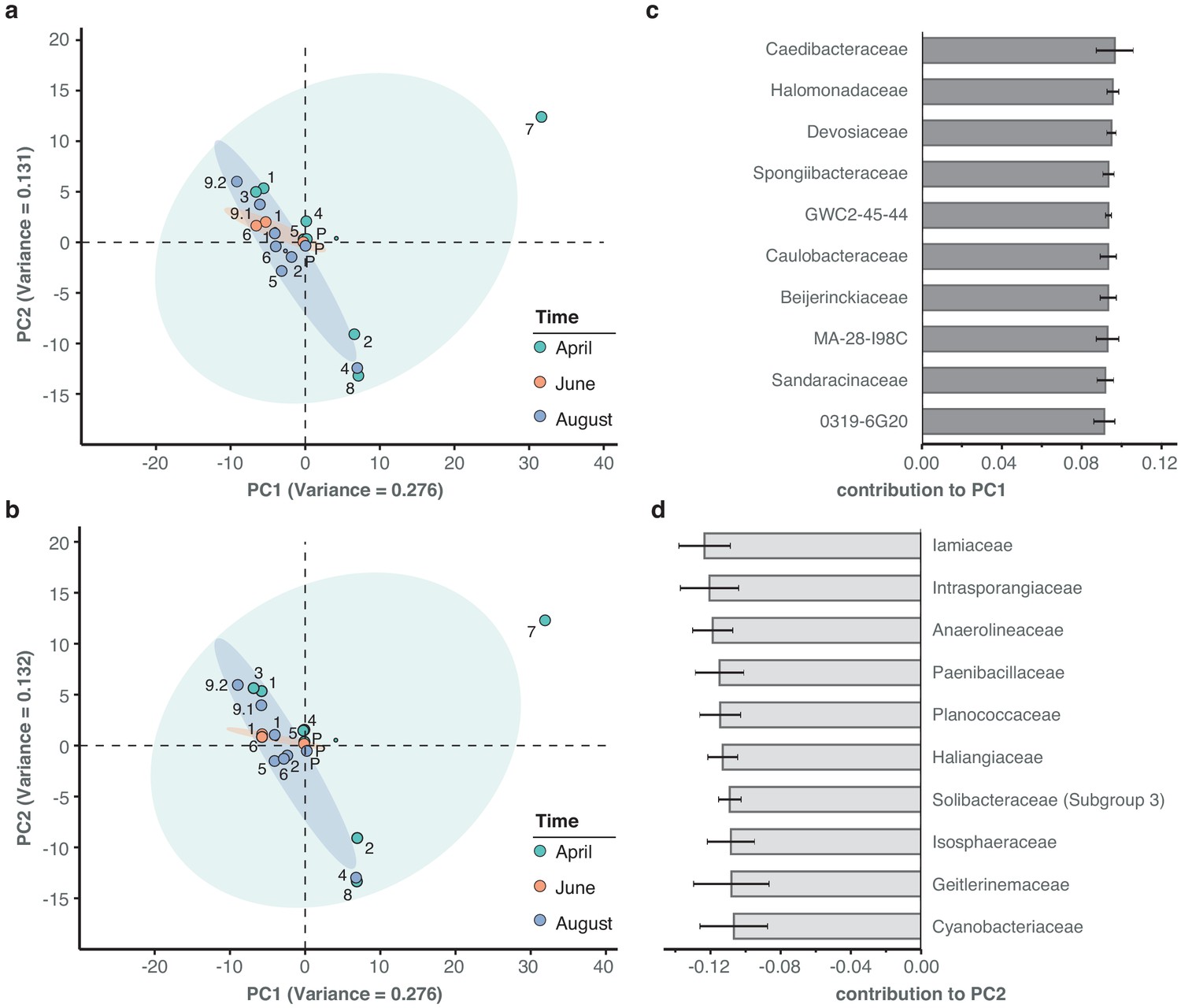
Principal component analysis of river bacterial family compositions.
(a–b) PCA with two independent rarefaction sets to 37,000 reads in all freshwater sequencing samples. Numbers and coloured dots indicate locations for each time point. The first and second principal components (PC1 and PC2, combined variance:~41%) robustly capture outlier samples 'April-7' along PC1 and 'April-2', 'August-4' and 'April-8' along PC2. (c–d) Fractional loads of the ten bacterial families most strongly contributing to changes along PC1 (c) and along PC2 (d). Error bars represent standard deviation of these families to the respective PC across four independent rarefactions. Subsequent principal components (PC3 and PC4) are less outlier-driven and depict spatial and temporal metagenomic trends within the River Cam.
Figure 6 with 1 supplement
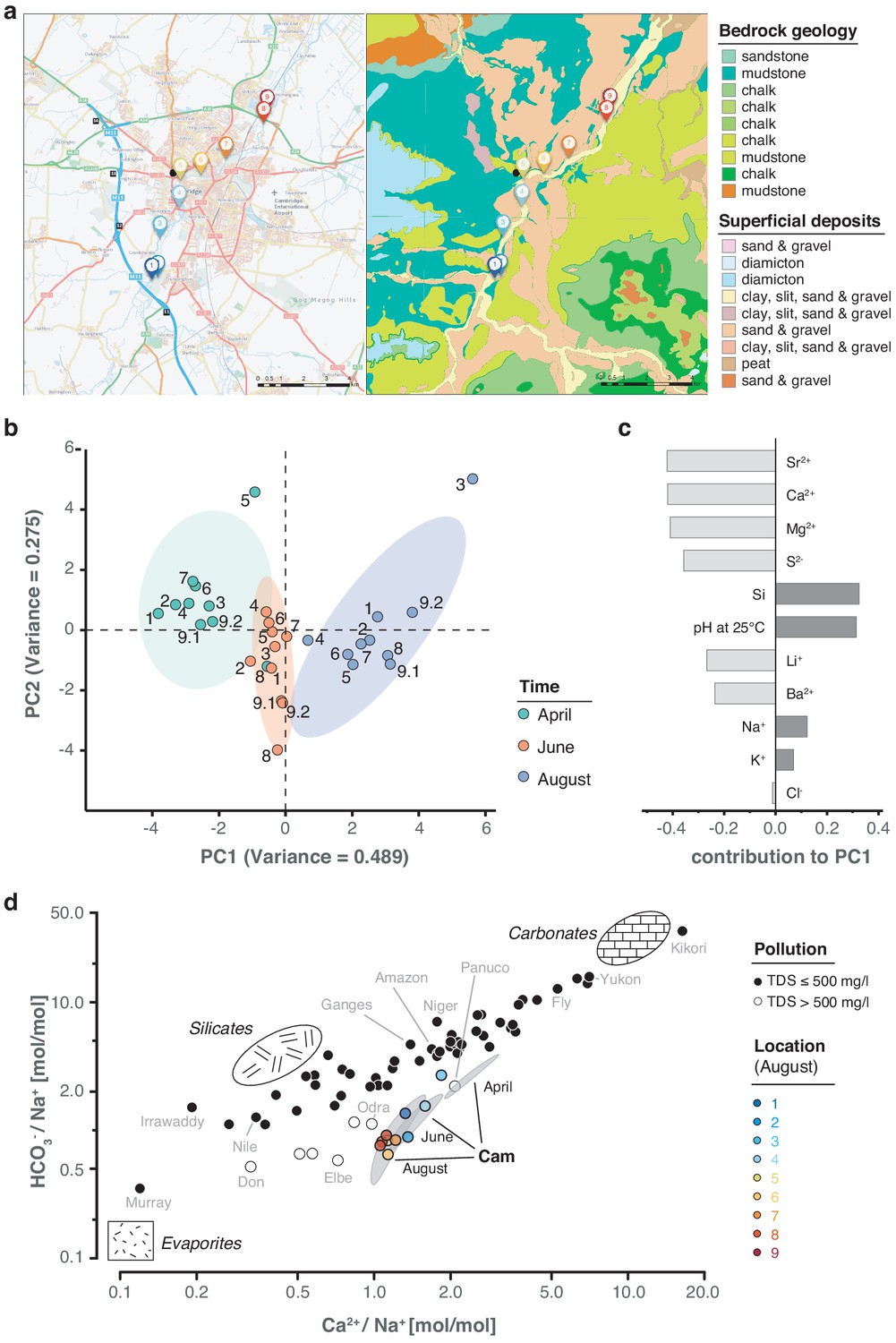
Geological and hydrochemical profile of the River Cam and its basin.
(a) Outline of the Cam River catchment surrounding Cambridge (UK), and its corresponding lithology. Overlay of bedrock geology and superficial deposits (British Geological Survey data: DiGMapGB-50, 1:50,000 scale) is shown as visualised by GeoIndex. Bedrock is mostly composed of subtypes of Cretaceous limestone (chalk), gault (clay, sand), and mudstone. Approximate sampling locations are colour-coded as in Figure 1. (b) Principal component analysis of measured pH and 13 inorganic solute concentrations of this study's 30 river surface water samples. PC1 (~49% variance) displays a strong, continuous temporal shift in hydrochemistry. (c) Parameter contributions to PC1 in (b), highlighting a reduction in water hardness (Ca2+, Mg2+) and increase in pH towards the summer months (June and August). (d) Mixing diagram with Na+-normalised molar ratios, representing inorganic chemistry loads of the world's 60 largest rivers; open circles represent polluted rivers with total dissolved solid (TDS) concentrations > 500 mg l−1. Cam River ratios are superimposed as ellipses from ten samples per month (50% confidence, respectively). Separate data points for all samples from August are also shown and colour-coded, indicating the upstream-to-downstream trend of Na+ increase (also observed in April and June). End-member signatures show typical chemistry of small rivers draining these lithologies exclusively (carbonate, silicate and evaporite).
Figure 6—figure supplement 1
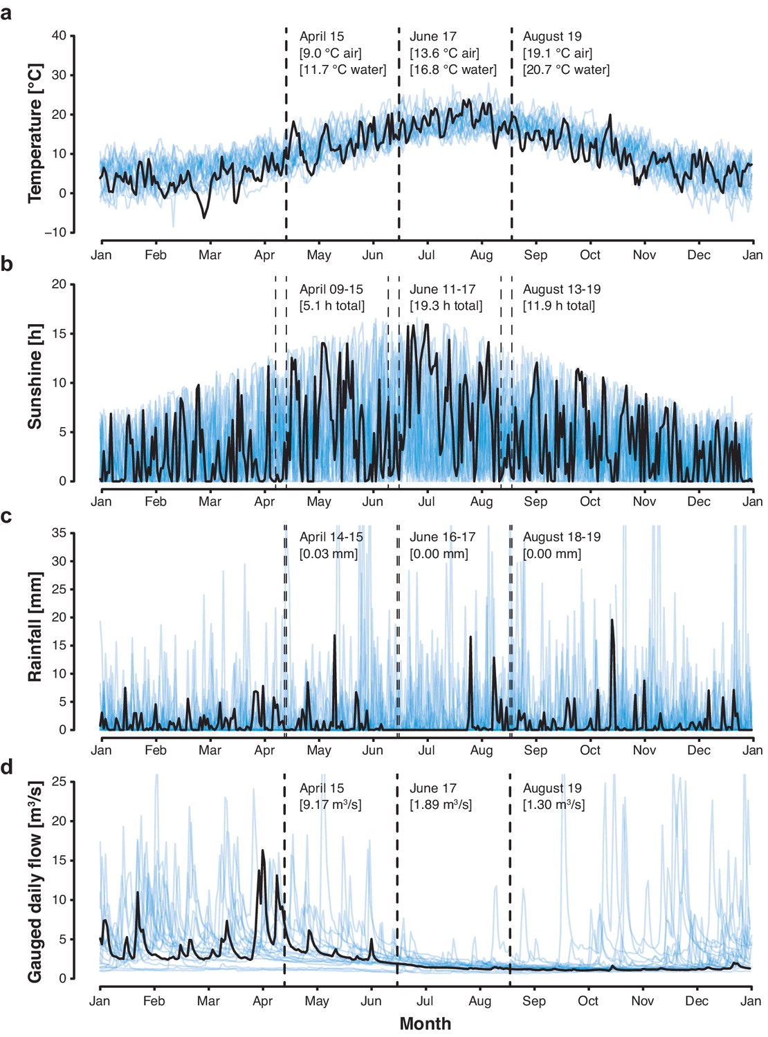
Cambridge weather and River Cam flow rate.
(a) Daily air temperature [°C], (b) daily sunshine [hr], and (c) daily rainfall [mm] of Cambridge in 2018 (black trend line) vs. 1998–2017 (blue background trend lines). (d) Cam River gauged daily flow [m3s−1] in 2018 (black trend line) vs. 1968–2017 (blue background trend lines). Data was compiled from public repositories https://www.cl.cam.ac.uk/research/dtg/weather/ and https://nrfa.ceh.ac.uk/. Gauged daily flow measurements at Jesus Lock, Cambridge (between sampling locations 5 and 6; NRFA #33016) were discontinued in 1983. Yet, contemporary flow rates can be modelled with high accuracy (Pearson's R = 0.9, R2 = 0.8) through linear data integration of three upstream stations already in operation since before 1983: Rhee at Wimpole (NRFA #33027, 70.2% model weight), Granta at Stapleford (NRFA #33053, 19.6% model weight) and Cam at Dernford (NRFA #33024, 10.3% model weight).
Figure 7
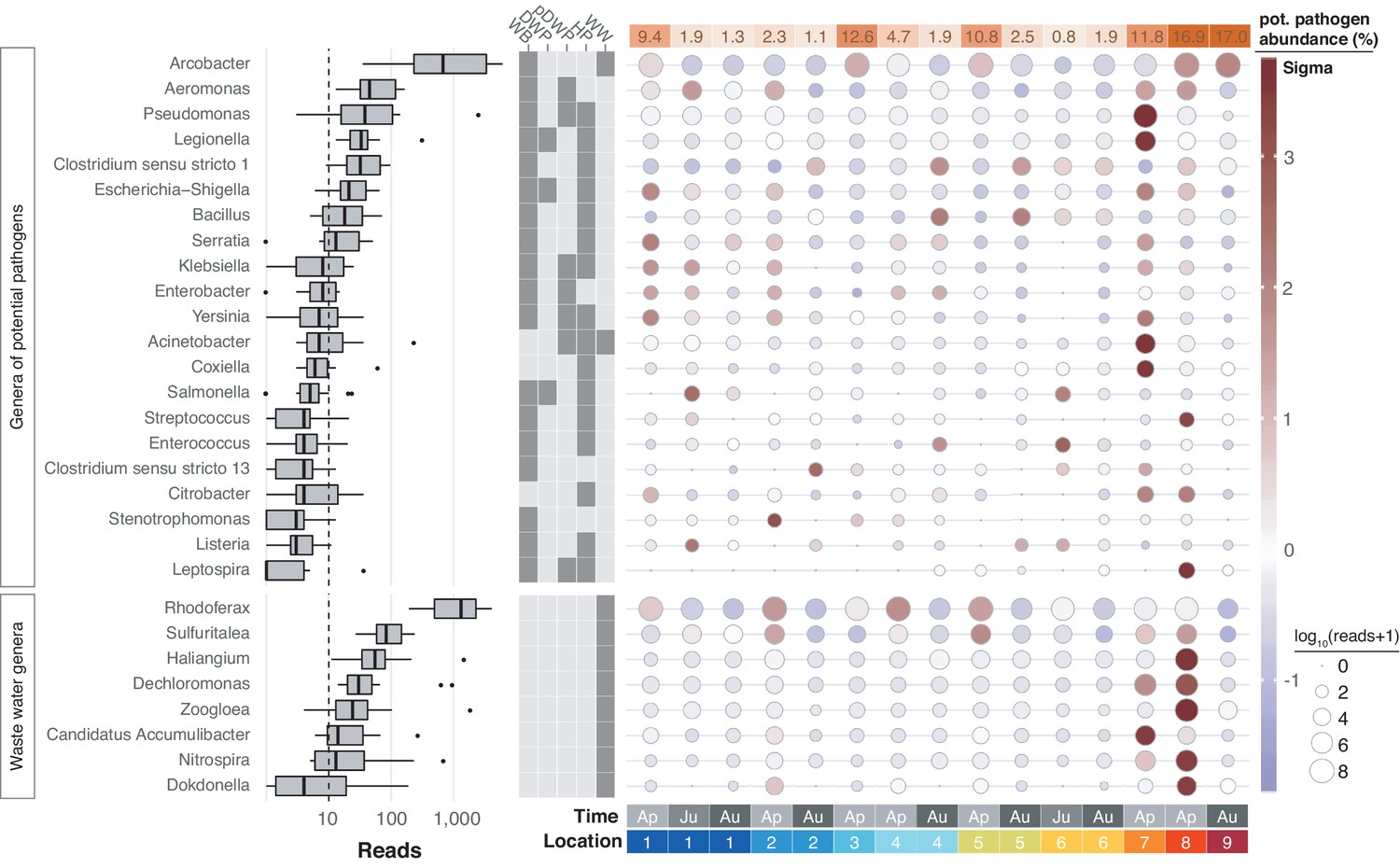
Potentially pathogenic and wastewater treatment related bacteria in the River Cam.
Boxplots on the left show the abundance distribution across locations per bacterial genus. Error bars represent Q1 – 1.5*IQR (lower), and Q3 + 1.5*IQR (upper), respectively; Q1: first quartile, Q3: third quartile, IQR: interquartile range. The central table depicts the categorisation of subsets of genera as waterborne bacterial pathogens (WB), drinking water pathogens (DWP), potential drinking water pathogens (pDWP), human pathogens (HP), and core genera from wastewater treatment plants (WW) (dark grey: included, light grey: excluded) (Supplementary file 3). The right-hand circle plot shows the distribution of bacterial genera across locations of the River Cam. Circle sizes represent overall read size fractions, while circle colours (sigma scheme) represent the standard deviation from the observed mean relative abundance within each genus.
Figure 8
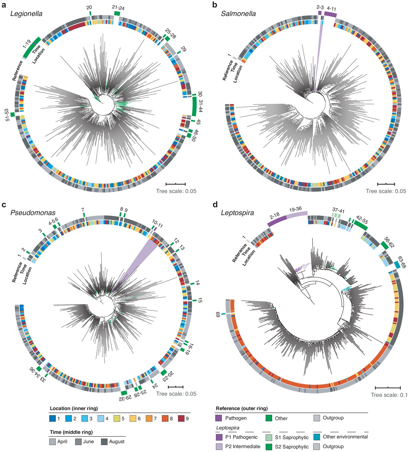
High-resolution phylogenetic clustering of candidate pathogenic genera in the River Cam.
Phylogenetic trees illustrating multiple sequence alignments of exemplary River Cam nanopore reads (black branches) classified as (a) Legionella, (b) Salmonella, (c) Pseudomonas, or (d) Leptospira, together with known reference species sequences ranging from pathogenic to saprophytic taxa within the same genus (coloured branches). Reference species sequences are numbered in clockwise orientation around the tree (Supplementary file 4). Nanopore reads highlighted in light violet background display close clustering with pathogenic isolates of (b) Salmonella spp. and (c) Pseudomonas aeruginosa.
Additional files
-
Supplementary file 1
Summary of samples and metadata.
(a) Sampling locations. (b) Environmental metadata by sample. (c) Environmental metadata by time point.
- https://cdn.elifesciences.org/articles/61504/elife-61504-supp1-v1.xlsx
-
Supplementary file 2
Summary of raw DNA, amplicon and sequencing yields.
(a) Water DNA extraction yields. (b) Full-length 16S PCR amplicon extraction yields. (c) Nanopore sequencing read metrics.
- https://cdn.elifesciences.org/articles/61504/elife-61504-supp2-v1.xlsx
-
Supplementary file 3
Summary of pathogen and wastewater bacterial genera tested.
(a-b) List of pathogen (a) and wastewater (b) candidate bacterial genera.
- https://cdn.elifesciences.org/articles/61504/elife-61504-supp3-v1.xlsx
-
Supplementary file 4
Summary of reference sequences for high-resolution pathogen mapping.
(a-d) References and NCBI accessions for Legionella (a), Salmonella (b), Pseudomonas (c), and Leptospira (d).
- https://cdn.elifesciences.org/articles/61504/elife-61504-supp4-v1.xlsx
-
Supplementary file 5
Summary of multi-species Leptospira quantifications by Taqman qPCR.
- https://cdn.elifesciences.org/articles/61504/elife-61504-supp5-v1.xlsx
-
Supplementary file 6
Summary of project costs.
(a) Basic sequencing workflow cost estimate. (b) Cost estimate per sample, based on a 12-plex MinION sequencing run. (c) Projected cost estimate per sample, based on a 100-plex MinION sequencing run.
- https://cdn.elifesciences.org/articles/61504/elife-61504-supp6-v1.xlsx
-
Supplementary file 7
Summary of full-length 16S primer sequences (5' - 3').
- https://cdn.elifesciences.org/articles/61504/elife-61504-supp7-v1.xlsx
-
Supplementary file 8
Summary of negative controls.
(a-c) Relative classification output per sample (%), sorted by negative control abundances in April (a), June (b), and August (c).
- https://cdn.elifesciences.org/articles/61504/elife-61504-supp8-v1.xlsx
-
Transparent reporting form
- https://cdn.elifesciences.org/articles/61504/elife-61504-transrepform-v1.pdf
Download links
A two-part list of links to download the article, or parts of the article, in various formats.
Downloads (link to download the article as PDF)
Open citations (links to open the citations from this article in various online reference manager services)
Cite this article (links to download the citations from this article in formats compatible with various reference manager tools)
Freshwater monitoring by nanopore sequencing
eLife 10:e61504.
https://doi.org/10.7554/eLife.61504


