Adaptation of spontaneous activity in the developing visual cortex
- Computation in Neural Circuits Group, Max Planck Institute for Brain Research, Germany
- School of Life Sciences Weihenstephan, Technical University of Munich, Germany
- Netherlands Institute for Neuroscience, Netherlands
- Center for Neurogenomics and Cognitive Research, Vrije Universiteit, Netherlands
Figures
Figure 1
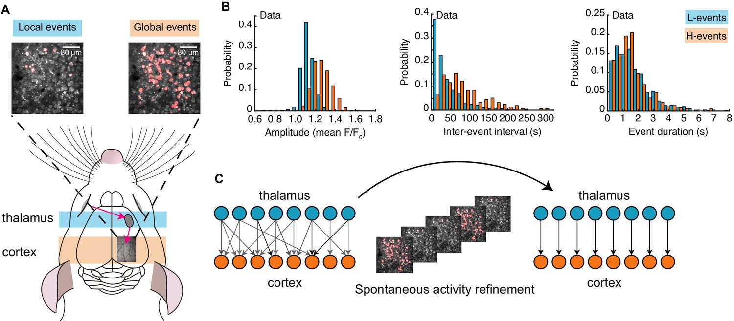
Spontaneous activity patterns in early postnatal development.
(A) Two distinct patterns of spontaneous activity recorded in vivo in the visual cortex of young mice before eye-opening (P8-10). Blue shading denotes local low-synchronicity (L-) events generated by the retina; orange shading denotes global high-synchronicity (H-) events generated by the cortex. Activated neurons during each event are shown in red. (B) Distributions of different event properties (amplitude, inter-event interval, and event duration). Amplitude was measured as changes in fluorescence, relative to baseline, F/F0. (C) Network schematic: thalamocortical connections are refined by spontaneous activity. The initially broad receptive fields with weak synapses evolve into a stable configuration with strong synapses organized topographically.
Figure 2

A network model of thalamocortical connectivity refinements.
(A) A feedforward network with an input layer of thalamic neurons connected to an output layer of cortical neurons by synaptic weights . (B) Properties of L- and H-events in the model (amplitude , inter-event interval and duration ) follow probability distributions extracted from data (Siegel et al., 2012) (see Table 1). (C) Initially weak all-to-all connectivity with a small topographic bias along the diagonal (left) gets refined by the spontaneous activity events (right). (D) Evaluating network refinement through receptive field statistics (see Materials and methods). We quantify two properties: (1) the receptive field size and (2) the topography, which quantifies on average how far away the receptive field center of each cortical cell (red dot) is from the diagonal (dashed gray line).
Figure 3 with 2 supplements
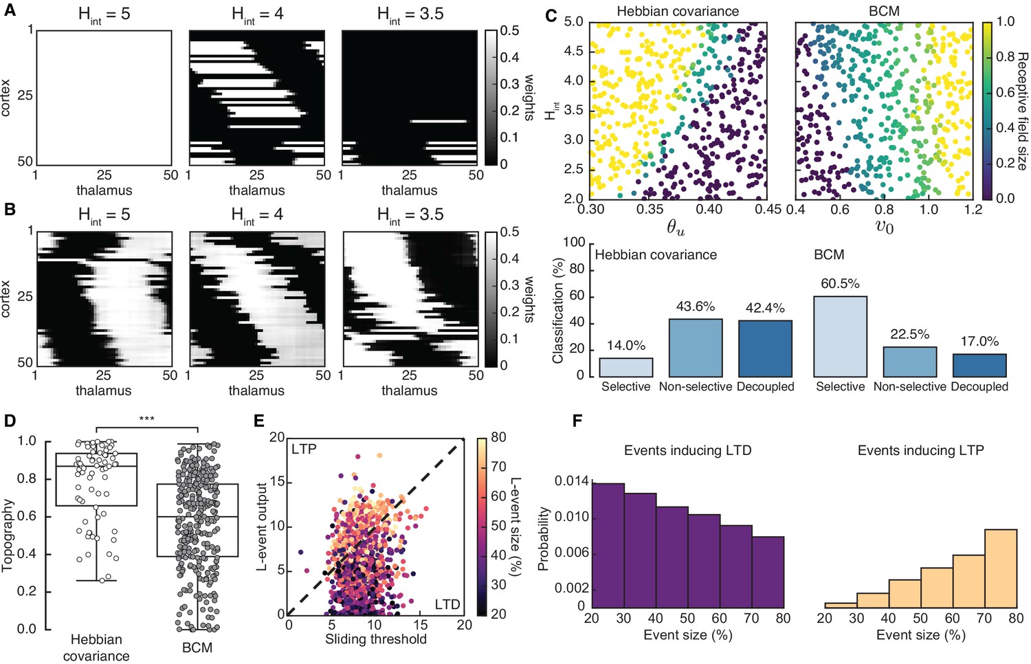
Spontaneous cortical events disrupt receptive field refinement.
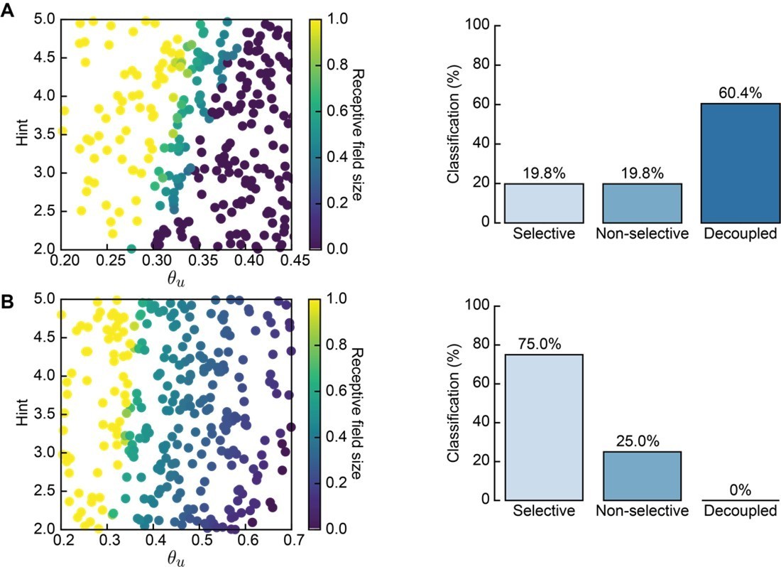
(A) Receptive fields generated by the Hebbian covariance rule with input threshold and decreasing . (B) Receptive fields generated by the BCM rule with target rate and decreasing . (C) Top: Receptive field sizes obtained from 500 Monte Carlo simulations for combinations of and for the Hebbian covariance rule (left) and and for the BCM rule (right). Bottom: Percentage of simulation outcomes classified as ‘selective’ when the average receptive field size is smaller than one and larger than 0, ‘non-selective’ when the average receptive field size is equal to 1, and ‘decoupled’ when the average receptive field size is 0 for the two rules. (D) Topography of receptive fields classified as selective in C. Horizontal line indicates median, the box is drawn between the 25th and 75th percentile, whiskers extend above and below the box to the most extreme data points that are within a distance to the box equal to 1.5 times the interquartile range and points indicate all data points. Distributions are significantly different (***) as measured by a two-sample Kolmogorov-Smirnov test ( selective outcomes for each rule out of 500; ; D = 0.45). (E) The response of a single cortical cell to L-events of different sizes (color) as a function of the sliding threshold for the BCM rule with and . The cell’s incoming synaptic weights from presynaptic thalamic neurons undergo LTP or LTD depending on L-event size. (F) Probability of L-event size contributing to LTD (left) and LTP (right) for the BCM rule with the same parameters as in E.
Figure 3—figure supplement 1
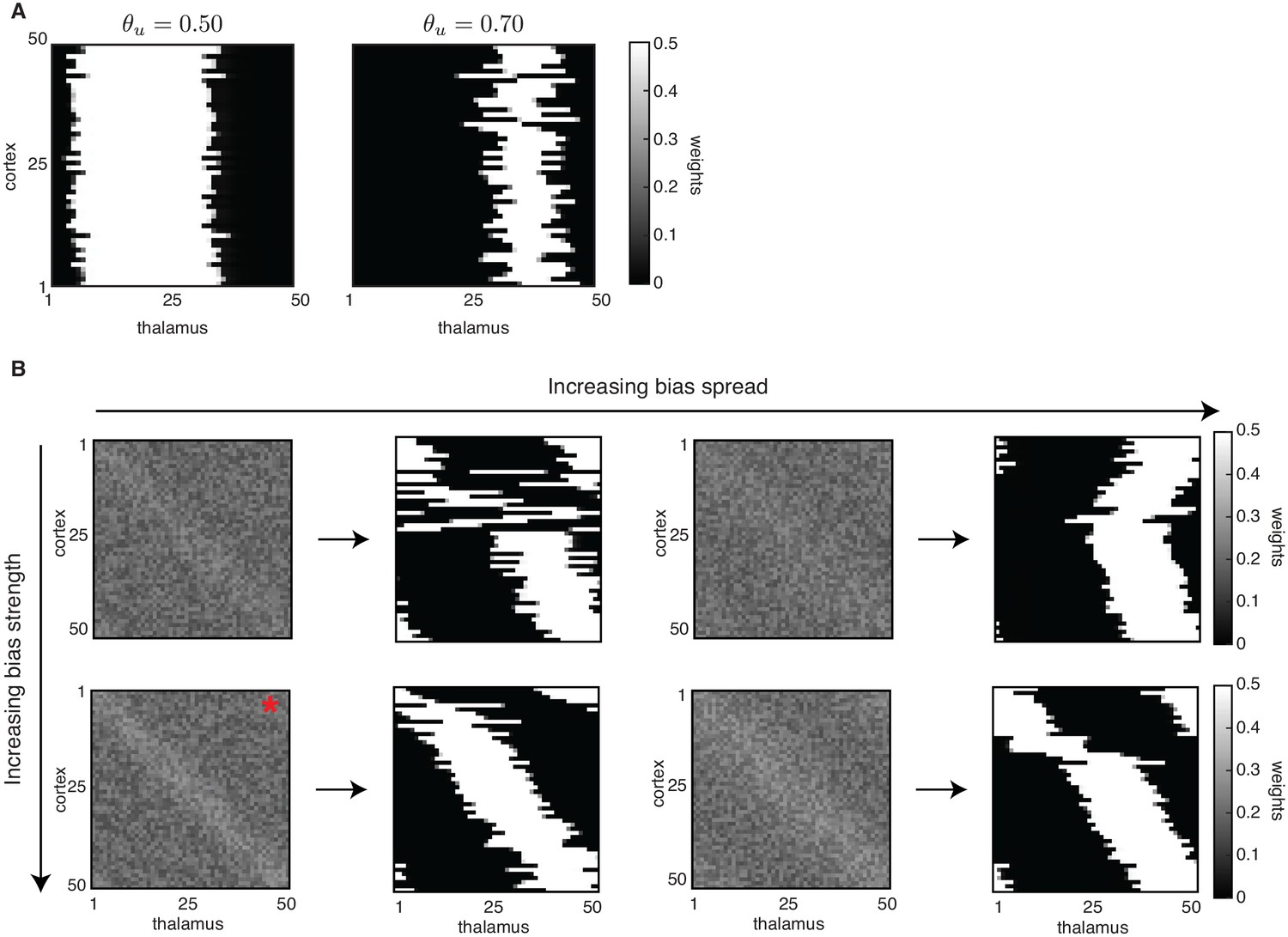
Effect of initial bias on receptive field refinements and topography.
Effect of initial bias on receptive field refinements and topography. (A) Without the weak bias along the diagonal, selectivity is achieved so that each cortical cell is connected to a few thalamic inputs; however, the same set of input neurons innervates all cortical neurons. Receptive fields were generated with the Hebbian covariance rule, but similar outcomes are obtained with the BCM rule. (B) Each pair of plots shows the initial biased connectivity (left) and the final outcome of the simulation (right) for one combination of bias spread and bias strength. Top: Weaker bias strength (relative to the nominal one used in the paper simulations) with increasing spread. Bottom: Nominal bias strength with increasing spread. Initial conditions used in the paper correspond to the bottom left panel (marked with a red asterisk). Simulations of the Hebbian learning rule with an input threshold and only L-events. We show bias strength and bias spread .
Figure 3—figure supplement 2
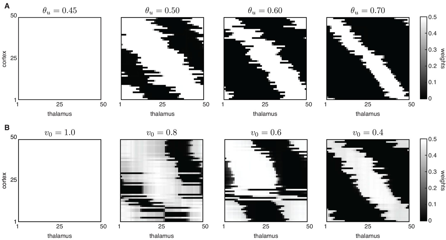
Peripheral L-events generate robust receptive field refinement in the absence of H-events.
Peripheral L-events generate robust receptive field refinement in the absence of H-events. (A) Receptive fields generated by the Hebbian covariance rule with only L-events and varying input threshold . (B) Receptive fields generated by the BCM rule with only L-events and varying target output target rate v0.
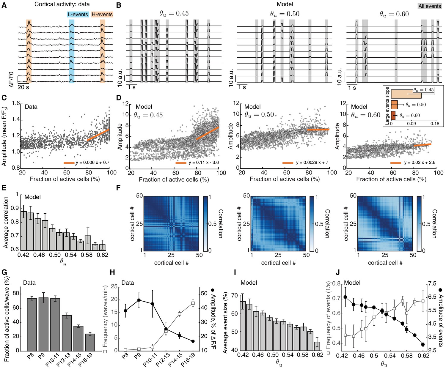
Figure 4
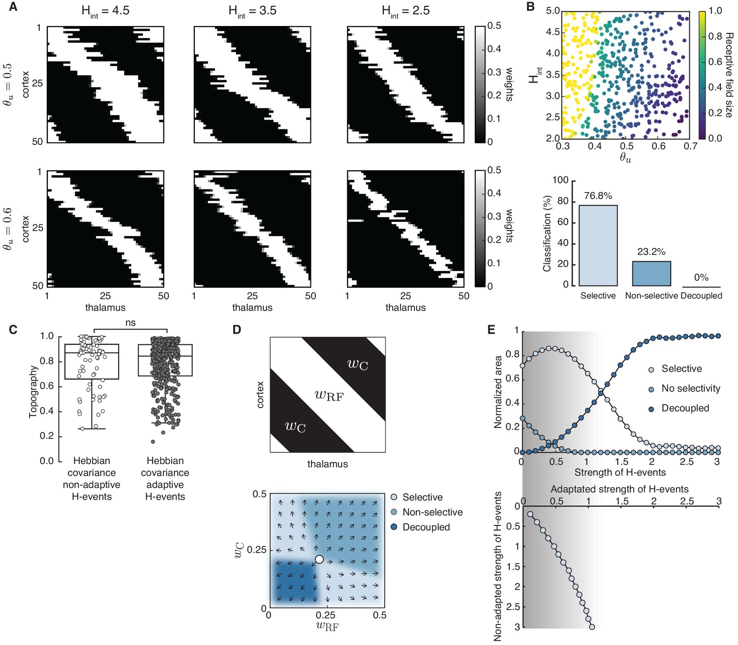
Adaptive cortical events refine thalamocortical connectivity.
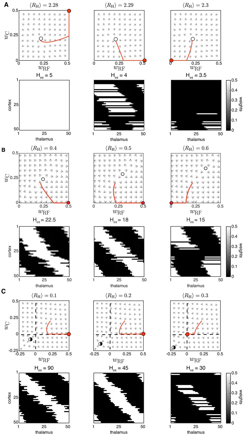
(A) Receptive field refinement with adaptive H-events and different H-inter-event-intervals, . Top: ; bottom: . (B) Receptive field sizes from 500 Monte Carlo simulations for combinations of and . Bottom: Percentage of simulation outcomes classified as ‘selective’ when the average receptive field size is smaller than one and larger than 0, ‘non-selective’ when the average receptive field size is equal to 1, and ‘decoupled’ when the average receptive field size is 0 for the two rules. (C) Topography of receptive fields classified as selective in B. Horizontal line indicates median, the box is drawn between the 25th and 75th percentile, whiskers extend above and below the box to the most extreme data points that are within a distance to the box equal to 1.5 times the interquartile range and points indicate all data points. Distributions are not significantly different (ns) as measured by a two-sample Kolmogorov-Smirnov test ( selective outcomes for each rule out of 500; ; D = 0.45). (D) Top: Reduction of the full weight dynamics into two dimensions. Two sets of weights were averaged: those which potentiate and form the receptive field, , and the complementary set of weights that depress, . Bottom: Initial conditions in the reduced two-dimensional phase plane were classified into three outcomes: ‘selective’, ‘non-selective’, and ‘decoupled’. We sampled 2500 initial conditions which evolved according to Equation 16 until the trajectories reached one of the selective fixed points, and , or resulted in no selectivity either because both weights depressed to or potentiated to . The normalized number of initial coordinates generating each region can be interpreted as the area of the phase plane that results in each outcome. (E) Top: Normalized area of the phase plane of the reduced two-dimensional system that resulted in ‘selective’, ‘non-selective’, and ‘decoupled’ outcomes for as a function of H-event strength. The darker shading indicates ranges of non-adapted H-event strength where the selectivity area is maximized. Bottom: The corresponding adapted strength of H-events was calculated in simulations with adaptive H-events and plotted as a function of the nominal, non-adapted strength of H-events. The range of adapted H-event strengths (bottom) corresponds to the range of non-adaptive values that maximize the selectivity area (top). Each point shows the average over 10 runs and the bars the standard deviation (which are very small).
Figure 5 with 3 supplements

Spontaneous events in developing cortex adapt to recent activity.
(A) Calcium trace of a representative recording with L- (blue) and H-events (orange) (Siegel et al., 2012). (B) The amplitude of an H-event shown as a function of the aggregate amplitude of preceding L- and H-events up to s before it, scaled by an exponential kernel with a decay time constant of 1000 s ( events from nine animals). Animals with fewer than 12 H-events preceded by activity within were excluded from this analysis (see Materials and methods). The Pearson correlation coefficient is , CI . Red line indicates regression line with 95% confidence bounds as dashed lines. (C) Schematic of the postulated adaptation: A weak (strong) H-event is more likely to be preceded by weak (strong) spontaneous events.
Figure 5—figure supplement 1
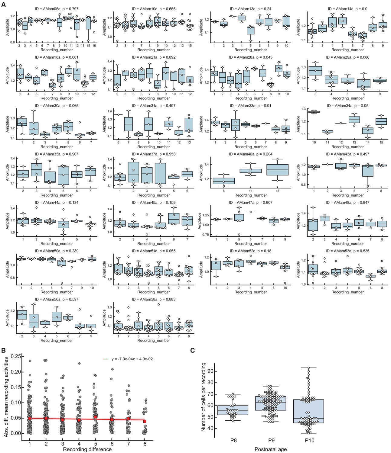
Fluctuations in cortical activity cannot generate correlations between event amplitude and average preceding activity.
Fluctuations in cortical activity cannot generate correlations between event amplitude and average preceding activity. (A) Spontaneous events have similar mean amplitudes across consecutive recordings (each ∼5 min long) in the same animal (3–14 recordings in 26 animals separated by <5 min due to experimental constraints on data collection). Each plot corresponds to one animal, where each boxplot contains the event amplitudes (both L- and H-events) from each recording. Horizontal line indicates median, the box is drawn between the 25th and 75th percentile, whiskers extend above and below the box to the most extreme data points that are within a distance to the box equal to 1.5 times the interquartile range and points indicate all data points. p-Values of one-way ANOVA tests of the event amplitudes across recordings are shown for each animal. (B) Absolute difference in the mean event amplitude as a function of time between recordings. Mean values of each recording difference shown as red squares. The values follow the same distribution (Kruskal-Wallis test p=0.41). The slope of the linear regression fit (red) is very close to 0, confirming that no clear trend of increasing/decreasing activity exists across recordings. (C) Number of cells per recording, grouped by different postnatal ages. Horizontal line indicates median, the box is drawn between the 25th and 75th percentile, whiskers extend above and below the box to the most extreme data points that are within a distance to the box equal to 1.5 times the interquartile range and points indicate all data points.
Figure 5—figure supplement 2
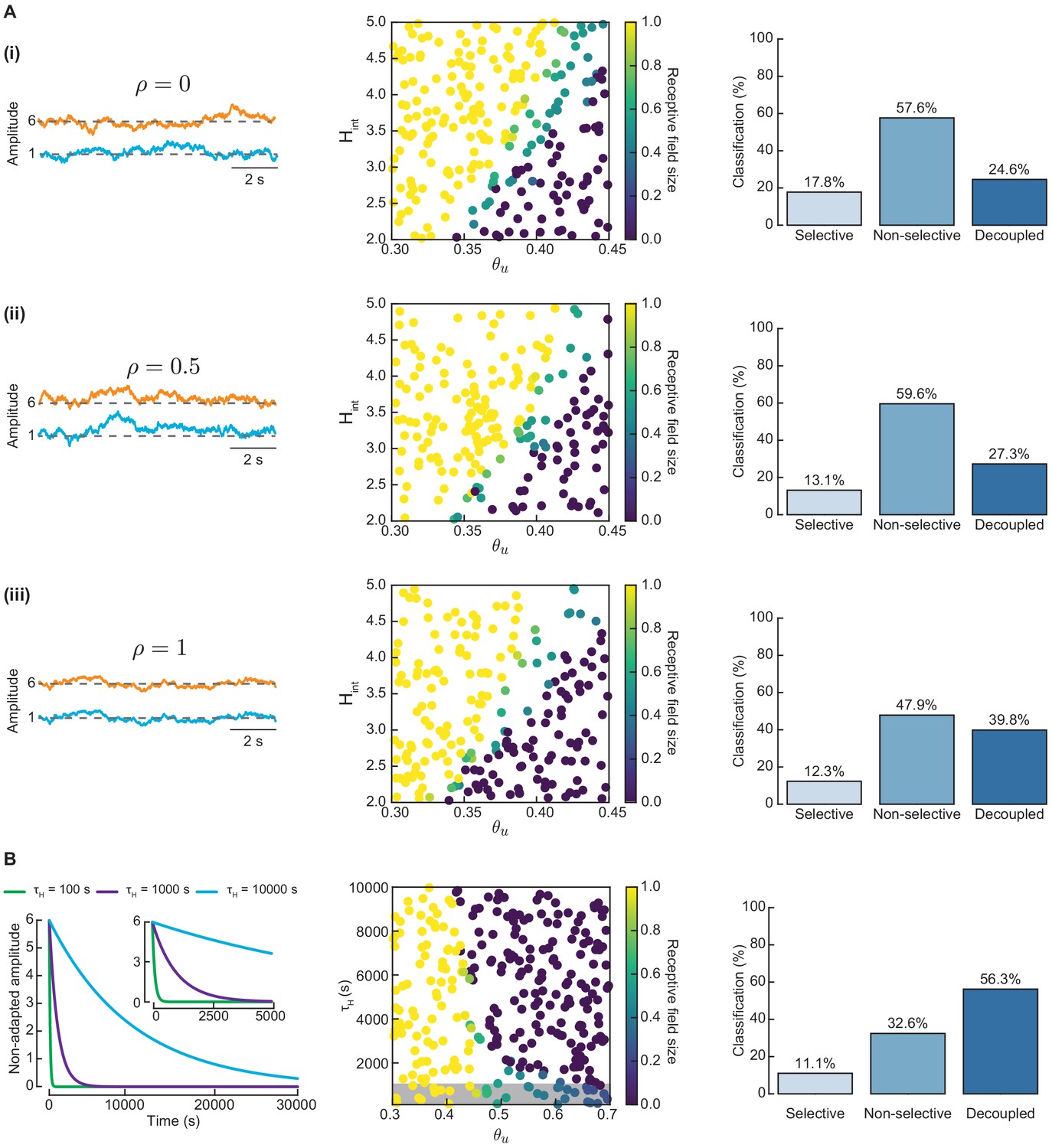
Long-term fluctuations in the amplitudes of L- and H-events cannot guide proper network refinement.
Long-term fluctuations in the amplitudes of L- and H-events cannot guide proper network refinement. (A) Correlated fluctuations in the amplitudes of L- and H-events are not sufficient to guide proper network refinement. Left: Amplitudes of L- (blue) and H-events (orange) follow Ornstein-Uhlenbeck processes of different correlation strengths, ρ: (i) uncorrelated (), (ii) intermediate correlation (), and (iii) perfect correlation (). We simulated the model with non-adaptive H-events with these different correlation strengths. Middle: Receptive field sizes for 200 Monte Carlo simulations in the same parameter space of and as the manuscript. Right: Simulations were classified into three possible outputs: selective, non-selective, and decoupled networks. (B) A top-down signal which imposes an exponential decay of H-event amplitudes during development (independent of ongoing network activity) enhances receptive field refinement only if the decay is very fast. Left: Exponential decay of non-adaptive H-event amplitudes. We simulated the model with non-adaptive H-events with different amplitude decay time constants s. The inset shows a detail of the beginning of the simulation. Middle: Receptive field sizes for 300 Monte Carlo simulations for non-adaptive H-events with exponentially decaying H-event amplitudes in the range s and input thresholds in the range . The gray box indicates simulations with very fast decaying amplitudes ( s) that generate refined receptive fields. Right: Simulations classified into three possible outputs: selective, non-selective, and decoupled networks.
Figure 5—figure supplement 3
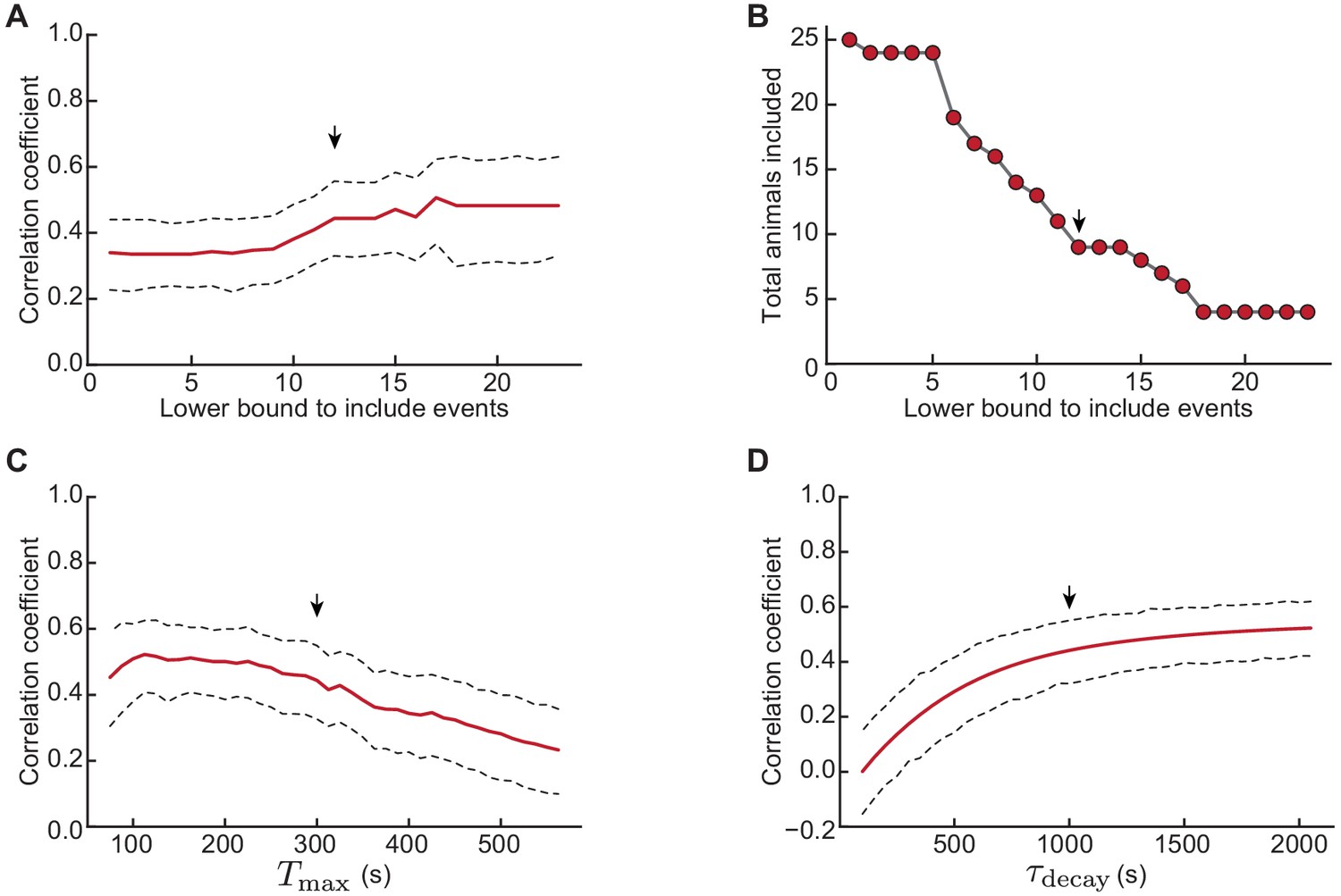
Robustness of correlation under variations in the inclusion criteria, and .
Robustness of correlation under variations in the inclusion criteria, and . (A) Correlation coefficient between H-event amplitude and aggregate scaled amplitude of preceding events for an increasing lower bound in the number of H-events necessary to include an animal in the analysis (see Materials and methods, s and s fixed). 95% confidence interval (dashed lines) computed through bootstrap regression (see Materials and methods). (B) Corresponding number of animals satisfying the lower bound criteria in A. (C) Correlation coefficient between H-event amplitude and aggregate scaled amplitude of preceding events for varying windows of integration (lower bound to include H-events fixed at 12, s). (D) Correlation coefficient between H-event amplitude and aggregate scaled amplitude of preceding events as a function of the exponential decay time constant (lower bound to include H-events fixed at 12, s). The small vertical arrows indicate the parameters of the analysis in Figure 5, namely a minimuml of 12 events per animal, s, s.
Figure 6
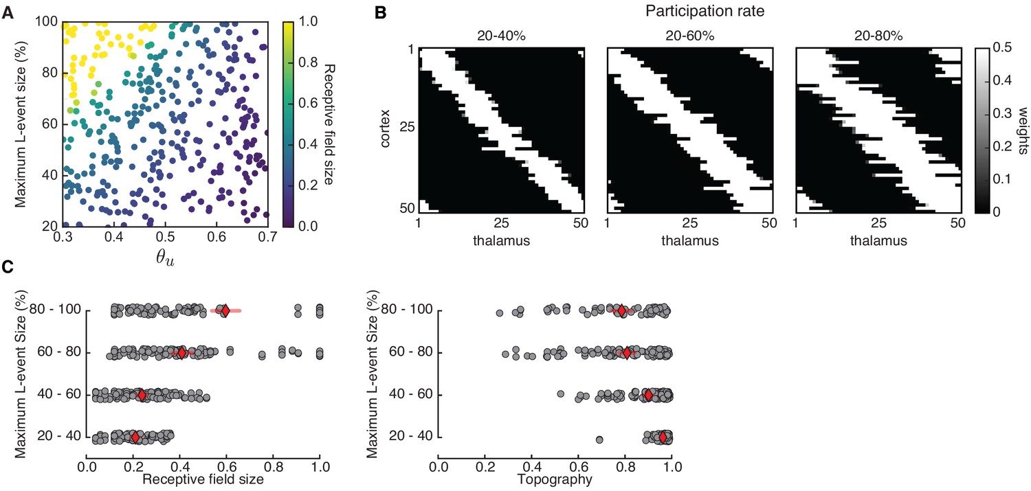
Receptive field refinement depends on the properties of L-events.
(A) Receptive field sizes from 500 Monte Carlo simulations for different sizes of L-events where the minimum participation rate was 20%, and the maximum participation rate was varied. The input threshold was taken from the range , while the adaptive H-events had a fixed inter-event-interval . (B) Individual receptive fields for different L-event maximum participation rates and . As the upper bound of the participation rate progressively increases from 40% to 80%, receptive fields get larger. (C) Left: Receptive field sizes from A binned according to the maximum L-event size. Right: Corresponding topography of selective receptive fields for different sizes of L-events. Diamonds in red indicate the mean, while horizontal bars indicate the 95% confidence interval.
Figure 7 with 1 supplement
Adaptive H-events promote sparsification of cortical activity during development.
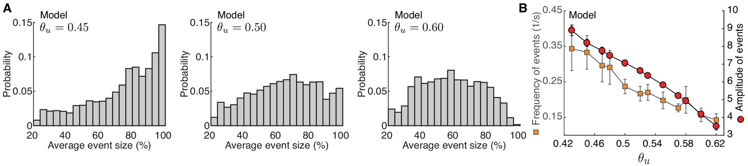
(A) Spontaneous activity in the mouse visual cortex recorded in vivo at P8-10 (Siegel et al., 2012). Each activity trace represents an individual cortical cell. Blue and orange shading denotes L-events and H-events, respectively, as identified by Siegel et al., 2012. (B) Sample traces of cortical activity for different values of (as a proxy for developmental age). Gray shading denotes all events detected in our networks. (C) Amplitude vs. participation rate plot from the data (Siegel et al., 2012). The regression line for the amplitude vs. participation rate in H-events has a positive slope. (D) Amplitude vs. participation rate plots from the model, for different values of . Inset: The regression line for the amplitude vs. participation rate in large events with greater than 80% participation rate has a slope that decreases with . Error bars represent standard deviation. (E) Correlation between cortical neurons decreases as a function of the input threshold in the model, a proxy for developmental time. (F) Correlation matrices of simulated cortical neuron activity corresponding to D. (G,H). Event sizes and the relationship between frequencies (open squares) and amplitudes (filled circles) of spontaneous events at different postnatal ages (data reproduced from Rochefort et al., 2009). Error bars represent standard error of the mean (number of animals used at each age is provided in the original reference). (I) Spontaneous event sizes as a function of the input threshold . (J) Frequencies (squares) and amplitudes (circles) of events with 20–80% participation rate in the model at different input thresholds. Error bars represent the standard error of the mean of 10 simulations.
Figure 7—figure supplement 1
Developmental event sparsification in the model.
Developmental event sparsification in the model. (A) Distribution of spontaneous event sizes for the different input thresholds in the model as Figure 7D. (B) Frequencies (squares) and amplitudes (circles) of events with greater than 80% participation rate in the model at different input thresholds (abscissa). These events are suppressed both in amplitude and frequency at higher input threshold . Error bars represent the standard deviation of 10 simulations.
Appendix 1—figure 1

Receptive field size depends on L-event properties and learning rule input threshold in the absence of H-events.
(A) Receptive field sizes from 500 Monte Carlo simulations for combinations of L-event maximum participation rate and input threshold, . For all simulations, the L-event minimum participation rate was fixed at 20%. The contour plots of receptive field sizes were obtained using the analytical approach (Equation 23). (B) Example receptive fields for different L-event maximum participation rates and . Smaller events recruiting only 20–40% of the input neurons generate very refined receptive fields. As the upper bound of the participation rate progressively increases from 40% to 80%, receptive fields get larger.
Appendix 1—figure 2

Eigenvalues and eigenvectors of weight dynamics predict receptive field refinement.
(A) The input correlation matrix . (B) The modified covariance matrices for different input thresholds, . (C) Two thresholds, and , define three different dynamical regions in the spectrum of , delineated by the horizontal red dashed lines: (i) , (ii) , and (iii) . The row-sum eigenvalue in each case is given by the yellow star, while the remaining eigenvalues are shown as gray circles. (D) Dominant eigenvectors corresponding to each region in C. Inset: fixed points corresponding to each region: (i), (ii) unstable node (open circles); (iii) saddle node (half-open circle).
Appendix 1—figure 3
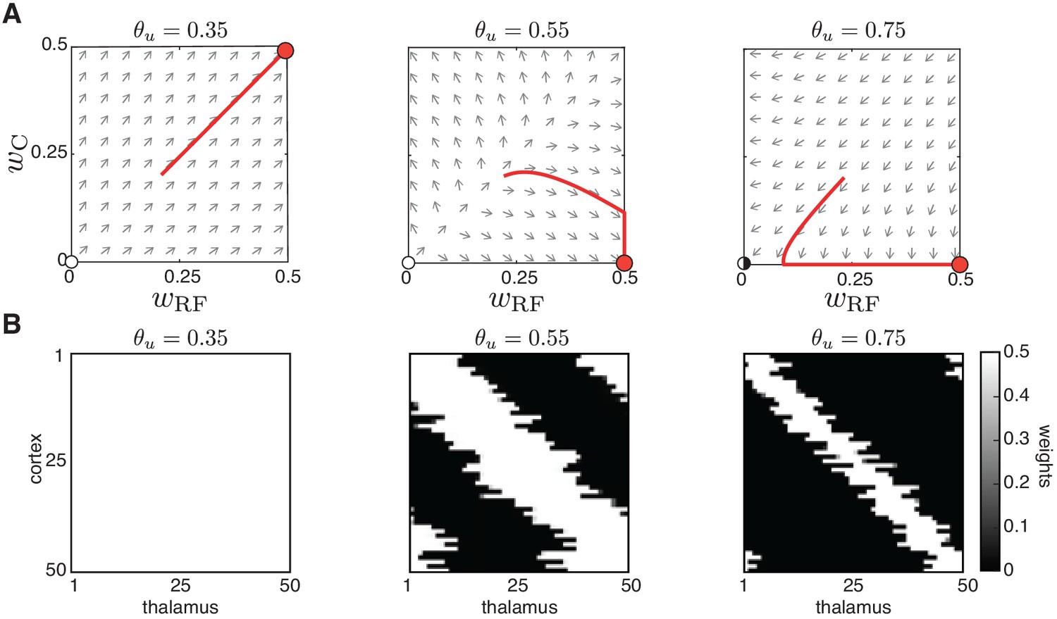
Peripheral L-events generate robust receptive field refinement.
(A) The reduced two-dimensional weight dynamics in the phase plane with the same as Appendix 1–figure 2B and D. For each plane, the red trajectory depicts the weight evolution from an initial condition where until the weights’ upper bound (). Left: and , resulting in no selectivity. Middle and right: and , resulting in selectivity and receptive field refinement. (B) Simulation results for the same input thresholds of Appendix 1–figure 2B,D for the full 50-dimensional system.
Appendix 1—figure 4
Spontaneous cortical H-events disrupt receptive field refinement.
(A) Top: Phase planes of the reduced two-dimensional system for input threshold (region i) and increasing strength of cortical events with an example trajectory (red). Selectivity can only be observed for fine-tuned . The fixed point (open circle), an unstable node, has moved to the first quadrant. Bottom: Simulations of receptive field development with the same parameters where was progressively reduced (this is the same set of parameters as shown in Figure 3A). (B) Top: Phase planes for (region ii) and increasing with an example trajectory (red). The unstable node (open circle) moves from the origin to the first quadrant as increases. Bottom. Simulations with the same parameters where was progressively reduced. (C) Top: Phase planes for (region iii) show the transition from selective receptive fields to cortical decoupling in response to increasing . The fixed point (half-open circle), now a saddle node because , has moved away from the origin to the third quadrant. Bottom: Simulations with the same parameters with very infrequent H-events where was progressively reduced.
Author response image 1
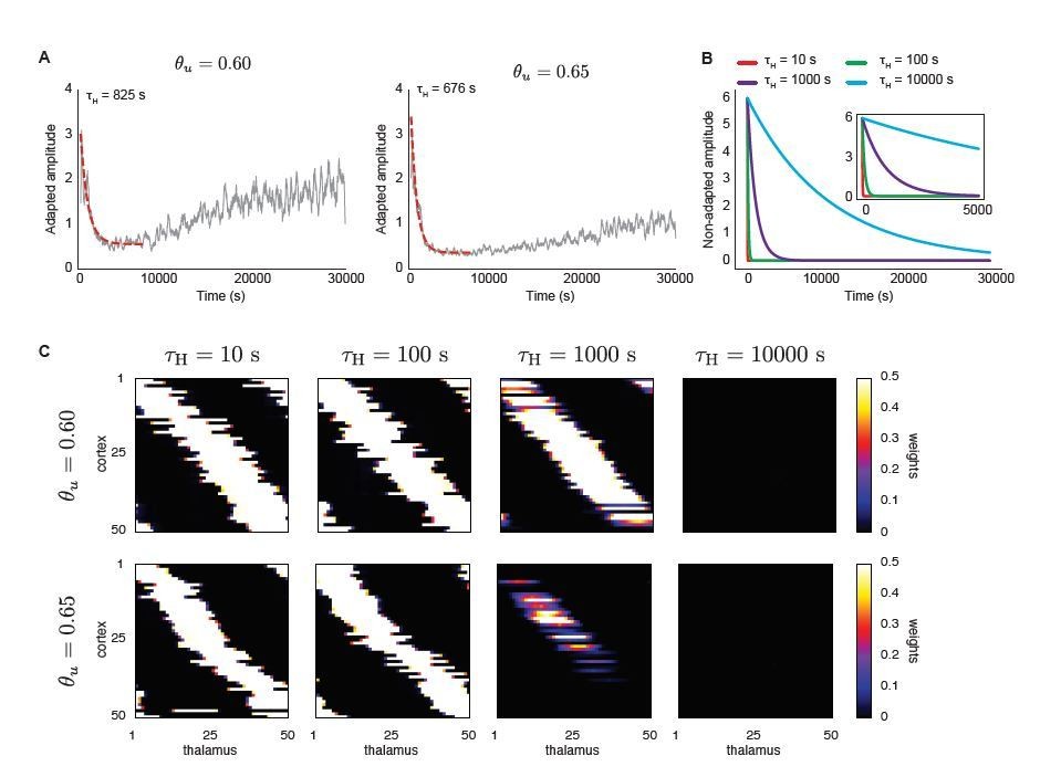
A top-down signal imposes exponential decay of H-event amplitudes during development (independent of ongoing network activity) enhances receptive field refinement only if the decay is very fast.
A. Average amplitudes of adaptive H-events as a function of simulation time for two input thresholds in the Hebbian learning rule, θu = 0.6 and θu = 0.65. To determine the decay time constants used in B and C, an exponential decay function was fitted to the initial decay of amplitude, with fitted decay time constants τH = 825 s and τH = 676 s, respectively. B. Using the range of time constants from A, we simulated the model with non-adaptive H-events. Their amplitudes decayed exponentially with different decay time constants (τH = {10,100,1000,10000} s). The inset shows a detail of the beginning of the simulation. C. Final receptive fields for non-adaptive H-events with exponentially decaying amplitudes as in B for the two different input thresholds.
Author response image 2
Receptive field statistics for a different distribution of L- and H-event sizes (20–70% and 70–100% participation rates, respectively).
A. 300 Monte Carlo simulations with non-adaptive H-events: receptive field size (left) and proportion of simulations that resulted in selective, non-selective and decoupled receptive fields (right). Compare to Figure 3C. B. Same as A for adaptive H-events in the same range of parameters. Compare to Figure 4B.
Tables
Table 1
List of parameters used in the model unless stated otherwise.
| Name | Value/Distribution | Description |
|---|---|---|
| Network | ||
| 50 | Number of thalamic neurons | |
| 50 | Number of cortical neurons | |
| 50,000 | Simulation length [s] | |
| Weights | ||
| U(0.15,0.25) | Range of initial weights (U: uniform dist.) | |
| 0.05 | Amplitude of Gaussian bias | |
| 4 | Spread of Gaussian bias | |
| 0.5 | Weight saturation limit | |
| L-events | ||
| 1.0 | Amplitude (equivalently, binary neuron) | |
| U(20%,80%) | Percentage of thalamic cells activated | |
| Mean duration [s] (: Gaussian dist.) | ||
| Exp(1.5) | Mean inter-event interval [s] (Exp: exponential dist.) | |
| H-events | ||
| Amplitude | ||
| U(80%,100%) | Percentage of cortical cells activated | |
| Mean duration [s] | ||
| Gamma(3.5, 1.0) | Mean inter-event interval [s] (Gamma: Gamma dist.) | |
| Time constants | ||
| 0.01 | Membrane time constant [s] | |
| 500 | Weight-change time constant for Hebbian covariance rule [s] | |
| 1000 | Weight-change time constant for BCM rule [s] | |
| 20 | Output threshold time constant for BCM rule [s] | |
| 1 | Adaptation time constant [s] | |
Additional files
Download links
A two-part list of links to download the article, or parts of the article, in various formats.
Downloads (link to download the article as PDF)
Open citations (links to open the citations from this article in various online reference manager services)
Cite this article (links to download the citations from this article in formats compatible with various reference manager tools)
Adaptation of spontaneous activity in the developing visual cortex
eLife 10:e61619.
https://doi.org/10.7554/eLife.61619


