Figures and data in Decoding the physical principles of two-component biomolecular phase separation

Figures
Tables
Additional files

25 figures, 3 tables and 1 additional file

Figures

Figure 1

Download asset Open asset

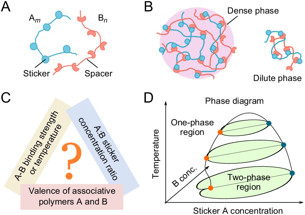
Phase behavior of sticker and spacer associative polymers.

(A) Schematic of multivalent associative polymers. Each polymer consists of complementary domains (stickers) connected by flexible linkers (spacers). A and B denote the polymer type and m and n denote their valences (number of stickers). (B) Association of stickers drives phase separation, leading to the formation of a dense, network phase coexisting with a dilute phase of small oligomers (depicted by a dimer). (C) The phase diagram depends on variety of biologically tunable parameters. In this study, we focus on the effects of sticker-sticker binding strength, sticker:sticker concentration ratio (i.e. stoichiometry), and polymer valences. (D) Schematic of a representative 3D phase diagram of an $A_{n} : B_{n}$ system as a function of temperature (inverse of binding strength) and A and B sticker concentrations. The dilute-phase concentration displays anomalous dependence on the binding strength and sticker concentrations in the strong binding regime. This is the ‘magic-ratio’ effect which we explore here in detail.

Figure 2

Download asset Open asset

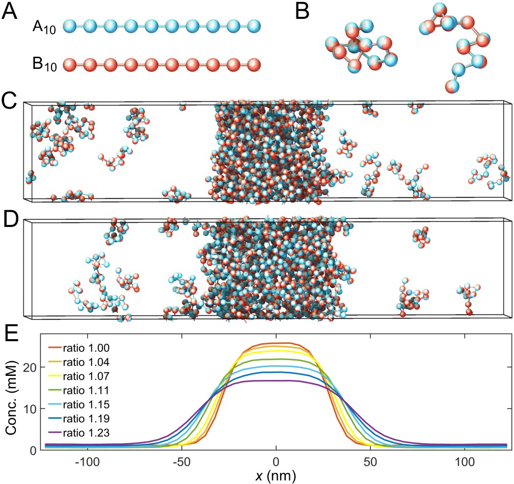
Coarse-grained molecular-dynamics simulations of two-component multivalent associative polymers.

(A) The system consists of two types of polymers A (blue) and B (red) of varying lengths and concentrations. Depicted are A and B polymers of length 10, denoted as A₁₀ and B₁₀. Each polymer is modeled as a linear chain of spherical particles connected by harmonic bonds. Stickers of different types interact pairwisely through an attractive potential, while repulsion between stickers of the same type prevents them from overlapping and thus ensures one-to-one binding of stickers of different types (see Appendix 1 for details). (B) Snapshots of dimers formed by A₁₀ and B₁₀ with one-to-one bonds. (C) Snapshot of a simulation with 125 A₁₀ and 125 B₁₀ polymers. The system phase separates into a dense phase (middle region) and a dilute phase (two sides) in a 250 nm×50 nm×50 nm simulation box with periodic boundary conditions. (D) Same as C but with 138 A₁₀ and 112 B₁₀ polymers, yielding an overall sticker concentration ratio 1.23. (E) Sticker concentration profiles of A₁₀:B₁₀ systems at various overall sticker stoichiometries (total global sticker concentration fixed at 6.64 mM), each with the center of the dense phase aligned at $x = 0$ and averaged over time and over ten simulation repeats (see Appendix 1). All simulations performed in LAMMPS (Plimpton, 1995).

Figure 3

Download asset Open asset

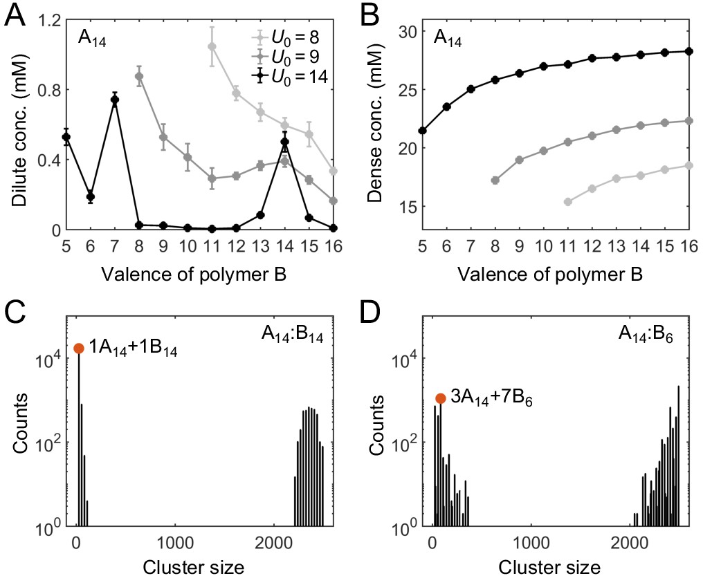
Simulations of associative polymers reveal a magic-number effect with respect to relative valence.

Total sticker concentrations (type A plus type B) in (A) dilute and (B) dense phases for simulated polymer systems at different binding strengths. U₀ denotes the depth of the potential well, in units of $k_{B} T$ (see Appendix 1 for details). The valence of polymer A is 14, and the valence of polymer B ranges from 5 to 16. Global sticker stoichiometry is one and total global sticker concentration is 6.64 mM. Histograms of cluster size in (C) A₁₄:B₁₄ and (D) A₁₄:B₆ systems, for $U_{0} = 14$ . ‘Counts’ refer to number of clusters. Cluster size is measured in stickers. Red dots indicate the dominant oligomer in the dilute phase.

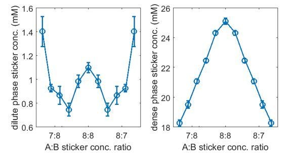
Figure 4

Download asset Open asset

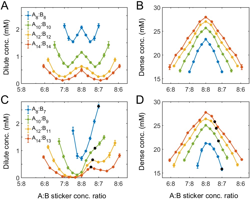
Simulations of associative polymers reveal a magic-ratio effect with respect to polymer stoichiometry.

Sticker concentrations in (A) dilute and (B) dense phases for equal polymer length systems (i.e. $A_{n} : B_{n}$ ) at different global sticker stoichiometries. Sticker concentrations in (C) dilute and (D) dense phases for systems where polymer B is one sticker shorter than polymer A (i.e. $A_{n} : B_{n - 1}$ ) at different global sticker stoichiometries; black dots indicate cases where the number of polymers of each type is the same. Interaction strength $U_{0} = 14$ and total global sticker concentration 6.64 mM.

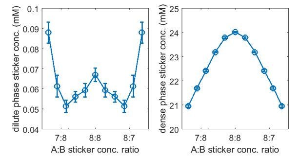
Figure 5

Download asset Open asset

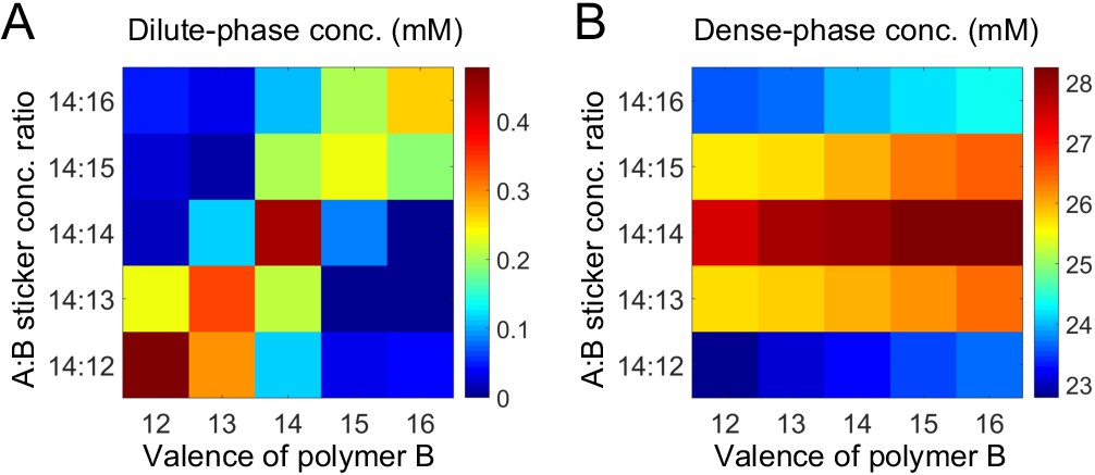
Simulations of associative polymers reveal a magic-ratio effect.

Sum of concentrations of stickers A and B in (A) dilute and (B) dense phases for systems A₁₄:B_12-16 at global sticker stoichiometries 14:12-16. Parameters: interaction strength $U_{0} = 14$ and total global sticker concentration 6.64 mM.

Figure 6

Download asset Open asset

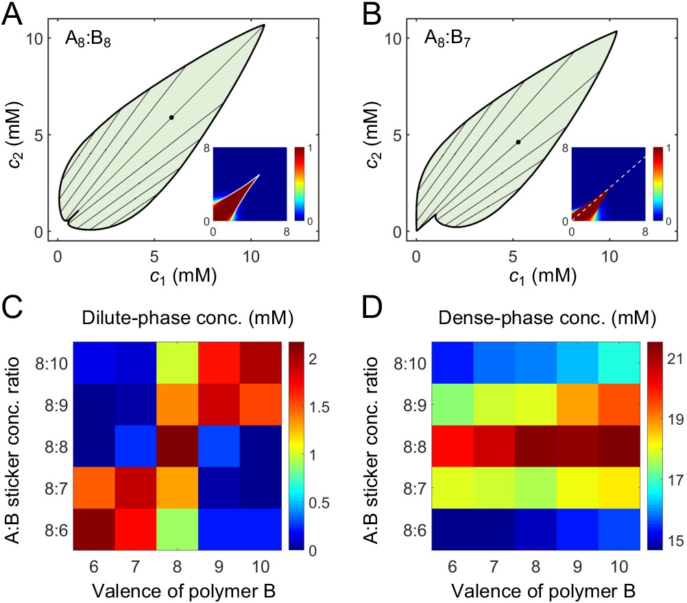
A dimer-gel theory predicts the magic-ratio effect.

Phase diagrams of (A) A₈:B₈ and (B) A₈:B₇ systems: one-phase region white, two-phase region green. The dilute- and dense-phase concentrations are connected by representative tie lines. The tie line along the direction of equal polymer stoichiometry is denoted with a black dot. Insets: fraction of stickers in dimers for (A) A₈:B₈ and (B) A₈:B₇ systems. White curve in A inset is the transition boundary between dimer- and independent bonds-dominated regions predicted by c_s. Dashed white line in (B) inset denotes equal polymer stoichiometry. Sticker concentrations in (C) dilute and (D) dense phases for systems A₈:B_6-10 at global sticker stoichiometries 8:6-10. The total global sticker concentration is the same as in simulations, 6.64 mM. For details see Appendix 2. Parameters: $v_{b} = 9 \times 10^{- 2} {mM}^{- 1}$ , $w_{b} = 7 \times 10^{- 3} {mM}^{- 2}$ , $K_{b} = 3.8 \times 10^{- 3} mM$ , and $K_{d}$ values in Appendix 1—table 3.

Appendix 1—figure 1

Download asset Open asset

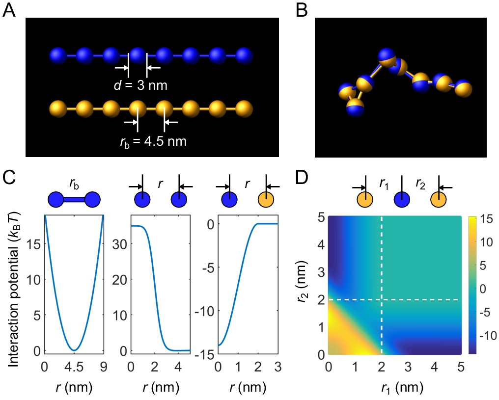
Coarse-grained molecular-dynamics simulations of two-component multivalent associative polymers.

(A) Polymers are modeled as linear chains of spherical particles connected by harmonic bonds. Depicted are A₈ (blue) and B₈ (yellow). (B) Snapshot of a dimer of A₈ and B₈ formed in the strong-binding regime. (C) Neighboring stickers in a polymer are connected through a harmonic potential (*left*). Stickers of the same type interact pairwisely through a repulsive potential (*middle*). Stickers of different types interact pairwisely through an attractive potential (*right*). (D) Interaction energy between three particles (one A and two B stickers) as a function of their separation distances. Simultaneous binding of two B stickers to one A sticker is energetically highly disfavored (lower left region) compared to one-to-one binding (dark blue regions).

Appendix 1—figure 2

Download asset Open asset

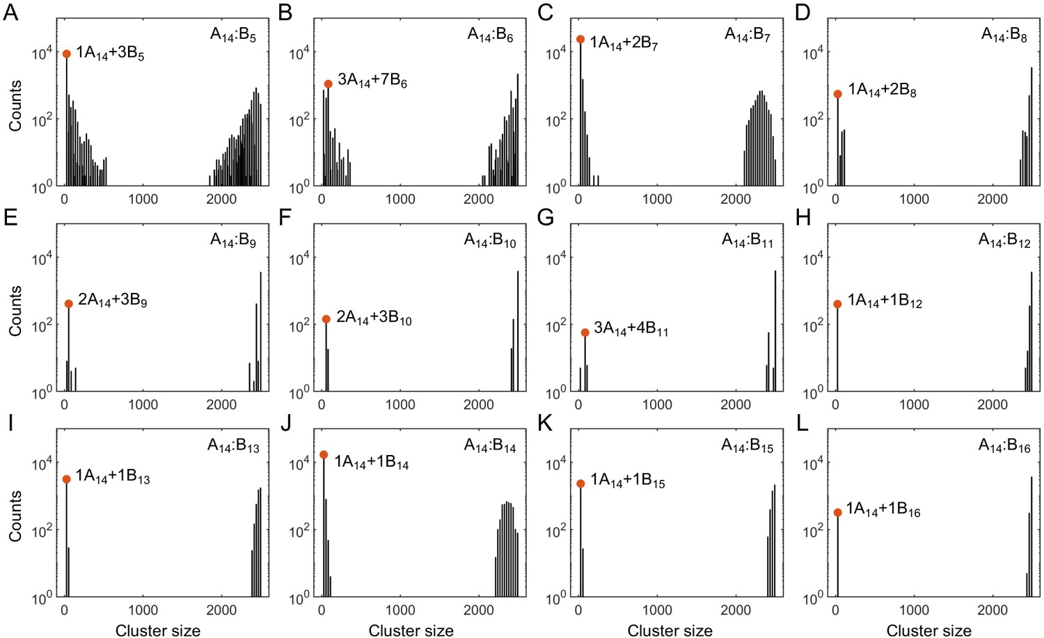
Histograms of cluster size in stickers in (**A–L**) A₁₄:B_5-16 systems at equal global sticker stoichiometry.

Parameters: specific binding strength $U_{0} = 14 k_{B} T$ and total global sticker concentration 6.64 mM. Red dots indicate the dominant oligomer in the dilute phase.

Appendix 1—figure 3

Download asset Open asset

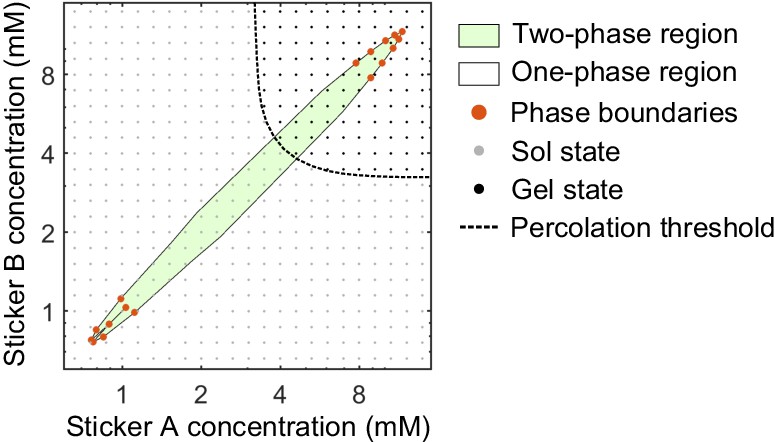
Phase diagram and percolation threshold of A₈:B₈ system.

Phase boundaries (red dots) are measured from MD simulations at $U_{0} = 14 k_{B} T$ . The complete two-phase region (green) and one-phase region (white) are extrapolated based on the phase boundaries from simulations. Sol- (gray dots) and gel- (black dots) states from simulations at $U_{0} = 8 k_{B} T$ where the system remains homogeneous are identified based on the gelation criterions. Percolation threshold (dashed line) is interpolated from the labeled sol- and gel-states.

Appendix 1—figure 4

Download asset Open asset

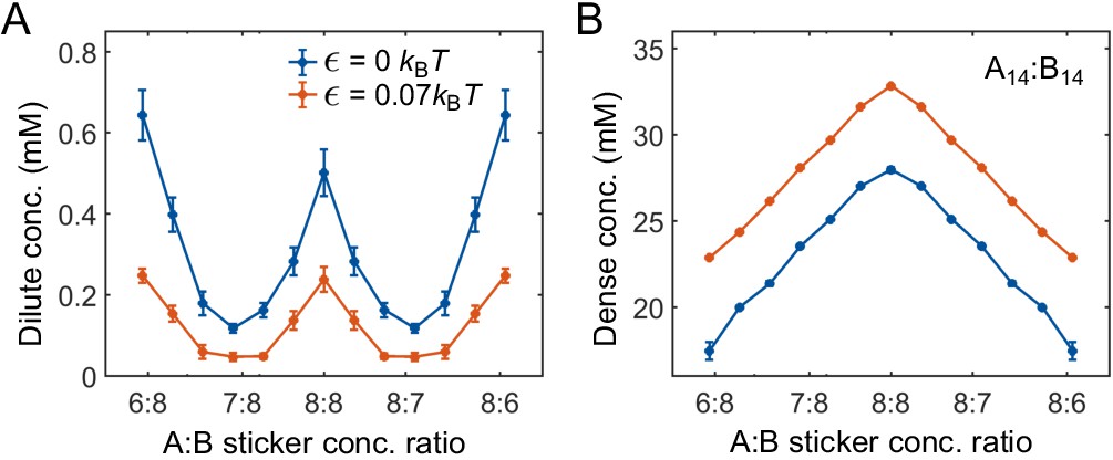
Strength of nonspecific attractive interactions strongly influences simulated dilute-phase boundary.

Total sticker concentrations in (A) dilute and (B) dense phases for A₁₄:B₁₄ system at different global sticker stoichiometries with the additional attractive interaction strength $ϵ = 0 k_{B} T$ (blue) and $ϵ = 0.07 k_{B} T$ (red) ( $σ = 3.5 n m$ and $r_{c} = 5 n m$ in Equation (32)). Parameters: specific interaction strength $U_{0} = 14 k_{B} T$ , total global sticker concentration 6.64 mM.

Appendix 1—figure 5

Download asset Open asset

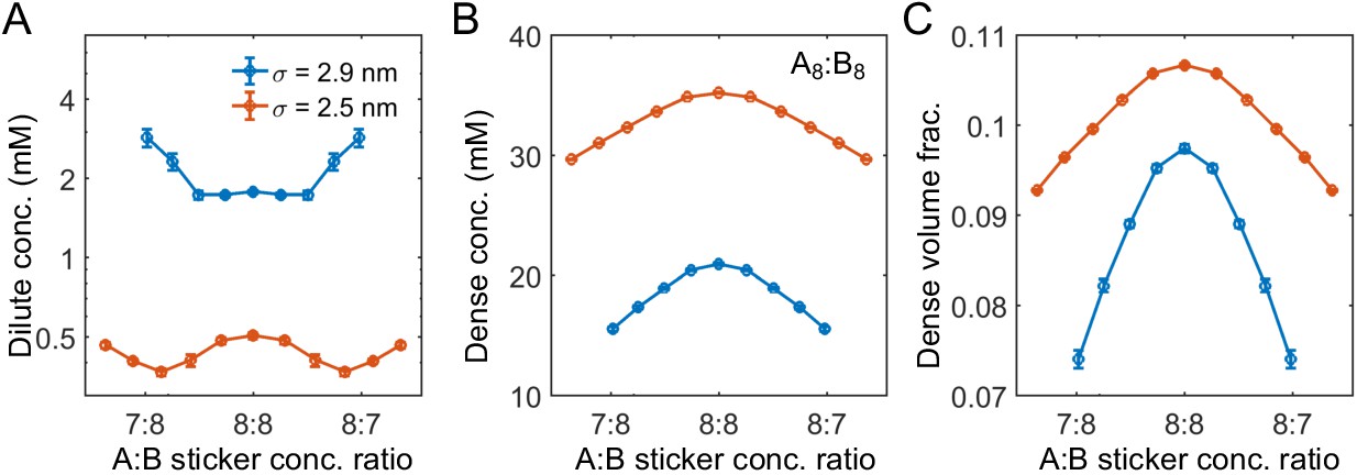
Range of nonspecific repulsive interactions strongly influences phase boundaries in simulations.

Sticker concentrations in (A) dilute and (B) dense phases and (C) volume fraction of polymers in dense phase for A₈:B₈ system at different global sticker stoichiometries with standard repulsive Lennard-Jones potential (Equation (33)) σ = 2.9 nm (blue) and σ = 2.5 nm (red). Parameters: repulsive interaction strength $ϵ = 1 k_{B} T$ , specific interaction strength $U_{0} = 12 k_{B} T$ with cut-off distance r₀ = 1.5 nm, and total global sticker concentration is 6.64 mM. Note that the overlapping volume between two bound stickers is counted once in the volume fraction calculation, that is, two perfectly overlapping stickers only occupy a volume of one sticker.

Appendix 1—figure 6

Download asset Open asset

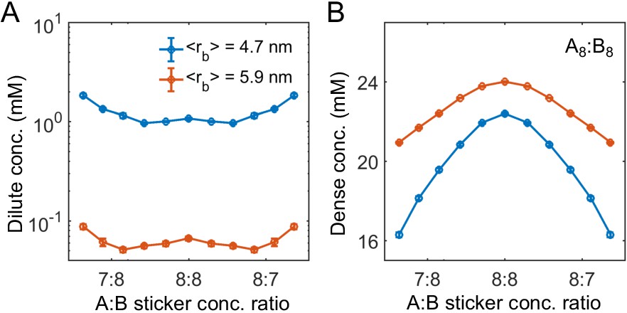
Linker length strongly influences phase boundaries in simulations.

Sticker concentrations in (A) dilute and (B) dense phases for A₈:B₈ system at different global sticker stoichiometries with linkers modeled by a FENE potential (Equation (34)) with $K = 0.3 k_{B} T$ and R₀ = 7 nm (mean linker length 4.7 nm, blue) and $K = 0.15 k_{B} T$ and R₀ = 14 nm (mean linker length 5.9 nm, red). Parameters: repulsive interaction strength $ϵ = 1 k_{B} T$ and length scale σ = 3 nm, specific interaction strength $U_{0} = 12 k_{B} T$ with cut-off distance r₀ = 1.5 nm, and total global sticker concentration 6.64 mM.

Appendix 2—figure 1

Download asset Open asset

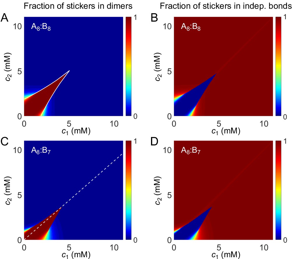
Fraction of stickers in dimers (A) and in independent bonds (B) for A₈:B₈ system.

White curve in (A) is the transition boundary between dimer- and independent bonds-dominated regions predicted by $c_{+} (s)$ and $c_{-} (s)$ . Fraction of stickers in dimers (C) and in independent bonds (D) for A₈:B₇ system. Dashed white line denotes equal polymer stoichiometry.

Appendix 2—figure 2

Download asset Open asset

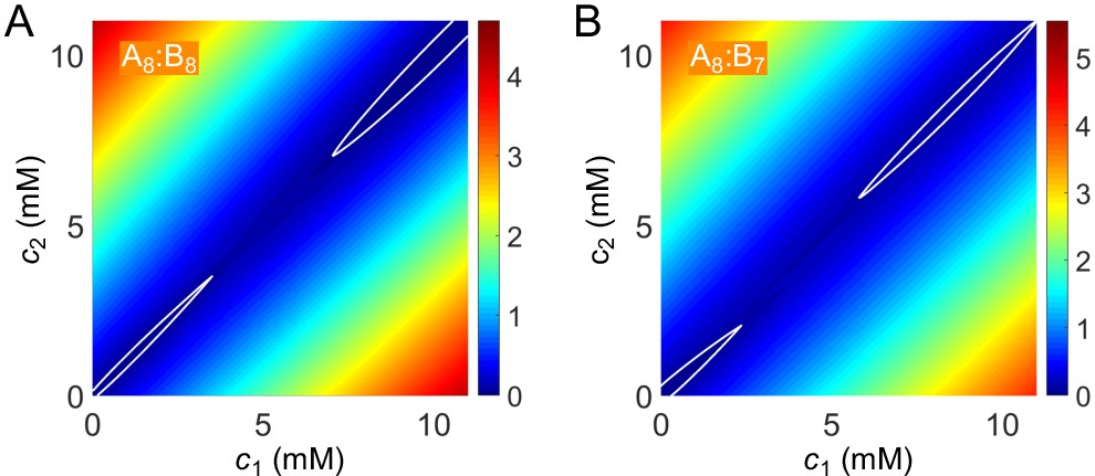
Free-energy density as a function of global sticker concentrations $(c_{1}, c_{2})$ for (A) A₈:B₈ and (B) A₈:B₇ systems.

White curves highlight the basins in the dilute dimer-dominated and dense gel-dominated regions.

Appendix 2—figure 3

Download asset Open asset

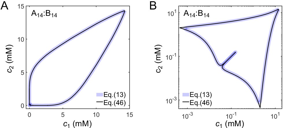
Comparison of phase diagrams derived from the full expression for F (Equation (13)) and the approximate expression (Equation (46)) shown on a (A) linear and (B) log scale for A₁₄:B₁₄ system.

Appendix 2—figure 4

Download asset Open asset

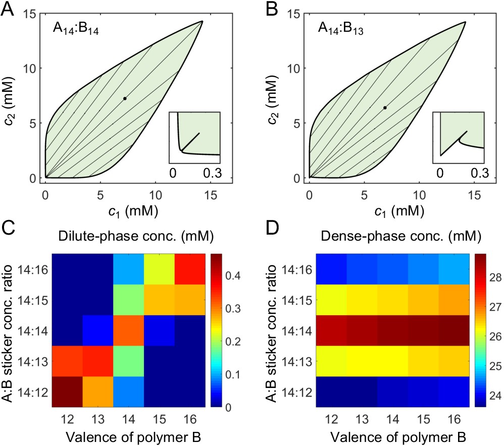
A dimer-gel theory predicts the magic-ratio effect.

Phase diagrams of (A) A₁₄:B₁₄ and (B) A₁₄:B₁₃ systems: one-phase region white, two-phase region green. The dilute- and dense-phase concentrations are connected by representative tie lines. The tie line along the direction of equal polymer stoichiometry is denoted with a black dot. Inset: enlarged dilute-phase boundaries. Sticker concentrations in (C) dilute and (D) dense phases for systems A₁₄:B_12-16 at global sticker stoichiometries 14:12-16 and total sticker concentration 6.64 mM. Parameters: $v_{b} = 7 \times 10^{- 2} {mM}^{- 1}$ , $w_{b} = 5 \times 10^{- 3} {mM}^{- 2}$ , $K_{b} = 3.8 \times 10^{- 3} mM$ , and $K_{d}$ in Appendix 1—table 3.

Appendix 2—figure 5

Download asset Open asset

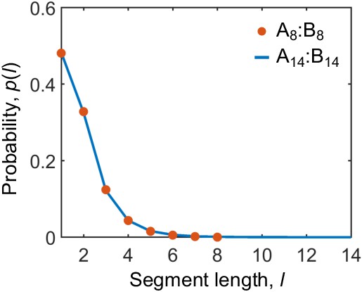
Binding between stickers of different types in the dense phase is correlated.

Probability distribution $p (l)$ for finding a bound sticker to be in a consecutively bound segment of length l in the dense phase of A₈:B₈ and A₁₄:B₁₄ systems at equal stoichiometry.

Appendix 2—figure 6

Download asset Open asset

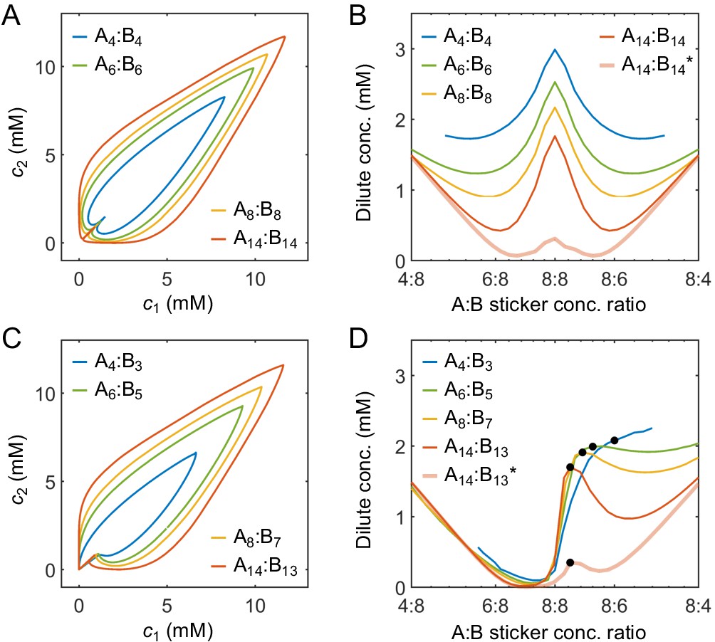
Effects of model parameters on the phase boundaries in the strong-binding regime.

(A) Phase diagrams and (B) dilute-phase concentrations at different global stoichiometries for A₄:B₄ to A₁₄:B₁₄ systems. (C) Phase diagrams and (D) dilute-phase concentrations at different global stoichiometries for A₄:B₃ to A₁₄:B₁₃ systems. Black dots indicate equal *polymer* stoichiometries. Parameters: $K_{b} = 3.8 \times 10^{- 3} mM$ , values of $K_{d}$ in Appendix 1—table 3 for binding strength $U_{0} = 14 k_{B} T$ , $v_{b} = 9 \times 10^{- 2} {mM}^{- 1}$ and $w_{b} = 7 \times 10^{- 3} {mM}^{- 2}$ for all systems except for A₁₄:B_14* and A₁₄:B_13* where $v_{b} = 7 \times 10^{- 2} {mM}^{- 1}$ and $w_{b} = 5 \times 10^{- 3} {mM}^{- 2}$ . Total global sticker concentration 6.64 mM.

Appendix 2—figure 7

Download asset Open asset

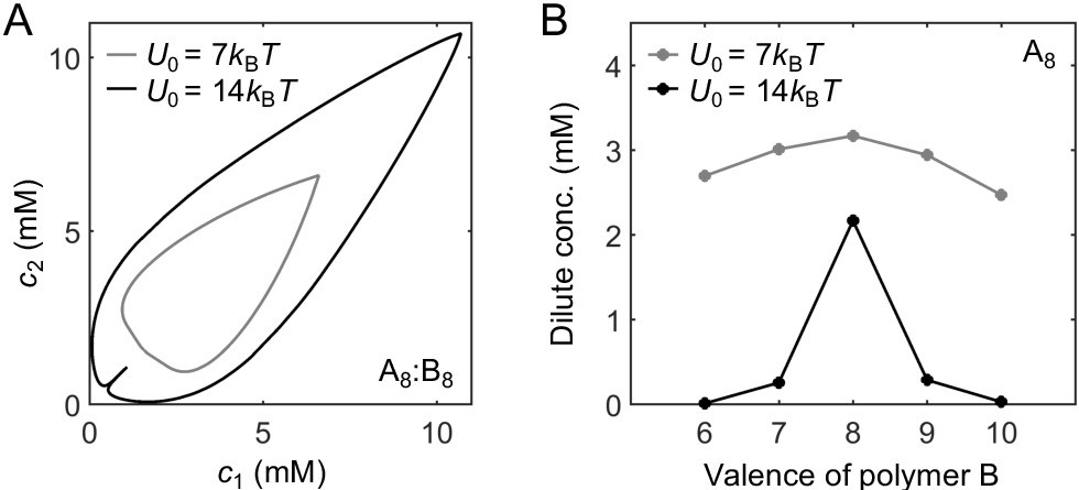
The magic-ratio effect disappears in the weak-binding regime.

(A) Phase diagrams for A₈:B₈ system with different binding strengths $U_{0} = 7 k_{B} T$ (gray) and $U_{0} = 14 k_{B} T$ (black). (B) Dilute-phase concentrations for A₈:B_6-10 systems at equal global sticker stoichiometry with different binding strengths $U_{0} = 7 k_{B} T$ (gray) and $U_{0} = 14 k_{B} T$ (black). Parameters: $K_{b} = 1.88 m M$ for $U_{0} = 7 k_{B} T$ , $K_{b} = 3.8 \times 10^{- 3} mM$ for $U_{0} = 14 k_{B} T$ , values of $K_{d}$ in Appendix 1—table 3, $v_{b} = 9 \times 10^{- 2} {mM}^{- 1}$ , and $w_{b} = 7 \times 10^{- 3} {mM}^{- 2}$ . Total global sticker concentration 6.64 mM.

Author response image 1

Download asset Open asset

Author response image 2

Download asset Open asset

Author response image 3

Download asset Open asset

Author response image 4

Download asset Open asset

Author response image 5

Download asset Open asset

Author response image 6

Download asset Open asset

Tables

Appendix 1—table 1

List of all dilute-phase components and sticker percentages for A₁₄:B₁₄ system at global sticker stoichiometry 1.21.

Comp	1A₁₄	1A₁₄+1B₁₄	2A₁₄+1B₁₄	2A₁₄+2B₁₄	3A₁₄+2B₁₄	4A₁₄+3B₁₄	5A₁₄+3B₁₄
frac	0.10%	37.0%	7.67%	0.38%	19.1%	16.6%	0.38%
comp	5A₁₄+4B₁₄	6A₁₄+4B₁₄	6A₁₄+5B₁₄	7A₁₄+5B₁₄	8A₁₄+6B₁₄	10A₁₄+7B₁₄	17A₁₄+13B₁₄
frac	10.8%	0.85%	0.42%	0.80%	3.45%	0.48%	1.99%

Appendix 1—table 2

Comparison of dilute- and dense-phase concentrations for systems with different total numbers of particles.

Valence (Stoichiometry)	A₁₄:B₁₄ (14:14)	A₁₄:B₁₃ (14:14)	A₁₄:B₁₃ (14:13)
c_dil (mM) for $N = 2500$	0.50 ± 0.06	0.08 ± 0.02	0.39 ± 0.02
c_dil (mM) for $N = 5000$	0.45 ± 0.03	0.12 ± 0.02	0.34 ± 0.03
c_dil (mM) for $N = 2500$	28.0 ± 0.2	27.76 ± 0.09	25.80 ± 0.08
c_den (mM) for $N = 5000$	27.93±0.05	27.82±0.06	25.82±0.06

Appendix 1—table 3

List of dissociation constants from simulations.

	A₁:B₁ (t)	A₁:B₁ (d)	A₁:B₁ (r)	A₂:B₂ (d)	A₂:B₂ (r)
$K_{d} (U_{0} = 0 k_{B} T) (m M)$	49.6	*	48.9	*	12.4
$K_{d} (U_{0} = 7 k_{B} T) (m M)$	1.88	*	1.90	*	0.31
$K_{d} (U_{0} = 14 k_{B} T) (m M)$	5.7e-3	5.9e-3	5.8e-3	7.7e-6	7.1e-6
	A₄:B₃(r)	A₄:B₄ (r)	A₆:B₅ (r)	A₆:B₆ (r)
$K_{d} (U_{0} = 0 k_{B} T) (m M)$	4.32	3.29	1.81	1.52
$K_{d} (U_{0} = 7 k_{B} T) (m M)$	4.5e-2	2.2e-2	4.3e-3	2.2e-3
$K_{d} (U_{0} = 14 k_{B} T) (m M)$	3.77e-9	1.38e-11	6.95e-15	3.00e-17
	A₈:B₆ (r)	A₈:B₇ (r)	A₈:B₈ (r)	A₈:B₉ (r)	A₈:B₁₀ (r)
$K_{d} (U_{0} = 0 k_{B} T) (m M)$	1.15	1.01	0.90	0.79	0.73
$K_{d} (U_{0} = 7 k_{B} T) (m M)$	9.0e-4	4.5e-4	2.5e-4	1.5e-4	1.0e-4
$K_{d} (U_{0} = 14 k_{B} T) (m M)$	4.22e-18	1.26e-20	7.07e-23	1.77e-23	7.59e-24
	A₁₄:B₁₂ (r)	A₁₄:B₁₃ (r)	A₁₄:B₁₄ (r)	A₁₄:B₁₅ (r)	A₁₄:B₁₆ (r)
$K_{d} (U_{0} = 0 k_{B} T) (m M)$	0.37	0.32	0.30	0.32	0.27
$K_{d} (U_{0} = 7 k_{B} T) (m M)$	1.4e-6	6.7e-7	3.8e-7	2.6e-7	1.5e-7
$K_{d} (U_{0} = 14 k_{B} T) (m M)$	2.74e-35	1.08e-37	8.85e-40	1.80e-40	5.16e-41

*footnotetext: $^{(t)}$ theoretical value, $^{({d})}$ direct simulation, and $^{(r)}$ reweighting method.

Additional files

Transparent reporting form: https://cdn.elifesciences.org/articles/62403/elife-62403-transrepform-v1.docx
Download elife-62403-transrepform-v1.docx

Download links

A two-part list of links to download the article, or parts of the article, in various formats.

Downloads (link to download the article as PDF)

Article PDF

Open citations (links to open the citations from this article in various online reference manager services)

Mendeley

Cite this article (links to download the citations from this article in formats compatible with various reference manager tools)

Yaojun Zhang
Bin Xu
Benjamin G Weiner
Yigal Meir
Ned S Wingreen

(2021)

Decoding the physical principles of two-component biomolecular phase separation

eLife 10:e62403.

https://doi.org/10.7554/eLife.62403

Figures

Phase behavior of sticker and spacer associative polymers.

Coarse-grained molecular-dynamics simulations of two-component multivalent associative polymers.

Simulations of associative polymers reveal a magic-number effect with respect to relative valence.

Simulations of associative polymers reveal a magic-ratio effect with respect to polymer stoichiometry.

Simulations of associative polymers reveal a magic-ratio effect.

A dimer-gel theory predicts the magic-ratio effect.

Coarse-grained molecular-dynamics simulations of two-component multivalent associative polymers.

Histograms of cluster size in stickers in (A–L) A₁₄:B_5-16 systems at equal global sticker stoichiometry.

Phase diagram and percolation threshold of A₈:B₈ system.

Strength of nonspecific attractive interactions strongly influences simulated dilute-phase boundary.

Range of nonspecific repulsive interactions strongly influences phase boundaries in simulations.

Linker length strongly influences phase boundaries in simulations.

Fraction of stickers in dimers (A) and in independent bonds (B) for A₈:B₈ system.

Free-energy density as a function of global sticker concentrations $(c_{1}, c_{2})$ for (A) A₈:B₈ and (B) A₈:B₇ systems.

Comparison of phase diagrams derived from the full expression for F (Equation (13)) and the approximate expression (Equation (46)) shown on a (A) linear and (B) log scale for A₁₄:B₁₄ system.

A dimer-gel theory predicts the magic-ratio effect.

Binding between stickers of different types in the dense phase is correlated.

Effects of model parameters on the phase boundaries in the strong-binding regime.

The magic-ratio effect disappears in the weak-binding regime.

Tables

List of all dilute-phase components and sticker percentages for A₁₄:B₁₄ system at global sticker stoichiometry 1.21.

Comparison of dilute- and dense-phase concentrations for systems with different total numbers of particles.

List of dissociation constants from simulations.

Additional files

Transparent reporting form

Download links

Downloads (link to download the article as PDF)

Open citations (links to open the citations from this article in various online reference manager services)

Cite this article (links to download the citations from this article in formats compatible with various reference manager tools)

Be the first to read new articles from eLife

Share this article

Cite this article

Phase behavior of sticker and spacer associative polymers.

Coarse-grained molecular-dynamics simulations of two-component multivalent associative polymers.

Simulations of associative polymers reveal a magic-number effect with respect to relative valence.

Simulations of associative polymers reveal a magic-ratio effect with respect to polymer stoichiometry.

Simulations of associative polymers reveal a magic-ratio effect.

A dimer-gel theory predicts the magic-ratio effect.

Coarse-grained molecular-dynamics simulations of two-component multivalent associative polymers.

Histograms of cluster size in stickers in (A–L) A14:B5-16 systems at equal global sticker stoichiometry.

Phase diagram and percolation threshold of A8:B8 system.

Strength of nonspecific attractive interactions strongly influences simulated dilute-phase boundary.

Range of nonspecific repulsive interactions strongly influences phase boundaries in simulations.

Linker length strongly influences phase boundaries in simulations.

Fraction of stickers in dimers (A) and in independent bonds (B) for A8:B8 system.

Free-energy density as a function of global sticker concentrations (c1,c2) for (A) A8:B8 and (B) A8:B7 systems.

Comparison of phase diagrams derived from the full expression for F (Equation (13)) and the approximate expression (Equation (46)) shown on a (A) linear and (B) log scale for A14:B14 system.

A dimer-gel theory predicts the magic-ratio effect.

Binding between stickers of different types in the dense phase is correlated.

Effects of model parameters on the phase boundaries in the strong-binding regime.

The magic-ratio effect disappears in the weak-binding regime.

List of all dilute-phase components and sticker percentages for A14:B14 system at global sticker stoichiometry 1.21.

Comparison of dilute- and dense-phase concentrations for systems with different total numbers of particles.

List of dissociation constants from simulations.

Transparent reporting form

Downloads (link to download the article as PDF)

Open citations (links to open the citations from this article in various online reference manager services)

Cite this article (links to download the citations from this article in formats compatible with various reference manager tools)

Histograms of cluster size in stickers in (A–L) A₁₄:B_5-16 systems at equal global sticker stoichiometry.

Phase diagram and percolation threshold of A₈:B₈ system.

Fraction of stickers in dimers (A) and in independent bonds (B) for A₈:B₈ system.

Free-energy density as a function of global sticker concentrations $(c_{1}, c_{2})$ for (A) A₈:B₈ and (B) A₈:B₇ systems.

Comparison of phase diagrams derived from the full expression for F (Equation (13)) and the approximate expression (Equation (46)) shown on a (A) linear and (B) log scale for A₁₄:B₁₄ system.

List of all dilute-phase components and sticker percentages for A₁₄:B₁₄ system at global sticker stoichiometry 1.21.