Synthesis of a comprehensive population code for contextual features in the awake sensory cortex
- Biophysics Graduate Group, United States
- Department of Molecular and Cell Biology, United States
- The Edmond and Lily Safra Center for Brain Sciences and The Life Sciences Institute, The Hebrew University of Jerusalem, Israel
- The Helen Wills Neuroscience Institute, University of California, Berkeley, United States
Figures
Figure 1 with 1 supplement
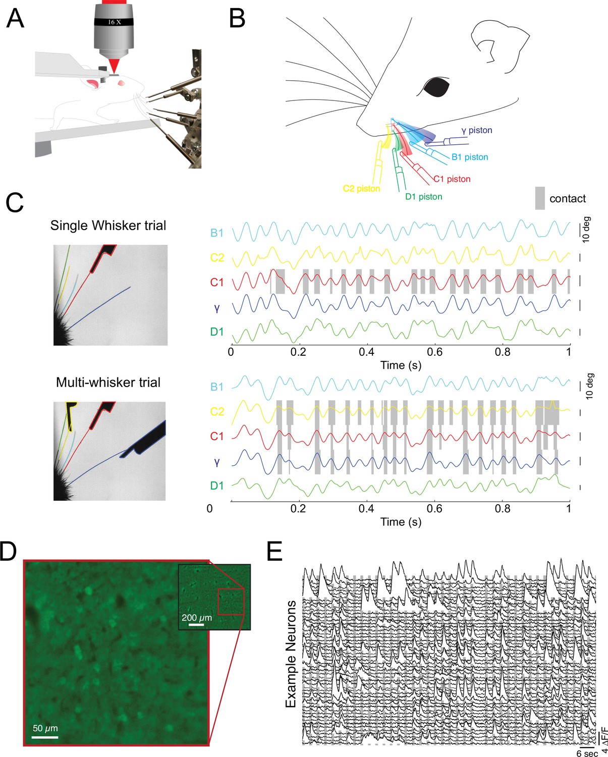
Probing cortical population codes of higher-order features during active touch.
(A) Schematic of the experimental preparation showing a locomoting mouse under a two-photon microscope actively contacting five individual pistons with five individual whiskers (the rest are trimmed just before the experiment, see Materials and methods). (B) Schematic of the multi-whisker stimulator. (C) Top left: single frame of a high-speed video where only the C1 whisker was presented with a piston. Top right: angle traces for each of the five whiskers. Touch events between the C1 whisker and the C1 piston are shaded in gray. Bottom: same as above but for a trial where the C2, C1, and γ pistons were presented. (D) Example field of view from a single depth (pixel values are the variance across time). (E) Two minutes of consecutive fluorescence measurements from 50 randomly chosen neurons in a single example experiment. Vertical gray bars indicate the presentation of different multi-piston stimuli.
Figure 1—figure supplement 1
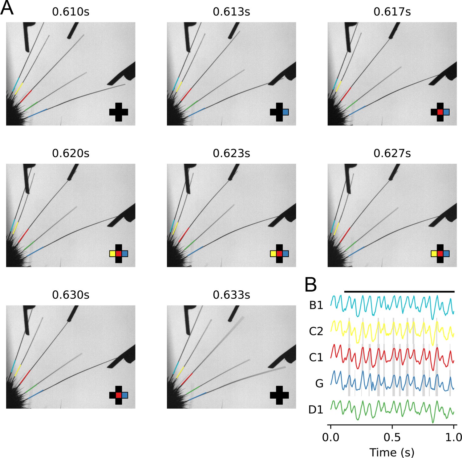
Whisker tracking during an example trial.
(A) Frames from a high-speed video of the whiskers whisking during a single trial. By properly trimming the whiskers and positioning the pistons, each whisker can only come into contact with a single piston, and can only contact that piston when it’s presented. In this trial, the C1, C2, and Gamma pistons were presented. The whiskers are traced offline (see Materials and methods). The 10% of each trace closest to the mouse’s face is overlaid and used to compute each whisker’s angle. The crosshair in the bottom right corner shows when the tip of the whisker’s trace (not shown) overlaps with its respective piston’s region of interest (ROI) (not shown) and is defined as touching that piston. (B) Plots of each whisker’s measured angle during the example trial in (A). Touch events are overlaid in gray and the duration of the stimulus’s presentation is shown at the top (see Materials and methods for touch identification analysis).
Figure 2 with 4 supplements
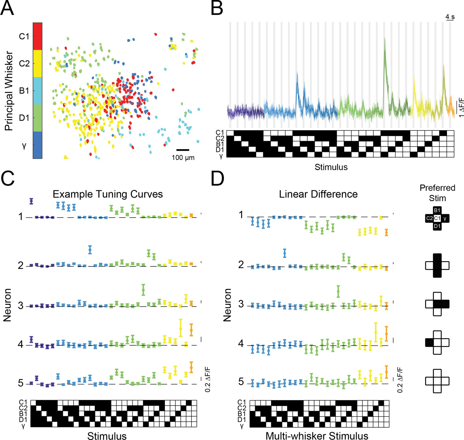
Diverse and selective representations of higher-order tactile stimuli in mouse barrel cortex.
(A) Example map of principal whisker preference in L2/3 of one mouse. (B) Top: calcium responses from an example neuron to each of the 31 possible combinations of the five pistons (mean and 95% confidence intervals [C.I.]). Traces are colored-coded by the number of whiskers contacting pistons in each stimulus (1–5 whiskers). Vertical gray bars indicate presence of the tactile stimulus. Bottom: diagram of the 31 corresponding piston combination stimuli. White squares indicate the presence of the corresponding piston and black indicates the absence. (C) Example tuning curves for five neurons in L2/3 of S1 for all 31 stimuli and colored as in (B). Neuron three corresponds to the neuron shown in panel (B). (D) Left: the computed difference of the observed response to each multi-whisker stimulus from the linear sum of the component responses when each whisker contacts its corresponding piston alone for the five example neurons in (C), or ‘Linear Difference’. All error bars are bootstrapped 95% CI. Right: diagram of each neuron’s preferred stimulus.
Figure 2—figure supplement 1
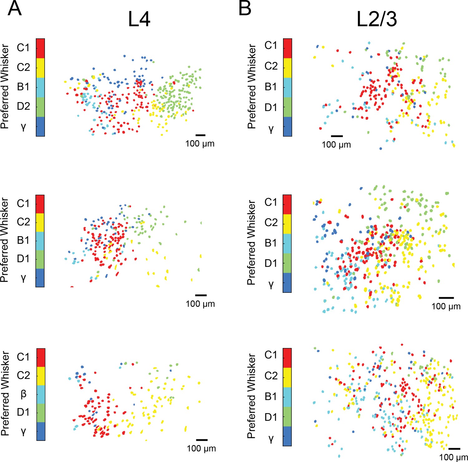
Maps of single whisker tuning in awake, whisking mice.
(A) Three maps of principal whisker preference for L4 neurons from three Scnn1-Cre mice injected with AAV-syn-flexed-GCaMP6s. (B). Same as a but for three mice recorded in L2/3 using Camk2-tTa;tetO-GCaMP6s mice.
Figure 2—figure supplement 2
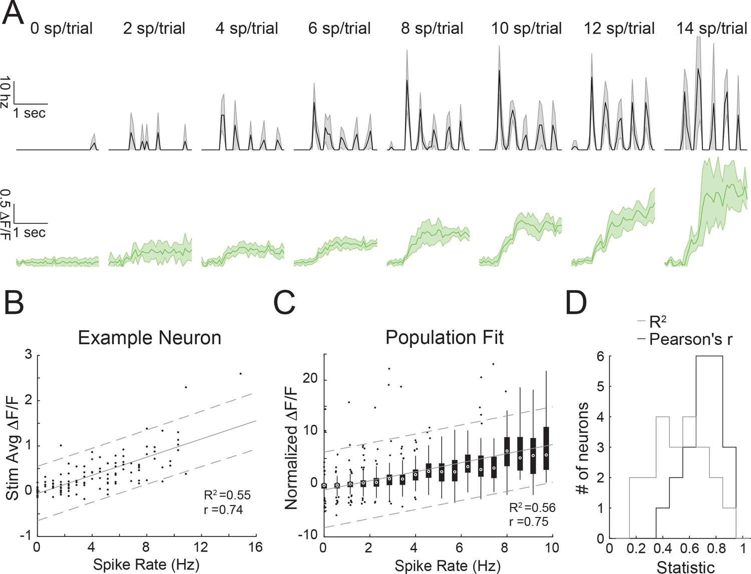
The transform from spiking to fluorescence in GCaMP6s-expressing neurons in Camk2-tTa;tetO-GCaMP6s mice.
(A) Top: trial-averaged instantaneous spike rate of a neuron for trials that contain specific numbers of spikes (mean with s.e.m.). The neuron is recorded in vivo via two-photon targeted loose patch during visual stimulation with oriented gratings. Bottom: Trial-averaged calcium responses of the same trials above (mean with s.e.m.). (B) Average dF/F versus spike rate per trial for the same example neuron. Gray lines indicate a linear regression with 95% confidence intervals (C as in B) but for a population of recorded cells (n=21). Box plots are shown for all trials that had a specific number of spikes. Gain normalization of each cell’s change in fluorescence was necessary to produce a good population fit. (D) Histograms of the coefficient of determination (gray) and Pearson’s correlation (black) for all analyzed neurons.
Figure 2—figure supplement 3
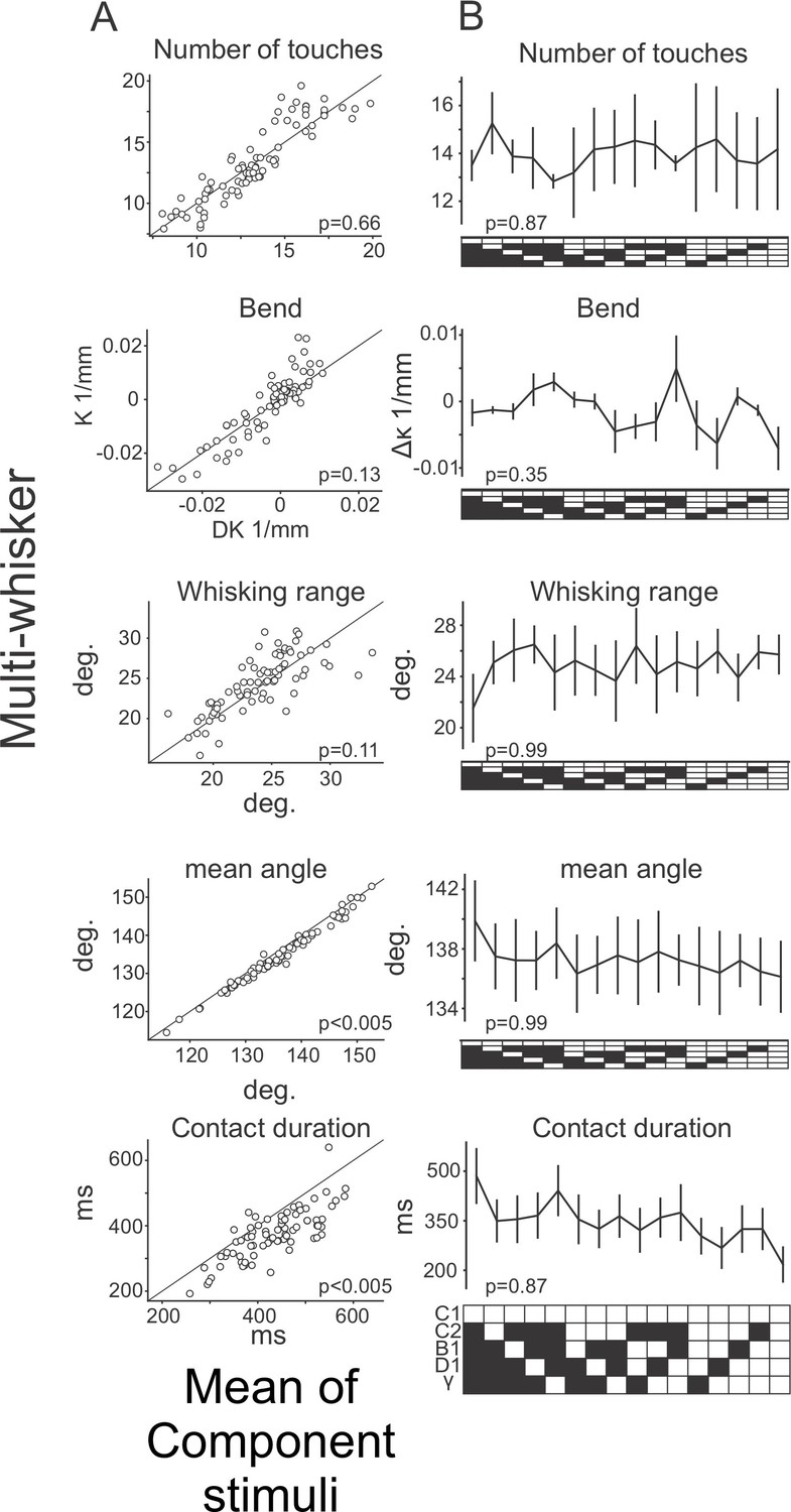
Whisker kinematics across the stimulus set.
(A) Scatter plots comparing the mean of each indicated kinematic variable during multi-whisker stimuli (y-axis) and the mean across the component single whisker stimuli for each corresponding multi-whisker stimulus (x-axis). (B) The mean of each indicated kinematic variable for the C1 whisker was compared across all stimuli that contain the C1 piston. N=3 mice.
Figure 2—figure supplement 4
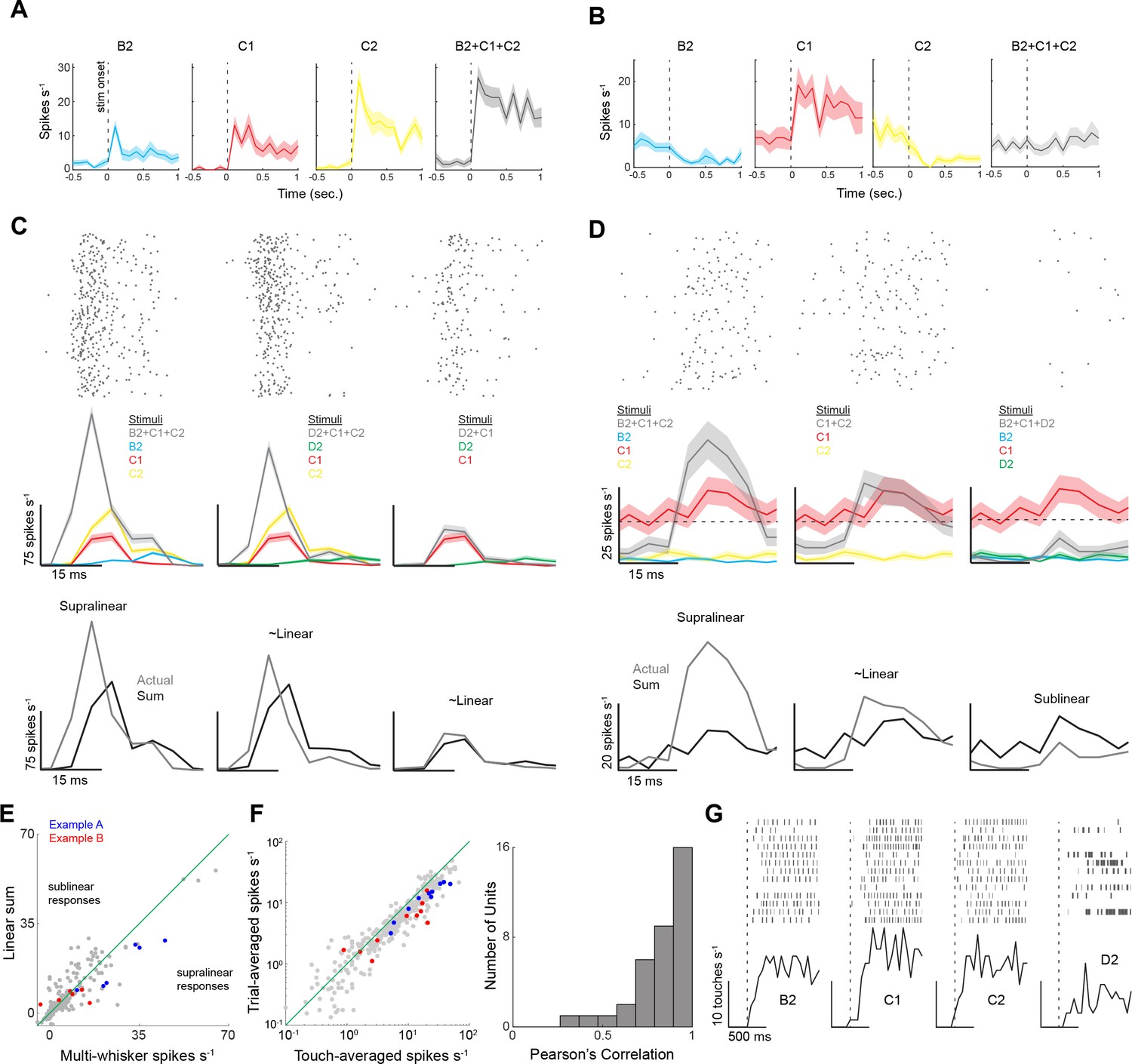
Electrophysiological measurement of supralinear summation during multi-whisker contact.
(A, B) Trial-averaged firing rates (composed of many touches per trial) in two example neurons for three different single whisker stimuli and their multi-whisker combination. Firing rates for the first second of object presentation is shown. (C) Top: example raster plots aligned to the onset (vertical line) of multi-whisker touch. Spiking is aligned to the onset of principal whisker (C2) contact. Data are from the example neuron in panel (A). Middle: Peristimulus time histograms (PSTHs) of contact-triggered spiking for single and multi-whisker touch (color code as in [A]). Bottom: comparison of the actual multi-whisker PSTH to the summed PSTHs of the component single-whisker responses. The baseline spike rate (calculated during free-whisking periods) was subtracted from each PSTH, to avoid summing spontaneous activity. (D) Data from the second example neuron, processed identically as (B). The horizontal dotted line is the neuron’s baseline firing rate, measured during free whisking. Two stimuli (whiskers [B] and [C]) suppress spiking below baseline during repeated touch, hence the apparently different baseline firing rates prior to each touch. (E) Scatter plot comparing multi-whisker touch responses to the linear sum of the single whisker responses. (F) Left: scatter plot comparing the trial-averaged spike rate to the touch-averaged spike rate. The mean trial-averaged spike rate was calculated from the 500 ms period following the onset of stimulus presentation. The mean touch-averaged spike rate was calculated from the 40 ms period following each touch event. The example neurons in panels (A and B) are shown in blue and red dots, respectively. Right: histogram of the Pearson correlation between the touch- and trial-averaged spike rates for each neuron. (G) Histogram of touch rate for the different single whisker stimuli used in this experiment. The dotted vertical line is the onset of stimulus presentation when the piston enters the whisking field.
Figure 3 with 4 supplements
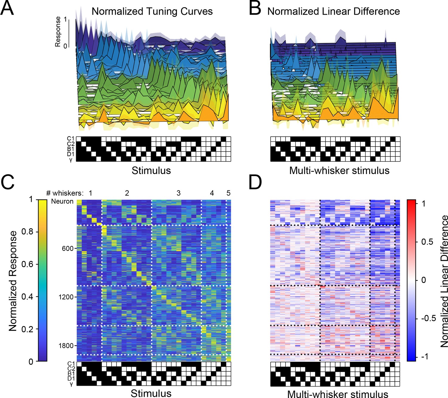
Sparse, high-dimensional population codes of higher-order tactile features generated through stimulus-specific supra-linear summation.
(A) 31 example tuning curves from one field of view in one mouse showing neurons that exhibit a peak response for each of the 31 presented stimuli. Shaded regions are 95% confidence intervals (B) Linear difference of the 31 neurons in (A). (C) Normalized, cross-validated tuning curves for all sensory-driven neurons in awake, whisking mice. Neurons are ordered along the vertical axis by the stimulus to which they responded best. (D) The normalized linear difference for the neurons in (C).
Figure 3—figure supplement 1
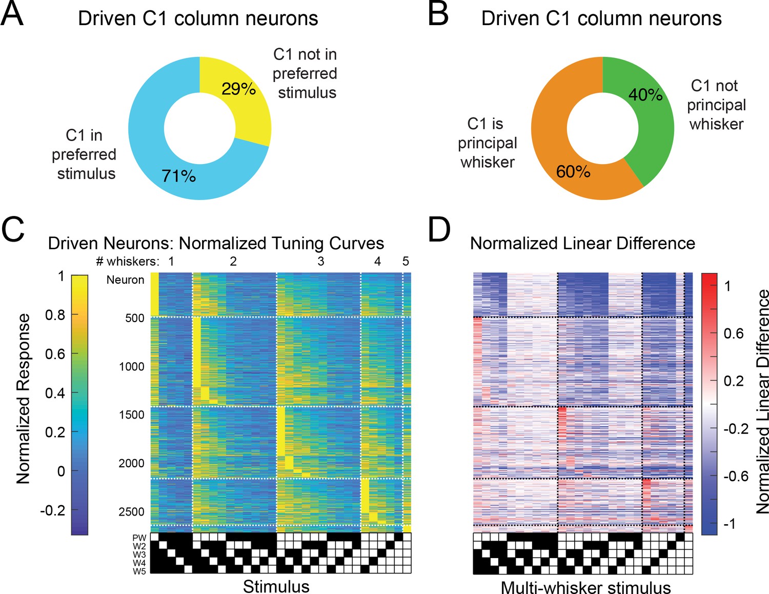
The preferred multi-whisker stimulus for each neuron nearly always includes its principal whisker (PW).
(A) Breakdown of C1 column neurons by whether they have C1 in their best stimulus or not. (B) Breakdown of C1 column neurons by whether C1 is their PW. (C) Normalized tuning curves for all sensory-driven neurons in awake, whisking mice. Neurons are ordered on the vertical axis first by the number of whiskers in their preferred stimulus (1–5), and secondly by their selectivity. The PW is set as the whisker that has the largest weight when fit by a general linear model. The stimuli are ordered by the whisker rank of each neuron’s generalized linear model fit (which is specific to each neuron). Note that the maximal values for each neuron’s tuning curve (rows of the matrix) almost always contains the PW. (D) Normalized linear difference for the neurons in (A) ordered in the same way.
Figure 3—figure supplement 2
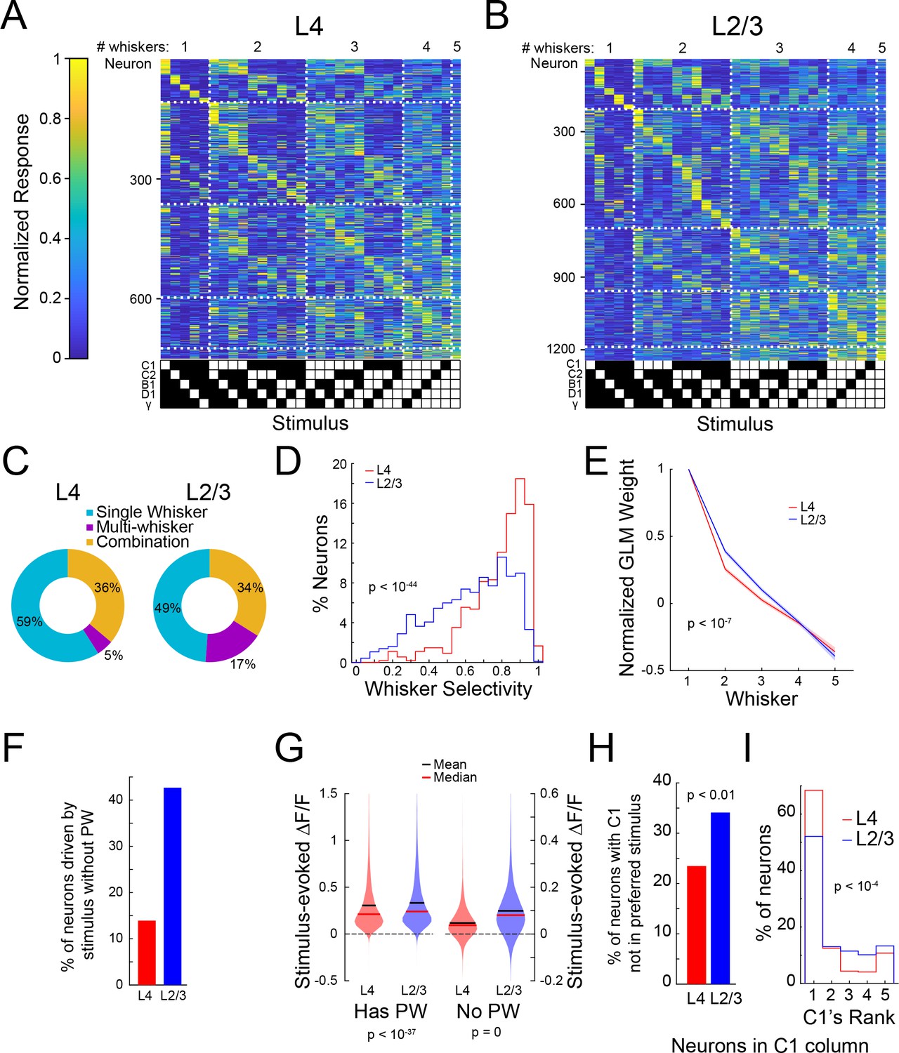
Differences between tactile representations in L4 and L2/3.
(A) Normalized, cross-validated tuning curves for recorded L4 neurons. (B) Same as A but for L2/3 neurons. (C) Ring graphs showing the percentage of driven neurons that were single-whisker responsive, responded to multiple single whisker stimuli, or did not respond to any single whisker stimulus but responded to a multi-whisker stimulus ‘combination’. (D) Histograms comparing the whisker selectivity of L4 and L2/3 neurons that are significantly driven by at least one single-whisker stimulus (p<10–44, Wilcoxon ranksum; L4 n=541, L2/3 n=935). (E) Average of normalized, rank-ordered whisker weights from general linear models fit to each neuron (p<10–7, 2-way analysis of variance [ANOVA]; L4 n=847, L2/3 n=1415). (F) Percentage of neurons that had at least one significant response to a stimulus that did not include the principal whishker (PW). (G) Left: violin plots of the mean responses for all multi-whisker stimulus combinations for all driven neurons containing the PW (p<10–37, Wilcoxon ranksum; L4: n=12705, L2/3: n=21225). Right: same but for stimuli that did not contain the PW (p=0, Wilcoxon ranksum; L4: n=9317, L2/3: n=15565). (H) Percentage of C1 column neurons that did not have C1 in their preferred stimulus (p<0.01, permutation test; L4 n=345, L2/3 n=384). (I) Distribution of C1 column neurons’ rank of the C1 whisker within their generalized linear model-computed whisker weights (p<10–4, Kruskal-Wallis test; L4 n=345, L2/3 n=384).
Figure 3—figure supplement 3
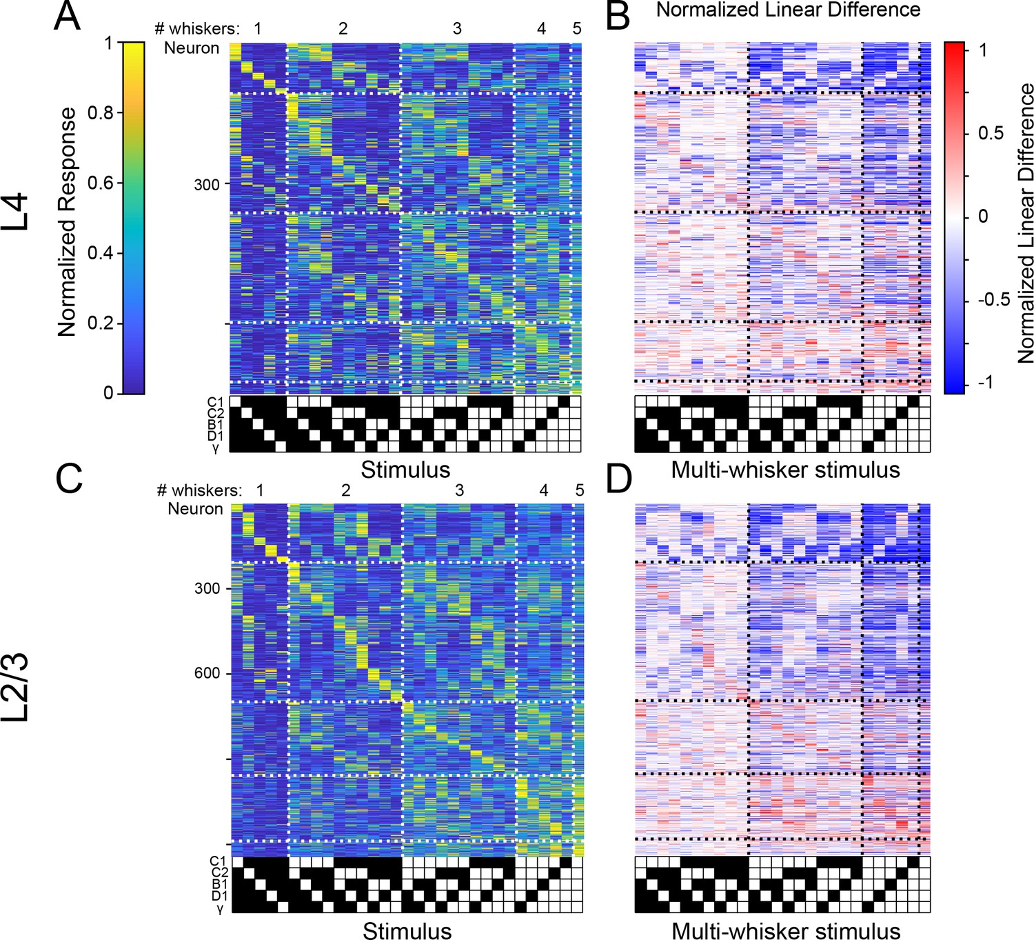
Comparison between L4 and L2/3 of barrel cortex.
(A) Normalized tuning curves of 50% of the data for all sensory-driven L4 neurons from awake mice ordered on tuning curves calculated on the remaining 50% of data. (B) Normalized linear difference for the neurons and data shown in (A). (C) Same as A but for L2/3 neurons recorded in awake mice. (D) Normalized linear difference for the neurons in (C).
Figure 3—figure supplement 4
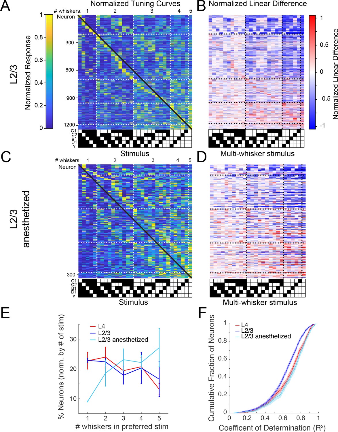
Altered population codes in anesthetized, passively stimulated mice.
(A) Normalized, cross-validated tuning curves for all sensory-driven L2/3 neurons from awake mice. The black diagonal line depicts the expected population diagonal if the neural population uniformly covers the stimulus space. (B) Normalized linear difference for the neurons in (A). (C) Same as A but for L2/3 neurons recorded in anesthetized mice whose whiskers were stimulated with piezoelectric benders. (D) Normalized linear difference for the neurons in (C). (E) Percent of neurons whose preferred stimulus contains 1, 2, 3, 4, or five whiskers, normalized by the number of stimuli presented in each category (mean and 95% confidence intervals; L4 p=0.10, n=3; L2/3 p=0.72, n=3; L2/3 anesthetized p=0.08, n=3; one-way analysis of variance [ANOVA]). (F) Cumulative density functions of the coefficient of determination (R2) from a general linear model fit of tuning curves for L4, L2/3 awake, and L2/3 anesthetized neurons (L2/3 vs. L2/3 anesthetized p<10–17; L4 vs. L2/3 p<10–9; L4 vs. L2/3 anesthetized p=0.03, Wilcoxon ranksum, Bonferroni multiple comparisons correction; L4 n=847, L2/3 n=1415, L2/3 anesthetized n=635).
Figure 4 with 7 supplements
Stimulus-specific supra-linear summation in the primary visual cortex.
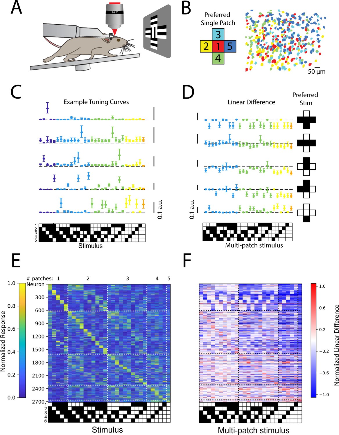
(A) Schematic of the experimental preparation. (B) Example imaged field of view in layer 2/3 where each identified neuron is color coded according to its preferred single stimulus patch. (C) Five example tuning curves from neurons preferring different numbers of patches. Neurons are from four fields of view in layer 2/3 of three mice. Error bars are bootstrapped 95% confidence intervals (D) Linear difference of the five neurons in (C). (E) Normalized, cross-validated tuning curves for all sensory-driven neurons in awake, whisking mice. Neurons are ordered along the vertical axis by the stimulus to which they responded best. N=10 fields of view, 6 animals. (F) The normalized linear difference for the neurons in (E).
Figure 4—figure supplement 1
Comparison between L4 and L2/3 of visual cortex.
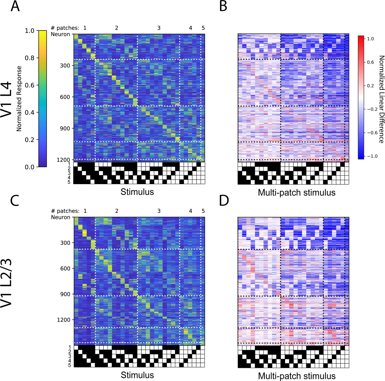
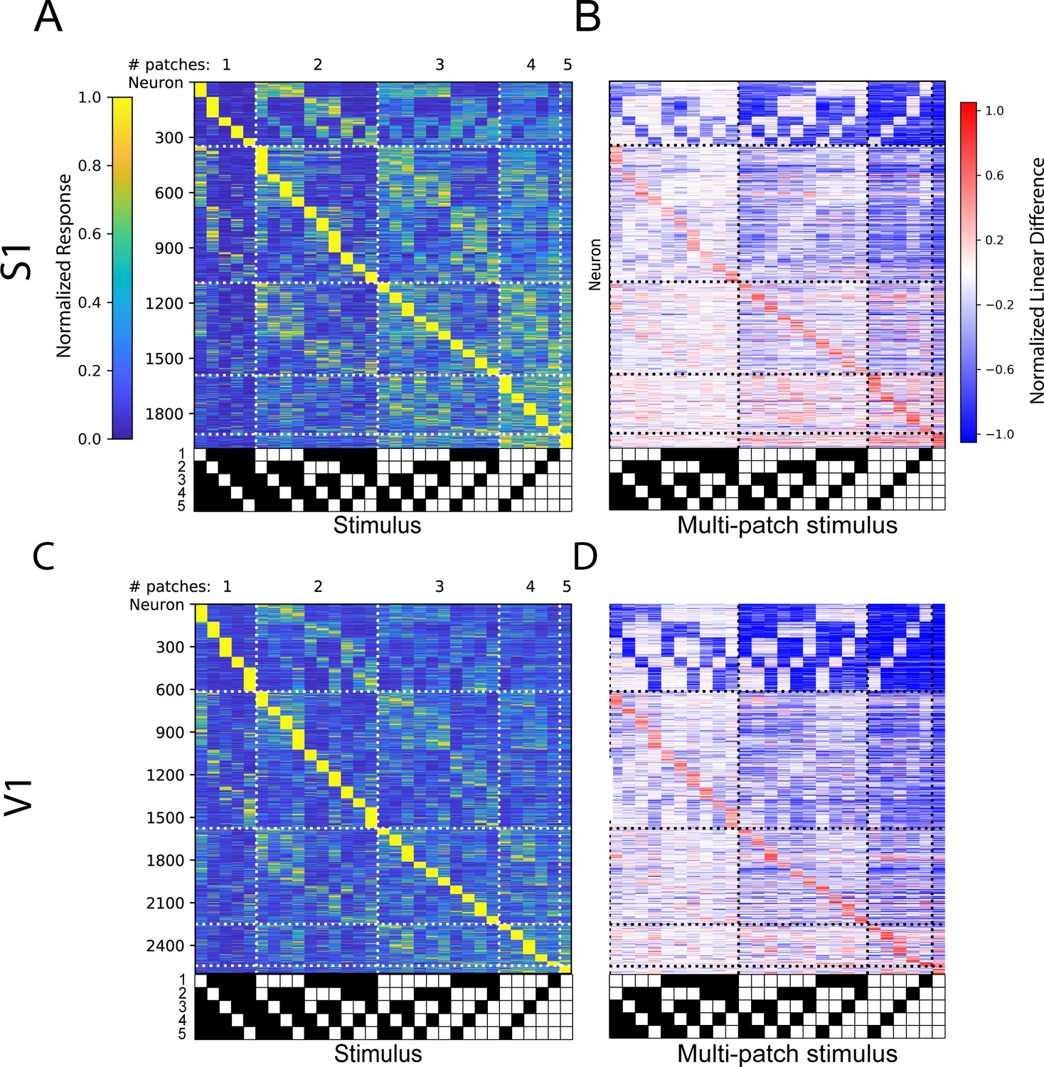
(A) Normalized tuning curves computed from 50% of the data for all sensory-driven V1 L4 neurons from awake mice ordered on tuning curves calculated on the remaining 50% of data. N=5 fields of view (FOVs), 3 animals. (B) Normalized linear difference for the neurons in (A). (C) Same as (A) but for V1 L2/3 neurons recorded in awake mice. N=5 FOVs, 3 animals. (D). Normalized linear difference for the neurons in (C).
Figure 4—figure supplement 2
Analogous population code for 15° grating patches.
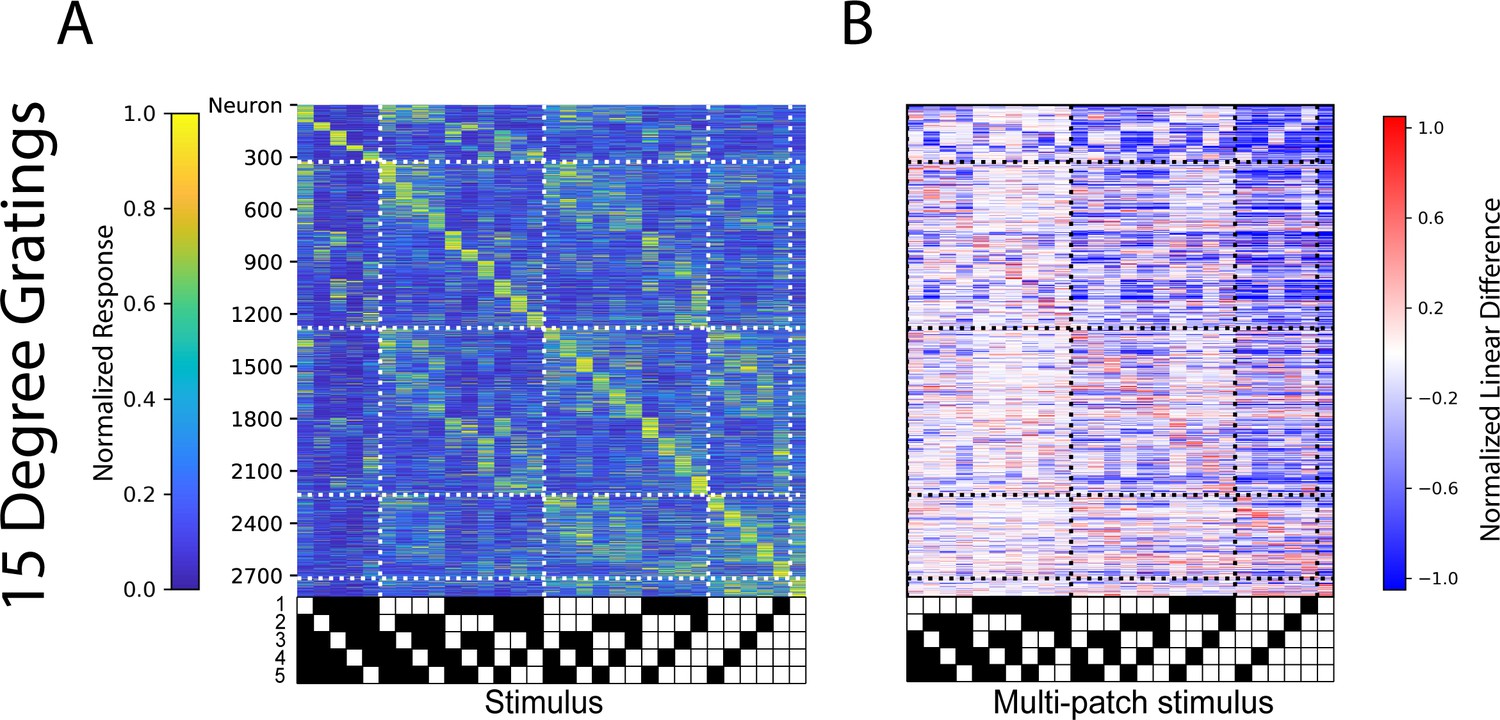
(A) Cross-validated tuning curves and (B) linear difference plots of neurons in layer 4 and layer 2/3 of V1 for 15 visual degree patches (right). N=10 fields of view, 6 animals.
Figure 4—figure supplement 3
Effect of deconvolution on tuning curve calculation.
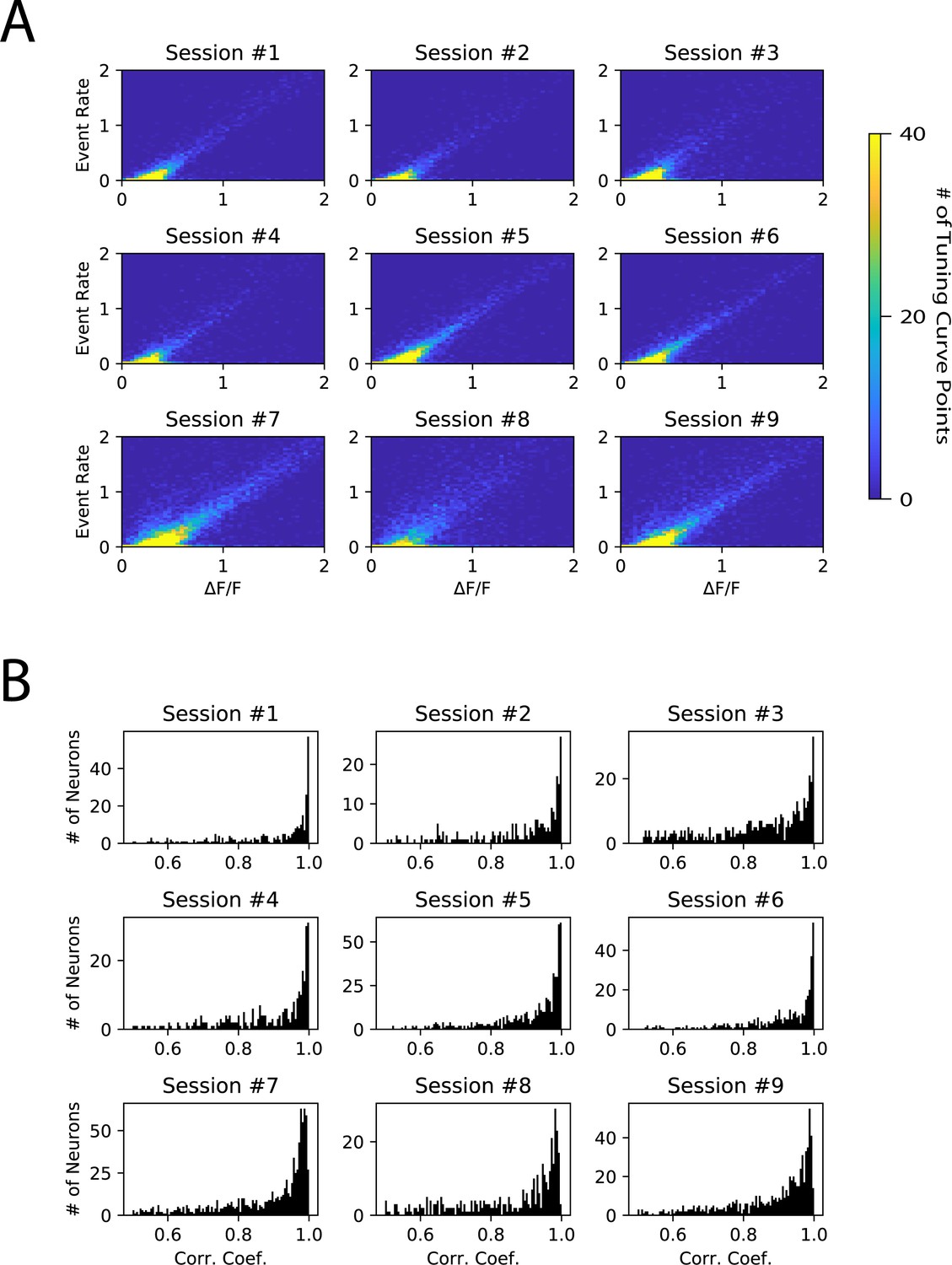
(A) 2-D histogram of tuning curve elements computed using ∆F/F as compared to deconvolved event rate. Each plot is from one imaging session (either S1 L2/3 or S1 L4). Only trials following catch trials were analyzed, to avoid contamination from decaying calcium transients from the previous trial. (B) Histograms of correlation coefficients between tuning curve computed with deconvolved event rate, and tuning curve computed with ∆F/F. 52% of neurons had R>0.9. One plot per S1 imaging session. N=9 fields of view, 6 animals.
Figure 4—figure supplement 4
Non-cross validated tuning curves and linear difference plots of S1 and V1 neurons.
(A) Non-cross validated tuning curves and (B) linear difference plots for S1 layer 4 and layer 2/3 experiments, sorted on and displaying an average of all trials, rather than sorted based on held out trials. (C,D) Same as (A,B), for V1.
Figure 4—figure supplement 5
Alternative cross-validated tuning curves and linear difference plots of S1 and V1 neurons.
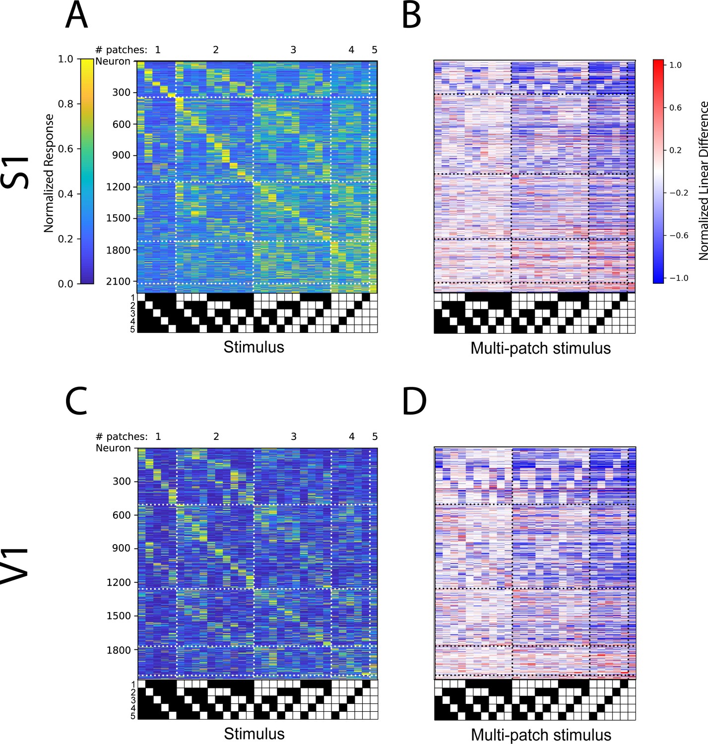
(A) Cross-validated tuning curves and (B) linear difference plots for S1 layer 4 and layer 2/3 experiments, sorted based on two-thirds of trials, and displaying the average response across the final third of trials. Neurons were selected based on correlation coefficient between responses in the first and second third of trials. (C,D) Same as (A,B), for V1.
Figure 4—figure supplement 6
Supra-linear difference plots reflect true deviation from linearity in S1.
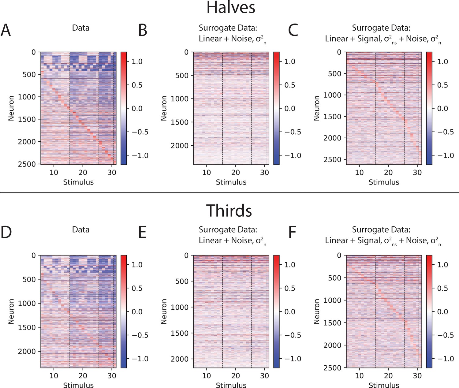
(A) Linear difference plots, computed based on actual data, reproduced from Figure 3D. (B) Linear difference plots, computed based on a surrogate dataset, in which the underlying tuning curve was constructed to reflect a linear sum of single-whisker responses. Stimulus-independent noise was added to each half of the data, such that the total variability across halves of the data was matched with the same quantity for the data linear differences. ‘Reliably estimated’ tuning curves were selected for display in the same way as for the actual data (see Materials and methods). (C) Same as (B), but for a surrogate dataset in which an identical stimulus-dependent signal was added to both halves of the data, such that the total variability across stimuli was matched with the same quantity for the data linear difference, as well as the stimulus-dependent noise in (B). (D–F) Same as (A–C), but operating on, or applying noise to, thirds of the data as in Figure 4—figure supplement 5.
Figure 4—figure supplement 7
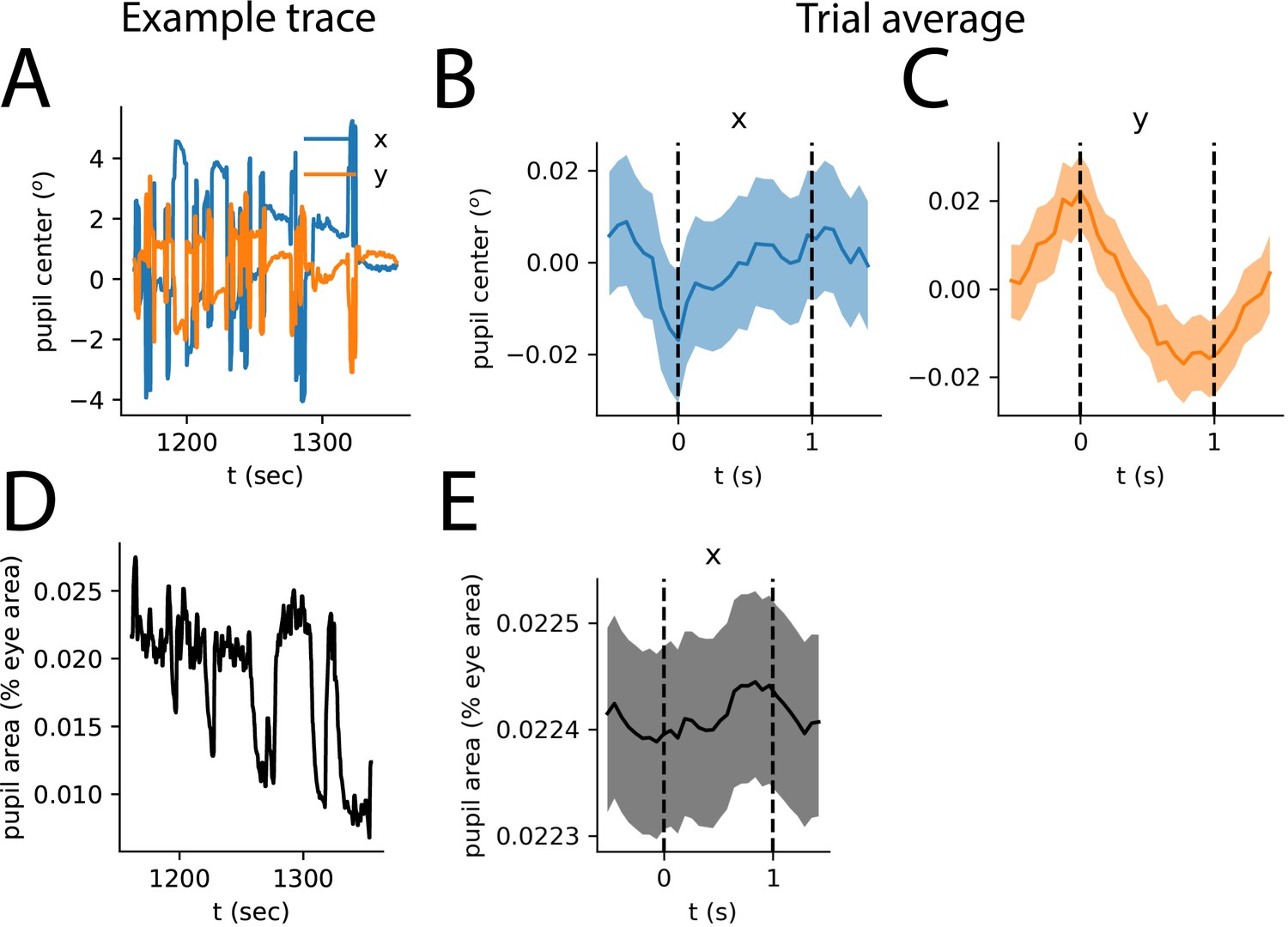
Eye movements are not strongly synchronized to stimulus presentation.
(A) Representative example traces of x and y positions of pupil center, in visual degrees, relative to their means. (B) Trial average of x-position of pupil center. Dashed lines represent onset (0 s) and offset (1 s) of visual stimulus presentation. The shaded area represents bootstrapped 68% confidence interval across trials. (C) Same as (B), for y-position of pupil center. (D) Same as (A), for pupil area over the same time interval. (E) Same as (B,C) for pupil area.
Figure 5 with 2 supplements
Selective supra-linearity and global sub-linearity of spatial summation across cortical areas and layers.
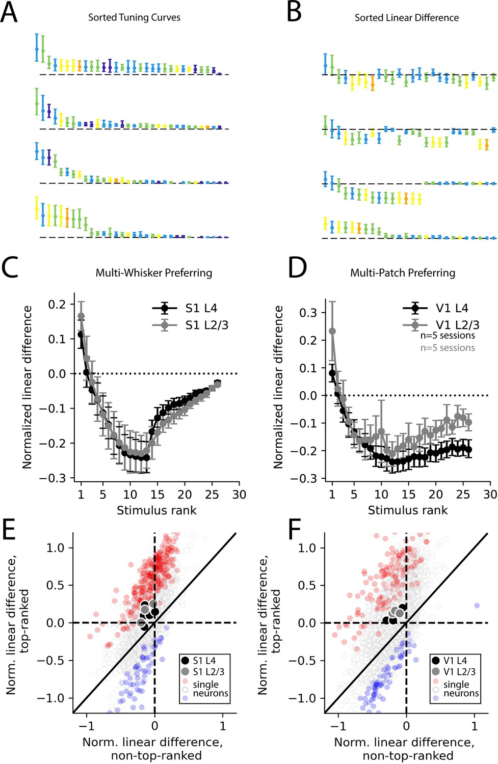
(A) Example V1 layer 2/3 tuning curves of the four multi-patch preferring neurons reproduced from Figure 4C, sorted by descending response magnitude. (B) Linear difference of the same neurons’ multi-patch stimulus responses, sorted as in (A). (C) Sorted linear difference averaged across neurons that preferred a multi-whisker stimulus in S1 L4 and L2/3. (D) Same as (C) for V1 L4 and L2/3. (E) Scatter plot of linear differences for preferred (top-ranked) stimulus versus an average of all non-preferred (non-top-ranked) stimuli, for individual neurons (small dots) and for averages across all neurons in an imaging session (large dots) for all S1 recordings. For single neurons, red color indicates significantly more supra-linear response to the top-ranked stimulus, compared to non-top-ranked stimuli, and blue color indicates significantly more sub-linear response (each p<0.01, using bootstrap resampling). (F) Same as (E), but for all V1 recordings. In all imaging sessions in both cortical areas, average supra-linearity is greater for the top-ranked stimulus than for non-top-ranked stimuli.
Figure 5—figure supplement 1
Supra-linearity of response to preferred stimulus reflects true deviation from linearity.
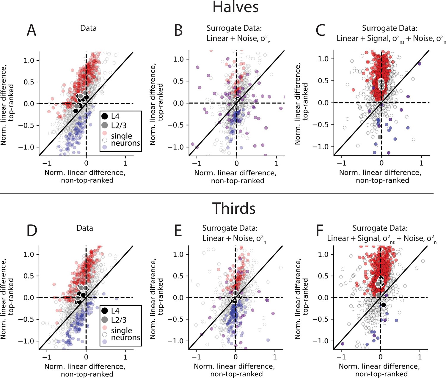
(A) Scatter plot of linear differences for preferred (top-ranked) stimulus versus an average of all non-preferred (non-top-ranked stimuli), for individual neurons (small dots), and for averages across all neurons in an imaging session (large dots) for all S1 recordings, reproduced from Figure 5E. (B) Same as (A), computed based on a surrogate dataset, in which the underlying tuning curve was constructed to reflect a linear sum of single-whisker responses. Stimulus-independent noise was added to each half of the data, such that the total variability across halves of the data was matched with the same quantity for the data linear differences. ‘Reliably estimated’ tuning curves were selected for display in the same way as for the actual data (see Materials and methods). (C) Same as (B), but for a surrogate dataset in which an identical stimulus-dependent signal was added to both halves of the data, such that the total variability across stimuli was matched with the same quantity for the data linear difference, as well as the stimulus-dependent noise in (B). (D–F) Same as (A–C), but operating on, or applying noise to, thirds of the data as in Figure 4—figure supplement 5. In all imaging sessions in both cortical areas, average supra-linearity is greater for the top-ranked stimulus than for non-top-ranked stimuli, whether splitting the data into halves or thirds.
Figure 5—figure supplement 2
Input-specific supra-linear integration is well captured by a simple linear-nonlinear transformation.
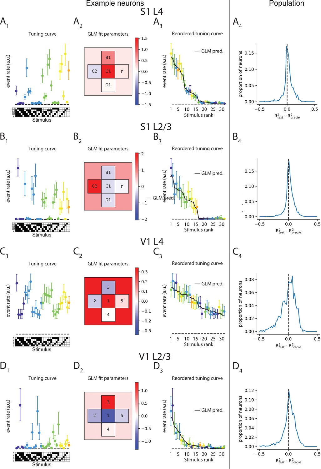
(A1) Example tuning curve of an S1 L4 neuron, plotted as in Figures 2 and 4. (A2) Best-fit generalized linear model parameters for the tuning curve in (A1), fit based on half of trials. Color corresponds to valuethe corresponding parameter, for individual whisker weights (small, labeled squares) and for bias term (background). (A3) Stimuli are ordered based on generalized linear model (GLM)-predicted response, which is plotted alongside the tuning curve values computed on the remaining half of trials. (A4) Test-set R2 of GLM fits is compared with the test-set R2 of an ‘oracle’ model, in which tuning curve values in the training set are used to predict tuning curve values in the test set directly. GLM fits significantly outperform the ‘oracle’ model on average in each case (p<10–4, Wilcoxon signed-rank test). (B–D) Same as (A), but for S1 L2/3, V1 L4, and V1 L2/3 neurons, respectively.
Videos
Video 1
Video of tactile stimulation with the novel, multi-piston tactile stimulator for head-fixed, locomoting mice.
Video 2
High speed tracking of whiskers and contacts during tactile stimulation.
Additional files
Download links
A two-part list of links to download the article, or parts of the article, in various formats.
Downloads (link to download the article as PDF)
Open citations (links to open the citations from this article in various online reference manager services)
Cite this article (links to download the citations from this article in formats compatible with various reference manager tools)
Synthesis of a comprehensive population code for contextual features in the awake sensory cortex
eLife 10:e62687.
https://doi.org/10.7554/eLife.62687


