A neural circuit for flexible control of persistent behavioral states
- Picower Institute for Learning & Memory, Department of Brain & Cognitive Sciences, Massachusetts Institute of Technology, United States
- MIT Biology Graduate Program, Massachusetts Institute of Technology, United States
Figures
Figure 1 with 8 supplements

Circuit-wide calcium imaging reveals a stable, low-dimensional neural representation of foraging states.
(A) (Top) Movement trajectory of a C. elegans animal foraging on bacterial food under the tracking microscope. Red and black dots mark the beginning and end of the trajectory, respectively. Orange indicates that the animal was in the roaming state, while blue indicates the animal was in dwelling state. (Bottom) The speed of the animal during the same period. (B) Putative neural circuit that mediates the sensory control of the roaming and dwelling states, based on the C. elegans connectome and genetic analyses from a previous study (Flavell et al., 2013). Each C. elegans neuron has a three-letter name. Blue highlights indicate sites of serotonin signaling and orange highlights indicate sites of PDF signaling. Gray arrows are synapses from the C. elegans connectome. The thickness of these arrows indicate the number of synapses at a given connection. Dotted blue and orange arrows indicate neuromodulatory connections from Flavell et al., 2013. (C) Example dataset from multi-neuron calcium imaging in a free-moving wild-type animal. The calcium activity of each neuron is shown in black. The green-red heat map in the background indicates axial velocity of the animal, and the behavioral state of the animal is shown on top. GCaMP6m data were divided by co-expressed mScarlett fluorescence levels and normalized to a 0–1 scale, based on the 1st and 99th percentiles of the neuron’s signal (see Materials and methods). (D) Event-triggered averages of individual neuron activity aligned to transitions between roaming (‘R’) and dwelling (‘D’) (left column), or transitions between forward runs (‘F’) and reversals (‘RV’) (right column). Data are shown as means and 95 % confidence interval (95% CI). (E) Histograms of individual neuron’s activity during roaming (orange), dwelling (blue), forward runs (green), or reversals (red). Note that shifts of distributions to the right indicate increased neural activity. (F) Simultaneously recorded activity of the 10 neurons projected onto the space spanned by the 1st and 2nd principal components (i.e. PC1 and PC2). Individual data points are colored according to the ongoing axial velocity. Histograms above and to the right of the scatterplot indicate distribution of PC1 and PC2 values for 3 ranges of axial velocity (): ≤ –0.0165 mm/s (red), –0.0165 mm/s < ≤ 0.0165 mm/s (gray), ≥ 0.0165 mm/s (green). (G) Projection of neural activity in principal component space, colored by the ongoing foraging state. Histograms show distributions of PC1 or PC2 values conditioned on the foraging state. (H) Comparison of measured velocity (x-axis) to the velocity predicted by a General Linear Model that was trained from the neural data (y-axis). The density of datapoints in this space is represented as a two-dimensional histogram. (I) Average Receiver Operating Curves from logistic regression models trained to predict foraging states using ongoing neural activity data from all 10 neurons or subsets of neurons (see Supplemental Methods for details). Dotted line indicates level expected by chance. Data in D-H are from the same set of wild-type animals (N = 17). *p < 0.05, **p < 0.01, ***p < 0.001, ****p < 0.0001, Wilcoxon rank-sum test.
Figure 1—figure supplement 1
Design and calibration of the spinning-disk confocal tracking scope.
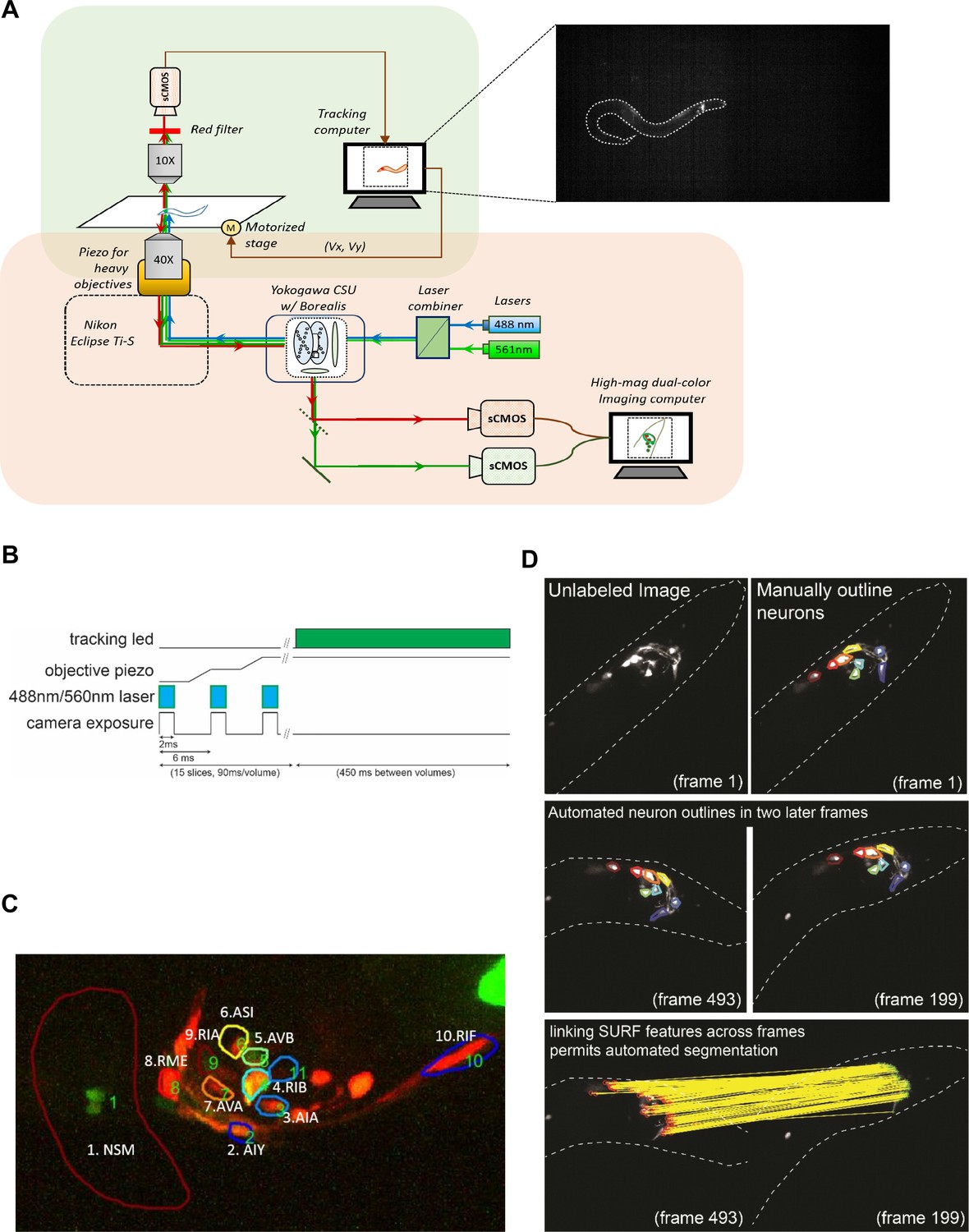
(A) Design of the microscope. Orange and green-shaded boxes indicate the confocal and behavioral tracking parts of the microscope, respectively. An example image from the behavior tracking camera is shown, with the worm outlined in white. mScarlett-expressing neurons can be robustly detected in the animal’s head. (B) To minimize photo-bleaching, movement artifacts, and animal disturbance, the laser illumination of animals was timed to camera exposure and objective piezo movement during volume acquisition, as is illustrated. The tracking LED was also only illuminated in between GCaMP/mScarlett volume acquisitions, so as to prevent cross-talk between the upper and lower microscope paths. Laser illumination permitted animal tracking during volume acquisition. (C) A sample volume captured by the confocal microscope. Neurons expressing the GCaMP6m and the mScarlett fluorescent proteins are annotated. For AIY, the neurite is labeled. (D) Semi-automated segmentation of neuron boundaries using the SURF algorithm. For a subset of frames in a video, the neuron boundaries are manually outlined. Then, the boundaries are propagated from one frame to others, based on image transformations that are defined by matching SURF features across frames.
Figure 1—figure supplement 2
Calibration of behavioral tracking accuracy and the effect of motion on calcium imaging data.
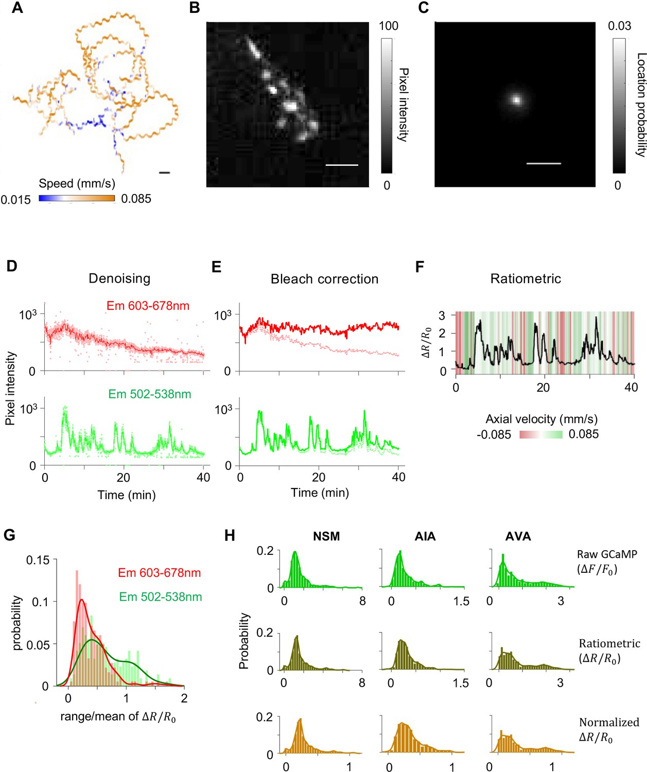
(A) Example trajectory of an animal recorded under the tracking confocal microscope. (B) An image of this animal’s head region captured through the behavior tracking camera. Bright pixels correspond to neurons expressing the mScarlett transgene. (C) Probability distribution of the location of the head region as seen through the behavior tracking camera across all of the frames of the recording shown in (A). All scale bars in (A–C) represent 0.1 mm. (D–F) Extraction of calcium activity from dual-channel fluorescent intensities from a representative neuron. (D) Time series of red (emission wavelength 603–678 nm) and green (emission wavelength 502–538 nm) fluorescent intensities were first denoised by median filtering. (E) Next, photobleaching over time was corrected by fitting and then normalizing away an exponential decay function. (F) Finally, the time series data from the green channels was divided by that from the red channel. The resulting time series was normalized to a relative scale of 0–1, with 0 corresponding to the 1st percentile and 1 to the 99th percentile of ratiometric values. (G) Range of variation normalized by mean calculated for the bleach-corrected red and green fluorescent intensities. Histograms were computed for aggregate data from all videos used in this study. Curved lines overlaying the red and green histograms (color matched) are mixture of Gaussian models fit to the corresponding histogram. (H) Distributions of fluorescence measurements are not perturbed by data processing. Probability distribution functions for the activity of three example neurons after various stages of data pre-processing: (top) cell-specific fluorescent signals from the green channel after denoising, bleach correction and baseline subtraction; (middle) ratiometric values computed by dividing signals from the green channel with those from the red channel; (bottom) normalized values computed by remapping the 1st and 99th percentiles of the distribution to 0 and 1.
Figure 1—figure supplement 3
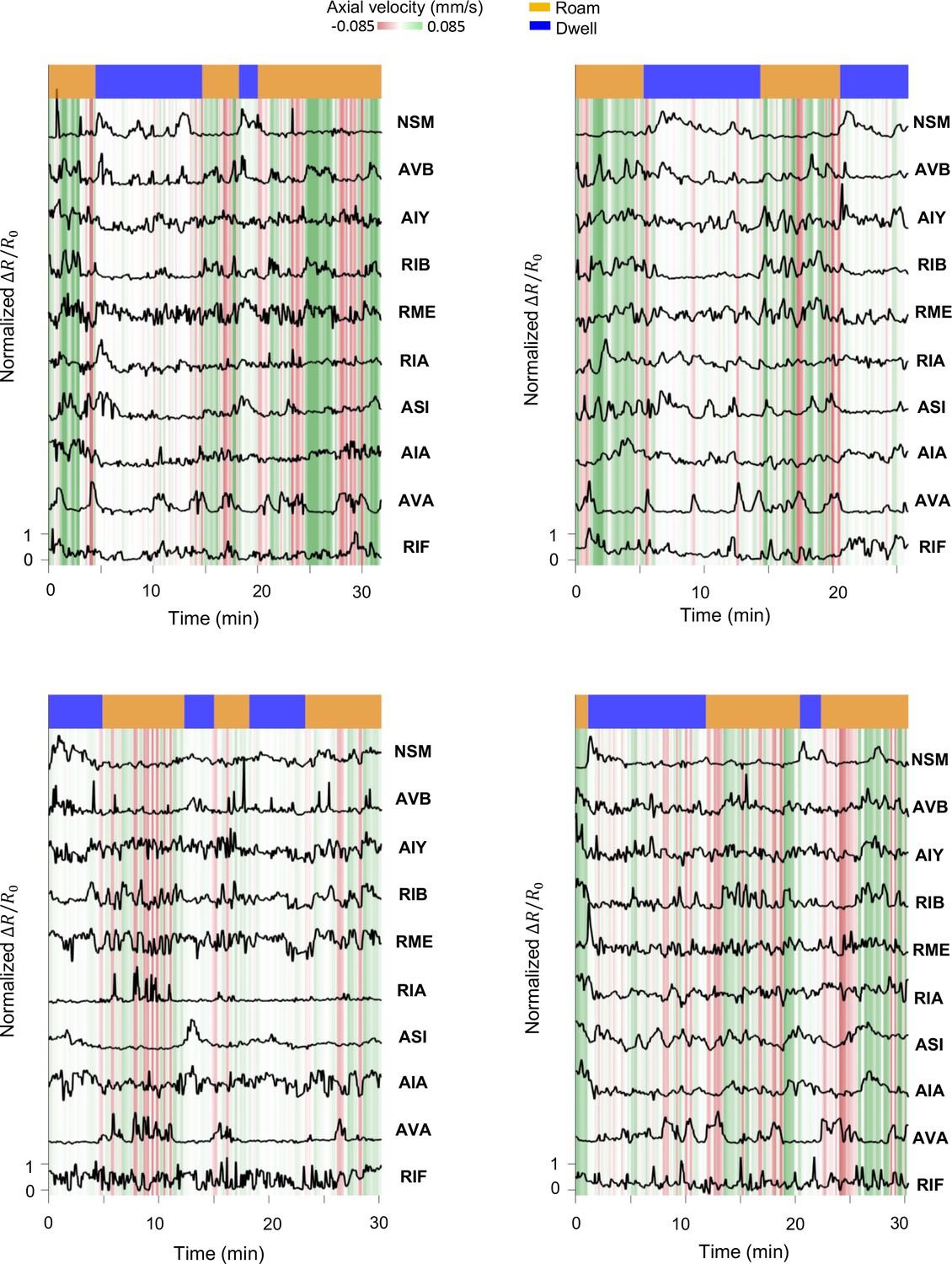
Additional examples of multi-neuron calcium activity traces in freely moving wild-type animals.
Data are shown as in Figure 1C.
Figure 1—figure supplement 4
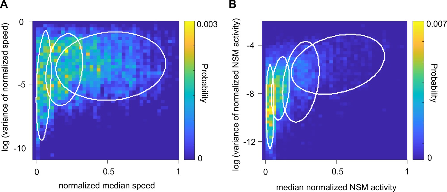
Gaussian Mixture Models (GMM) for analyzing animal speed and NSM calcium activity.
(A) GMM fit to the joint distribution of the normalized animal speed and the log-transformed variance of the normalized speed. Regions encircled by the white lines are centered on and encompass 50 % of the probability mass of each of the 3 Gaussians that compose of the GMM. (B) GMM fit to the joint distribution of the normalized NSM calcium activity and the log-transformed variance of it. Regions encircled by the white lines are centered on and encompass 50 % of the probability mass of each of the 4 Gaussians that compose the GMM.
Figure 1—figure supplement 5

Encoding of behavioral parameters by the calcium activity of individual neurons.
(A) Joint distribution of individual neuron’s activity versus axial velocity (left column) or speed (right column). Colored dots indicate the Spearman’s correlation coefficient between neural activity and the locomotory parameters for all wild-type data or conditioned on the animal’s movement direction. Green and red color indicates positive or negative correlation respectively, while the size the dot indicates the magnitude of the correlation coefficient. Insignificant correlations are represented with a small black dot. (B) Average autocorrelation function for the activity of each neuron across wild-type animals. The average autocorrelation function for animal speed is shown in green for comparison. N = 17 wild-type animals, same dataset as in Figure 1.
Figure 1—figure supplement 6
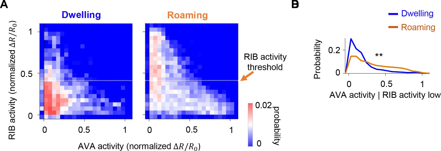
Differences in RIB and AVA joint activity during roaming compared to dwelling.
(A) Joint distributions of AVA and RIB activity during dwelling and roaming in wild-type animals. (B) Quantification of data from panel (A). Distribution of AVA activity, conditioned on RIB activity being low, during roaming versus dwelling. **p < 0.01, Wilcoxon rank-sum test.
Figure 1—figure supplement 7

Relationships between specific neurons and the principal components.
(A) Loadings of individual neurons on to PCs 1–4. (B) Projection of neural activity in principal component space, colored by the concurrent activity of each of the 10 neurons. N = 17 WT animals, same dataset as in Figure 1.
Figure 1—figure supplement 8

Examples showing the prediction of locomotion parameters using circuit activity.
Prediction of foraging state (top ethograms) and axial velocity (middle traces) from the simultaneous activity of the 10 neurons shown in Figure 1. Model predictions were plotted side-by-side with measured data for comparison. Activity traces of NSM and AVA were plotted to illustrate the multi-neuron activity data used for prediction.
Figure 2 with 1 supplement
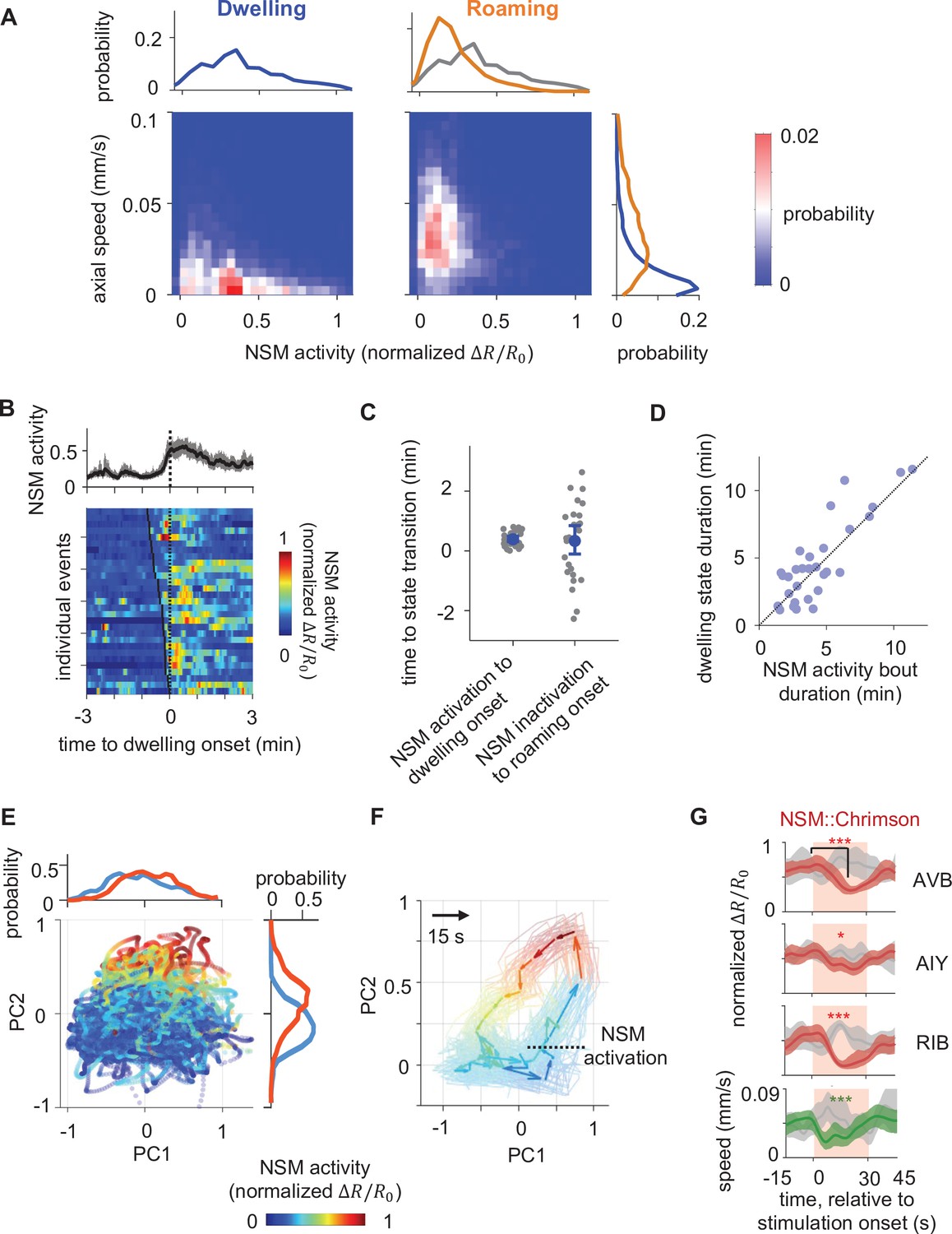
Persistent NSM activity is associated with the dwelling state.
(A) Joint distribution of NSM activity and the concurrent axial velocity during the dwelling (left column) or the roaming (right column) state. Histograms on top show marginal distributions of NSM activity during dwelling (left) or roaming (right). Histogram to the right show marginal distributions of axial velocity during dwelling (blue) or roaming (orange) states. (B) NSM activity aligned to the onset of dwelling states. (Top) Average NSM activity around the onset of dwelling states. (Bottom) Heat map of NSM activity around individual instances of roaming-to-dwelling transitions. Dotted black line denotes the onsets of dwelling states. Black ticks on the heat map mark the onset of an NSM activity bout. (C) Left: latencies of roaming-to-dwelling transitions relative to the closest onset of an NSM activity bout. Right: latencies of dwelling-to-roaming transitions relative to the closest offset of an NSM activity bout. NSM activity bouts are defined through Gaussian Mixture Clustering (see Methods for details). (D) Scatterplot of the durations of individual dwelling states and the durations of their coinciding NSM activity bouts. (E) Projection of neural activity in principal component space, colored by concurrent NSM activity. Histograms show distributions of NSM activity along both axes. (F) Average circuit activity dynamics in principal component space aligned to the onset of NSM activation. Each colored arrow represents average activity dynamics over a 15 s interval. Color indicates ongoing NSM activity. Faint lines show bootstrap samples of the average dynamics. (G) Event triggered averages of individual neuron activity and animal speed aligned to the optogenetic activation of NSM. Red and green traces represent data from animals raised on all-trans retinal (ATR) (N = 6 animals), while gray traces represent data from control animals raised without ATR (N = 4 animals). Light red patch indicates the time window in which the red light is turned on. Comparisons are made between 1 s before the onset of the red light stimulation and 18 s into the stimulation. Data are shown as means and 95% C.I.s **p < 0.01, ***p < 0.001, ****p < 0.0001, Wilcoxon rank-sum test with Benjamini-Hochberg (BH) correction.
Figure 2—figure supplement 1
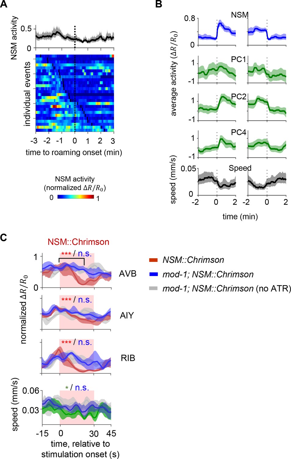
Further analysis of NSM activity.
(A) NSM activity aligned to the onset of roaming states. (Top) Average NSM activity around the onset of roaming states. (Bottom) Heat map of NSM activity around instances of dwelling-to-roaming transition. Same color scale as in (D). Dotted black line denotes the onset of roaming states. Black ticks on the heat map mark the offset of an NSM activity bout. (B) Event-triggered averages centered on NSM activation (left) and termination (right) events. Data are from 17 WT animals and are shown as mean and 95% CI. PC4 is shown as an example to illustrate that dynamics beyond the first two principle components also change around the time of NSM activation. (C) Event triggered averages of individual neuron activity and animal speed aligned to the optogenetic activation of NSM for the indicated genotypes and experimental conditions. Light red patch indicates the time window in which the red light is turned on. Comparisons are made between 1 s before the onset of the red light stimulation and 22 s into the stimulation. N = 4–5 animals per condition, with an average of three independent stimulation events (minutes apart) per animal. Wild-type control animals were recorded in parallel to mod-1 mutants. Data are shown as means and 95% C.I.s *p < 0.05, **p < 0.01, ***p < 0.001, ****p < 0.0001, Wilcoxon rank-sum test with Benjamini-Hochberg (BH) correction.
Figure 3 with 2 supplements

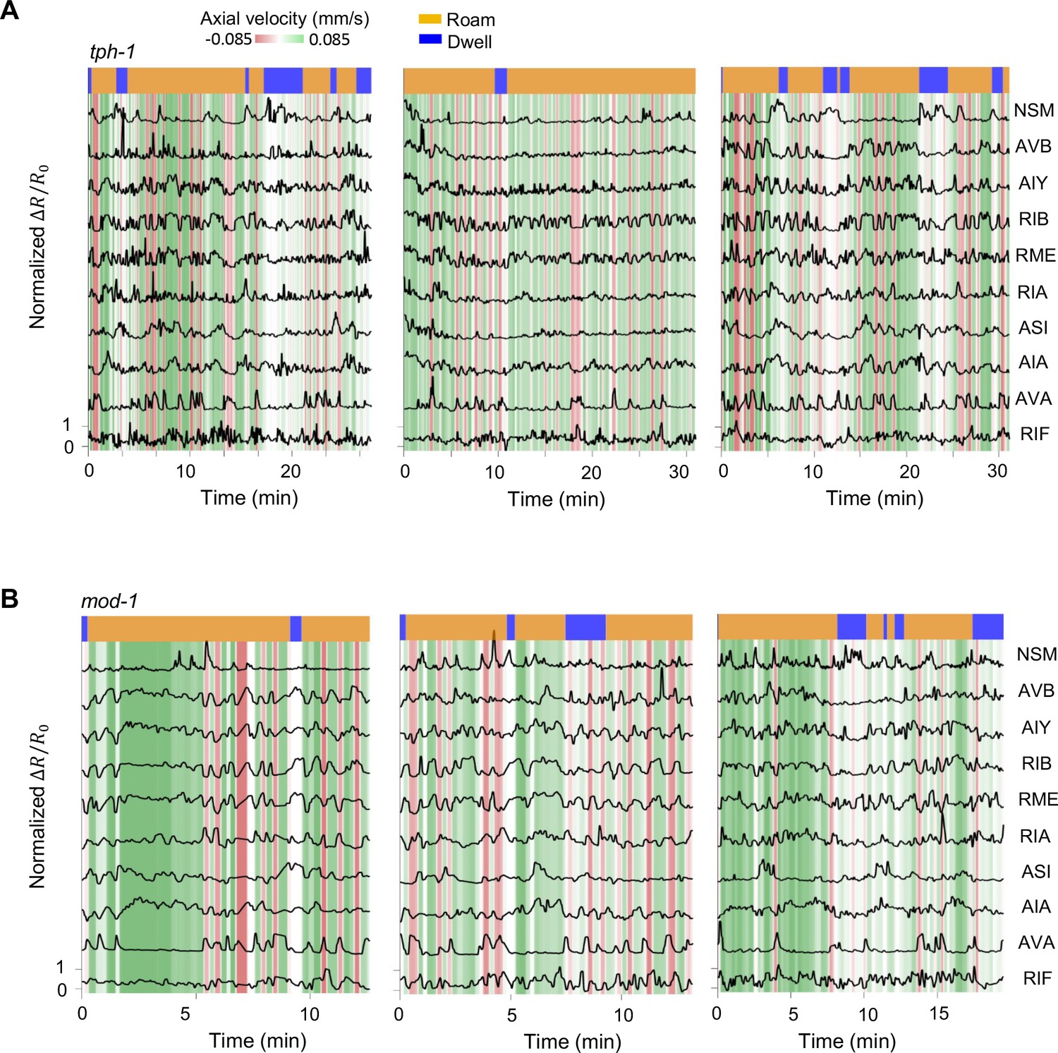
Serotonin signaling promotes persistent activation of serotonergic NSM neurons via a mutual inhibitory circuit.
(A–B) Example circuit-wide calcium imaging datasets from tph-1 (A) and mod-1 (B) mutant animals, shown as in Figure 1C. (C) Association of NSM activity and axial speed in the indicated genotypes. Data are shown as probability density plots. (D) Duration of NSM activity bouts for the indicated genotypes. Data points represent individual NSM activity bouts and violin plots show distributions across animals of the same genotype. Blue ‘+’ marks the median of each distribution. (E) Probability of NSM being active in wild type animals and serotonin mutants. Data points represent individual animals and violin plots show distributions across animals of the same genotype. Blue ‘+’ marks the median of each distribution. For (D–E), N = 17, 10, and 8 animals for WT, tph-1, and mod-1, respectively. (F) Event triggered averages of NSM activity and animal speed aligned to the optogenetic activation of mod-1 expressing neurons. Red and green traces represent data from animals raised on all-trans retinal (ATR) (N = 7 animals), while gray traces represent data from control animals raised without ATR (N = 4 animals). Data are shown as means and 95% C.I.s. Light red patch indicates the time window in which the red light is turned on. For NSM calcium activity, the comparison is made between 1 s before the onset of the red light stimulation and 30 s into the stimulation. For animal speed, the comparisons is made between 1 s before the onset of the red light stimulation and 60 s into the stimulation. (G) Circuit schematic based on results from the tph-1 and mod-1 mutants, showing cross inhibition between the NSM and the MOD-1 expressing neurons. For (D–F), **p < 0.01, ***p < 0.001, ****p < 0.0001, Wilcoxon rank-sum test with Benjamini-Hochberg (BH) correction.
Figure 3—figure supplement 1

Further analysis of NSM activity.
(A) Fraction of time animals spent roaming versus dwelling for wild-type (WT), tph-1, and mod-1 animals. Data points represent individual animals and violin plots show distributions across animals of the same genotype. Blue ‘+’ marks the median of each distribution. N = 17, 10, and 8 animals for WT, tph-1, and mod-1, respectively. **p < 0.01, ***p < 0.001, ****p < 0.0001, Wilcoxon rank-sum test with Benjamini-Hochberg (BH) correction.
Figure 3—figure supplement 2
Additional examples of multi-neuron calcium activity traces in free-moving serotonin mutants.
Data are shown as in Figure 1C.
Figure 4 with 5 supplements
PDF signaling is required for mutual exclusivity between circuit states and acts downstream of the 5-HT target neurons in the mutual inhibitory circuit.
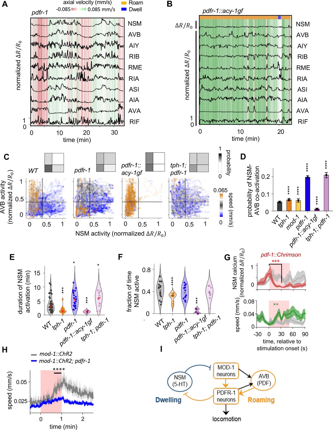
(A) Example circuit-wide calcium imaging dataset from pdfr-1 mutants lacking PDF neuropeptide signaling, shown as in Figure 1C. No roaming/dwelling ethogram is shown for pdfr-1 animals due to changes in their speed distribution that implicate altered or new behavioral states (see Figure 4—figure supplement 4A-B). (B) Example circuit-wide calcium imaging dataset from transgenic animals expressing the hyperactive PDFR-1 effector ACY-1(P260S) specifically in pdfr-1 expressing neurons. For NSM, the un-normalized is shown since the values never exceeded 10 % of the average peak NSM activity wild-type animals. (C) Scatterplots of NSM and AVB activity in pdfr-1 mutants, transgenic pdfr-1::acy-1(P260S)gf animals, and tph-1; pdfr-1 double mutants. Data points are colored by the instantaneous speed of the animal. Color scale was chosen so that blue colors correspond to speeds typical of the dwelling state, orange correspond to speeds typical of the roaming states, while gray colors indicate speeds in-between the former. Dotted lines show the threshold values for NSM and AVB activity used for defining ‘co-activity’ (determined using the Otsu method; see Methods). Insets show the density of data points in each of the quadrants defined by these threshold activity levels. (D) Probability of NSM and AVB being co-active for genotypes shown in (C). ***p < 0.001; ****p < 0.0001, bootstrap estimates of the mean with BH correction. (E) Duration of NSM activity bouts for the indicated genotypes. Data points corresponds to individual NSM activity bouts. Each violin plot represent data from animals of the same genotype.’+’ denotes the median of each distribution. (F) Probability of NSM being active in wild-type and mutant animals. Data points corresponds to individual NSM activity bouts. Each violin plot represent data from animals of the same genotype. ‘+’ denotes the median of each distribution. For (C–F), N = 17, 10, 8, 11, 9, and 8 animals for WT, tph-1, and mod-1, pdfr-1, pdfr-1::acy-1gf, and tph-1;pdfr-1 animals. (G) Event triggered averages of NSM activity and animal speed aligned to the optogenetic activation of pdf-1 expressing neurons. Red and green traces represent data from animals raised on all-trans retinal (ATR) (N = 5 animals), while gray traces represent data from control animals raised without ATR (N = 4 animals). Data are shown as means and 95% C.I.s. For NSM calcium activity and animal speed, comparisons are made between 1 s before the onset of the red light stimulation and 30 s into the stimulation. (H) Speed of wild-type and pdfr-1 mutant animals in response to optogenetic activation of the MOD-1 expressing neurons (red shading). Average speeds during the window spanned by the black line were compared between animals of the two genotypes. (I) Circuit schematic summarizing results shown in (C–H): the PDFR-1 expressing neurons act downstream of the MOD-1 expressing neurons to inhibit the 5-HT neuron NSM. Black arrows indicate anatomical connections based on the C. elegans connectome (White et al., 1986). For (D- H), **p < 0.01, ***p < 0.001, ****p < 0.0001, Wilcoxon rank-sum test with BH correction.
Figure 4—figure supplement 1
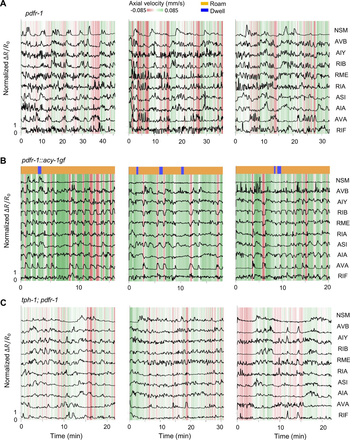
Additional examples of multi-neuron calcium activity traces in free-moving serotonin mutants.
Data are shown as in Figure 1C.
Figure 4—figure supplement 2
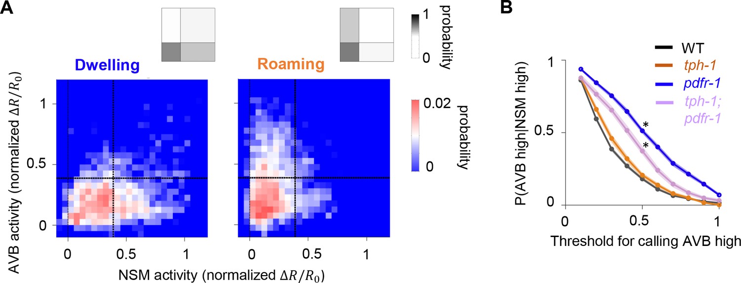
Further analysis of NSM-AVB co-activity.
(A) Joint distribution of NSM and AVB activity during roaming and dwelling. (B) Data from the indicated genotypes, showing the probability of AVB activity exceeding a range of different threshold values, while NSM activity is high. Note that in WT (black) there is a rapid decrease in P(AVB high | NSM high) as the threshold for calling AVB high is increased. This reflects a low incidence of high AVB activity during high NSM activity, which is attenuated in pdfr-1 mutants. Error bars show boostrapped 95 % confidence intervals *p < 0.05, empirical bootstrap test versus wild-type.
Figure 4—figure supplement 3
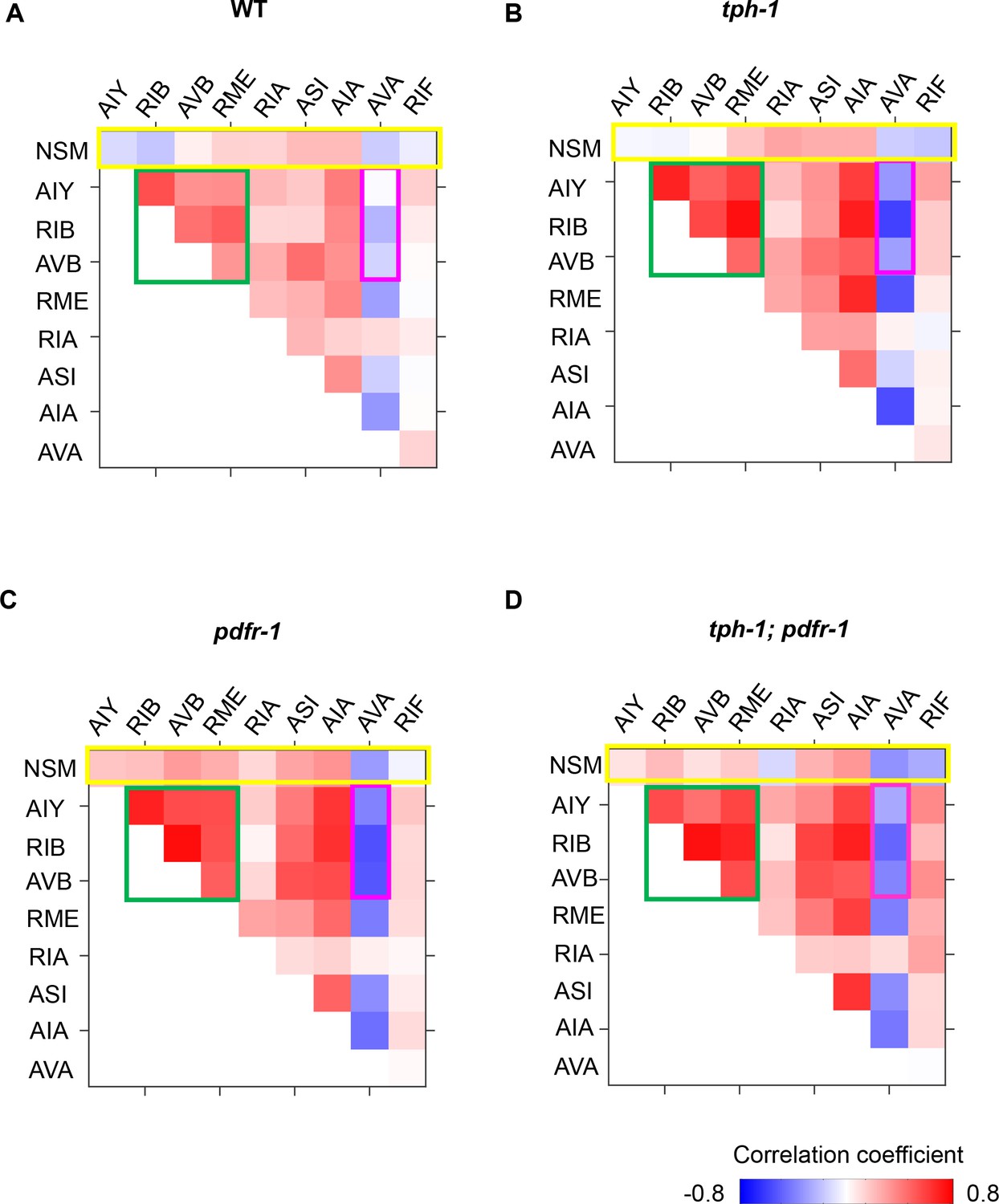
Correlations between neurons in wild-type and mutant animals.
(A–D) Pairwise correlation coefficients among neurons in the roaming-dwelling circuit. Same color scale (lower right) is used to represent correlation coefficients. Boxes outline the neurons known to promote forward runs (green) and reversals (magenta), as well as the correlations of NSM and other neurons (yellow). N = 17, 10, 8, 11, and 8 animals for WT, tph-1, and mod-1, pdfr-1, and tph-1;pdfr-1 animals.
Figure 4—figure supplement 4
Joint activity of NSM and AVB in serotonin and PDF signaling mutants.
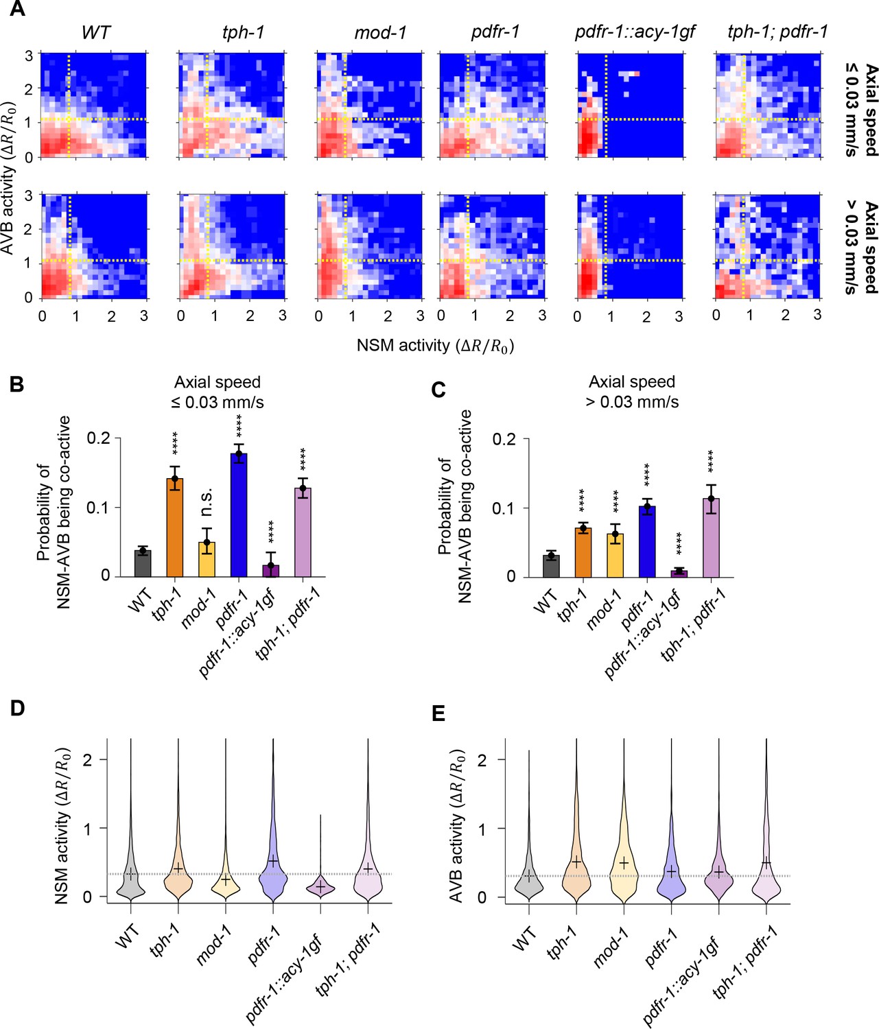
(A) Joint distribution of NSM and AVB activity, without normalizing to a 0–1 scale, for movement speeds below (top row) or above (bottom row) a speed of 0.03 mm/s. (B–C) Probability of NSM and AVB being coactive for wild-type and mutant animals moving below (B) or above (C) 0.03 mm/s, quantified without using the 0–1 normalization method. (D–E) Distributions of NSM (D) and AVB (E) activity, without normalizing to a 0–1 scale, across wild-type and mutant animals. N = 17, 10, 8, 11, and 8 animals for WT, tph-1, and mod-1, pdfr-1, and tph-1;pdfr-1 animals. ***p < 0.001, ****p < 0.0001, Wilcoxon rank-sum test with Benjamini-Hochberg (BH) correction.
Figure 4—figure supplement 5
Analyses of circuit dynamics and foraging behavior in serotonin and PDF signaling mutants.
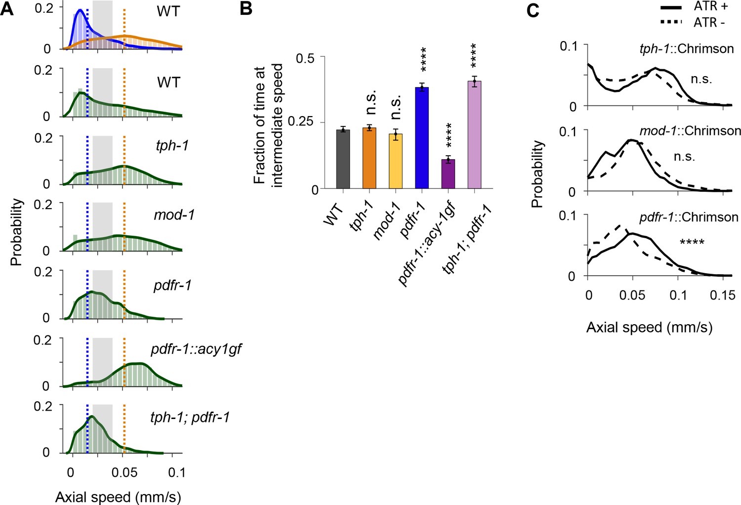
(A) Distributions of axial speed in wild-type animals and various 5-HT and PDF signaling mutants. Top panel shows speed distributions specific to the dwelling (blue) or the roaming (orange) states. Dotted blue and orange lines indicate the median speeds for the dwelling and roaming states, respectively. Shaded region defines the intermediate speed range used for the analysis in panel B. (B) Fraction of time animals moved at speeds intermediate between typical dwelling and roaming speeds for wild-type and mutant animals. The range of intermediate speeds is defined by the shaded region shown in panel B. Data are shown as mean and standard error. N = 17, 10, 8, 11, 9, and 8 animals for WT, tph-1, and mod-1, pdfr-1, pdfr-1::acy-1gf, and tph-1;pdfr-1 animals. ***p < 0.001, ****p < 0.0001, Wilcoxon rank-sum test with Benjamini-Hochberg (BH) correction. (C) Distributions of axial speed during spontaneous locomotion in transgenic animals used for optogenetic experiments in Figures 2G—4 grown on (solid line) or off (dotted line) ATR. *p < 0.05, **p < 0.01, ****p < 0.0001, comparison of bootstrap distributions with BH correction.
Figure 5 with 3 supplements
A CNN classifier identifies circuit activity patterns predictive of roaming-to-dwelling state transitions.
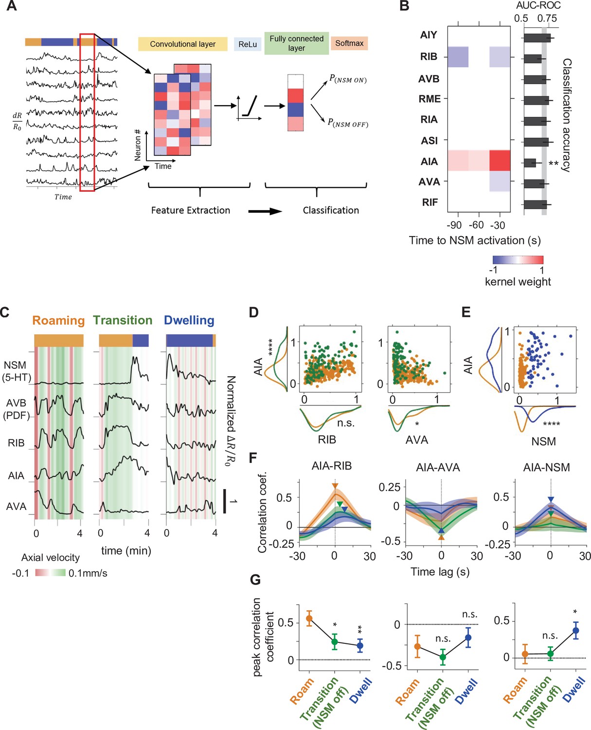
(A) Schematic illustrating the architecture of the Convolutional Neural Network (CNN) trained to predict NSM activation events. (B) Left: a common convolutional kernel found across successfully trained CNNs. Only weights that are significantly different from zero are colored. Right: Feature selection results. Each black bar depicts the average area under the curve for the Receiver Operating Characteristic curve (AUC-ROC) from networks trained using data with one neuron held out at a time. The identity of the held-out neuron is indicated to the far left. The gray stripe in the background denotes the 95% CI of the AUC-ROC from networks trained using data from all nine neurons. Error bars are 95% CI of the mean. **p < 0.01, bootstrap estimate of the mean with BH correction. (C) Example activity traces from NSM, AVB, and the three neurons with significant weights in the convolutional kernel. Activity traces were taken during roaming (left), dwelling (right) and roaming-to-dwelling transition. (D) Scatterplots of simultaneously measured neural activity of the indicated pairs of neurons. Orange data points are taken during roaming states at least 1 min before the onset of the next dwelling states and before NSM becomes active. Green data points are taken within 1 min before the onset of dwelling states. Along the x- and the y- axes are marginal probability distributions of the data points shown in the scatterplots. (E) Scatterplots of simultaneously measured neural activities of AIA and NSM. Orange data points are taken within 1 min before the onset of the next dwelling states and before NSM becomes active. Blue data points are taken within 30 s after the onset of dwelling states. Along the x- and the y- axes are marginal probability distributions of the data points shown in the scatterplots. (F) Average cross-correlation functions between the indicated pairs of neurons during roaming (orange, data taken from 100 to 70 s before the onset of the next dwelling state), roaming-to-dwelling transition (green, data taken from 30 to 0 s before the NSM activation event prior to the onset of the next dwelling state), or dwelling (blue, data taken from 10 to 40 s after dwelling onset). Error bars are standard error of the mean. Arrowheads denote the point of maximum in absolute magnitude of the cross-correlation function. (G) Average cross-correlation coefficients computed at peak points indicated in (F). For (B, D–G), N = 17 WT animals. For (D–E and G), *p < 0.05, **p < 0.01, ****p < 0.0001, Wilcoxon rank-sum test with BH correction.
Figure 5—figure supplement 1
Parameter selection for the CNN model.
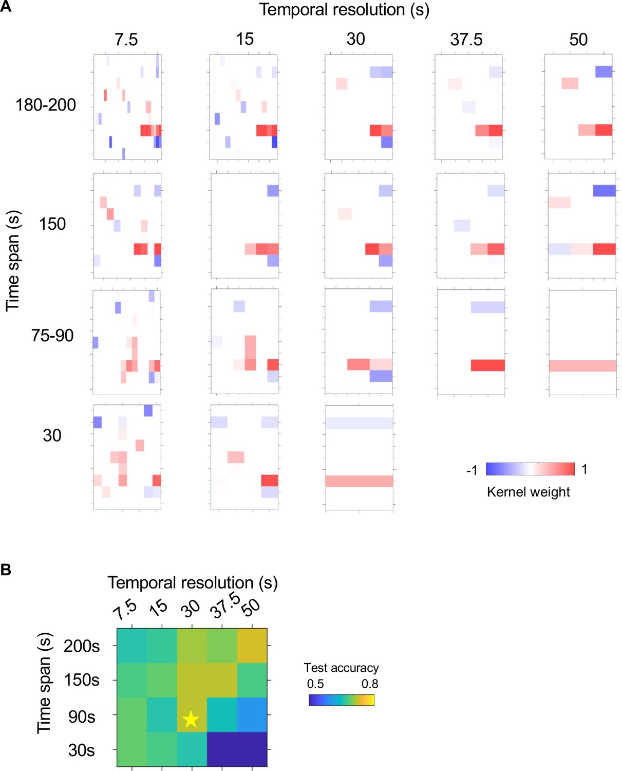
(A) Convolutional kernels from CNN models trained to predict NSM activation using neural activity history of different time span and diverse temporal resolution. Kernels in the same row are trained neural activity history that span similar durations prior to NSM activation; kernels in the same column are trained with activity data of identical temporal resolution. Each kernel corresponds to a boot-strapped average across training episodes. Only kernel weights significantly different from zero are represented by a blue-red color scale spanning from –1–1 (lower right). See Supplemental Methods for further details on model specification and training. (B) Average test accuracy of the model types presented in (A). Only models with a test accuracy greater than 0.5 (i.e. better than random guess) are included. The CNN architecture that uses input data span of 90 s at 30 s resolution was chosen for its simplicity and accuracy and used for further analysis in Figure 5 -S2. All models were trained using the same WT data as in Figure 5.
Figure 5—figure supplement 2
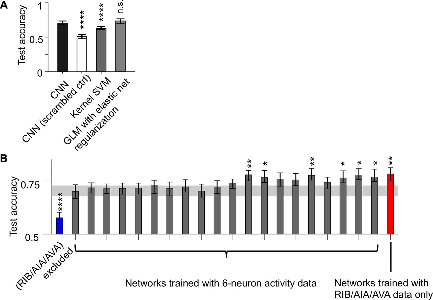
Evaluation of CNN classifier performance.
(A) AUC-ROC of the CNN classifiers trained on authentic data compared to those trained on scrambled data and to the performance of two other common types of classifiers. Data are shown as mean and 95% CI from 200 training sessions. (B) AUC-ROC of CNN classifiers trained on data withholding different neuron triplets from the full data set, or with data from only the RIB, AIA, and AVA neurons. Gray band indicates the 95% CI of the accuracy of CNN classifiers trained on the full data set, as shown in A.
Figure 5—figure supplement 3

Convolutional kernels trained to predict transitions in foraging state or NSM activity.
(A) Average convolutional kernels from CNN models trained to predict dwelling state onset using data from all neurons except (left panel) or including (right panel) NSM. Only kernel weights significantly different from zero are represented by a blue-red color scale spanning from –1–1. (B) Average convolutional kernels from CNN models trained to predict roaming state onset using data from all neurons except (left panel) or including (right panel) NSM, presented similarly as in (A). (C) Average convolutional kernel from CNN models trained to predict the offset of NSM activity bouts. All models were trained using the same WT data as in Figure 5.
Figure 6 with 1 supplement
The AIA sensory processing neuron can drive behavioral state switching.
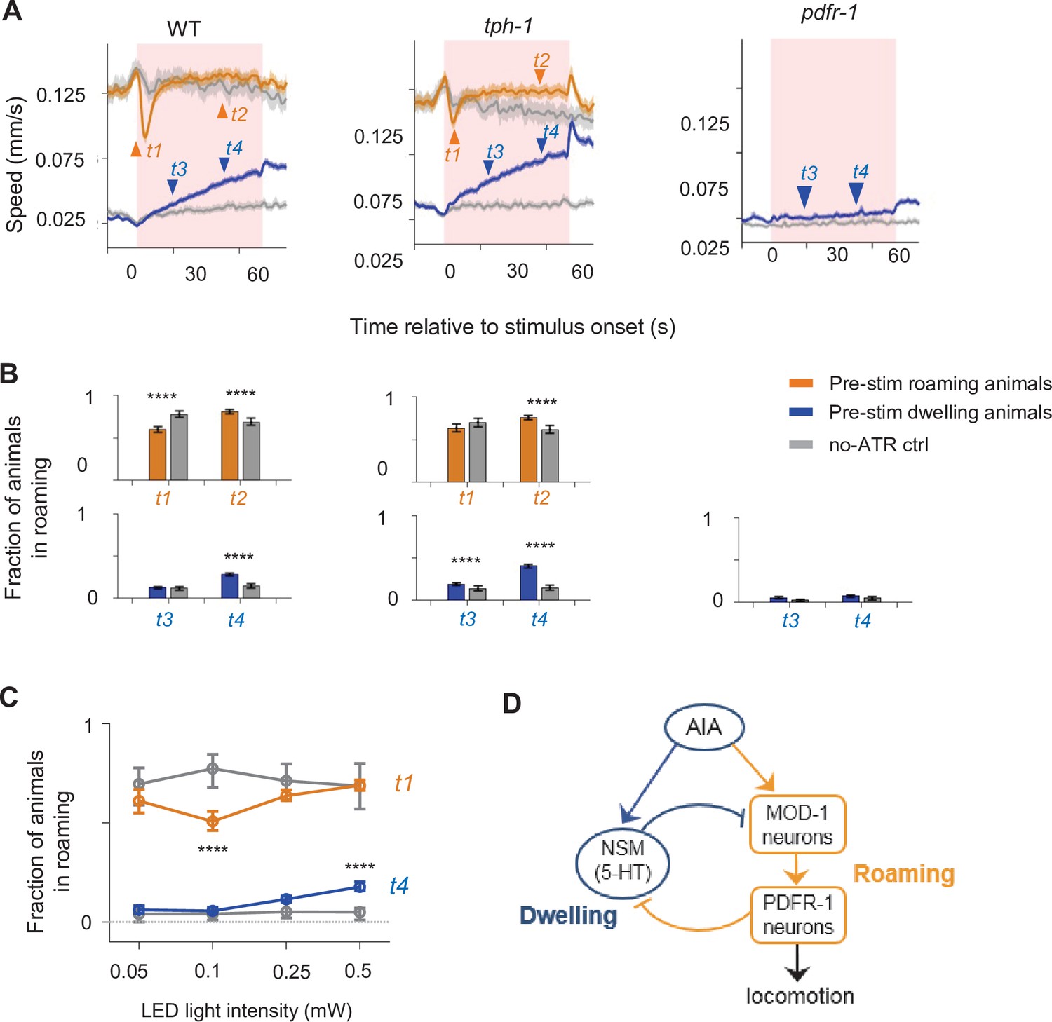
(A) Average locomotion speed before, during, and after AIA::Chrimson activation for wild-type (left), tph-1 (middle), and pdfr-1 (right) animals. Animals were grouped by whether they were roaming (orange) or dwelling (blue) prior to AIA stimulation. Pink patches in the background denote the one-minute stimulation window. Gray lines indicate no-all-trans-retinal (no-ATR) controls. N = 1,032 wild-type animals were compared to N = 370 no-ATR controls. N = 927 tph-1 mutants were compared to N = 284 no-ATR control. N = 383 pdfr-1 mutants were compared to N = 237 no-ATR controls. Note that roaming in pdfr-1 animals was too rare and brief to be included for analysis on AIA-induced slowing. Orange and blue arrowheads denote time points used for analyses in (B). Error bars are 95% CI of the mean. (B) Fraction of animals in the roaming state at different phases of AIA::Chrimson stimulation. Top: Among animals that were roaming pre-stimulation, the fraction of them that were roaming after 4 seconds or 40 seconds from the onset of AIA stimulation. Bottom: Among animals that were dwelling pre-stimulation, the fraction of them that were roaming after 20 seconds or 40 seconds from the onset of AIA stimulation. Same analyses were performed for wild-type (left), tph-1 (middle), and pdfr-1 (right) animals. See panel (A) for full traces. (C) AIA-induced changes in roaming and dwelling at different optogenetic stimulation intensities. For (B–C), error bars are 95% CI of the mean and ****P < 0.0001, Wilcoxon rank-sum test. (D) Functional architecture of the circuit controlling the roaming and dwelling states, based on results from Figures 2—5.
Figure 6—figure supplement 1

Connectivity of the AIA interneuron.
Synaptic inputs and outputs of the AIA neuron. Data are from the C. elegans connectome. Bilaterally symmetric pairs of neurons (e.g. AIAL and AIAR) were merged here for display purposes. Connections supported by only one single synapse were not included. Note the dense synaptic inputs onto AIA from chemosensory neurons.
Figure 7 with 1 supplement
The AIA sensory processing neuron can promote either roaming or dwelling, depending on the sensory context.
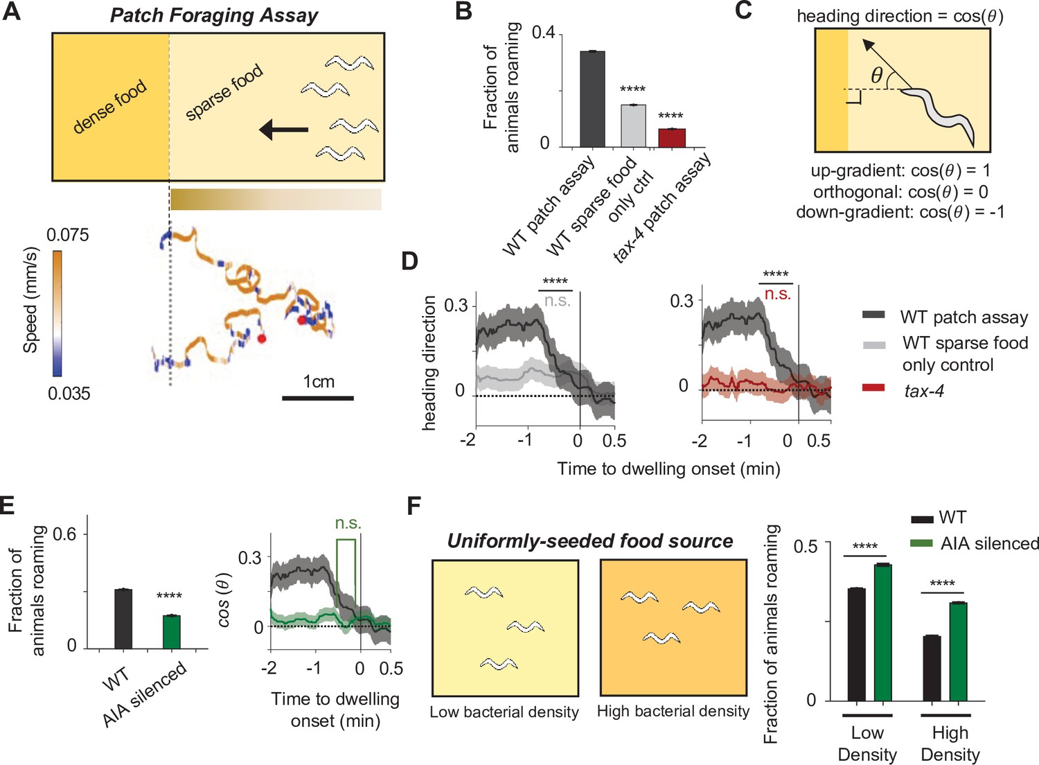
(A) Top: Cartoon depicting the patch foraging behavioral assay. Horizontal bar with gradient signifies the food odor gradient emanating from the dense food patch. Bottom: example trajectories of two animals from a patch foraging assay. Color scale indicates speed, with orange corresponding to roaming-like speeds and blue dwelling-like speeds. Red dots denote the starting points of the animals. (B) Average fraction of animals roaming on the sparse food patch in the patch foraging assay. Comparisons are made between wild-type animals in the patch foraging assay (n = 288), wild-type animals assayed on uniform sparse food with no dense patch around (n = 194), and tax-4 animals in the patch foraging assay (n = 81). (C) Schematic depicting how heading bias is calculated. (D) Event-triggered averages showing average heading bias of animals for two minutes prior to transitions into dwelling states. Experimental conditions are depicted with same color scheme as in (B). Data are shown as means ± SEM. The average heading bias within two time windows, one from 60 to 50 s prior to dwelling onset, the other from 20 to 10 s prior to dwelling onset, were compared. (E) Left: Average fraction of animals roaming on sparse food in the patch foraging assay in wild-type (black) versus AIA silenced (AIA::unc-103gf) animals (green). Right: Heading bias of AIA-silenced animals (green) two minutes prior to the transition into the dwelling state. n = 197. Wild-type data (black with gray error bar) are shown for comparison. (F) Left: schematic of behavioral assays in uniformly seeded food environments. Right: Average fractions of animals roaming for wild-type (black bars) and AIA-silenced (green bars) animals exposed to two different densities of uniformly distributed sparse food. For all calculations on fraction of animals roaming, error bars are 95% CI of the mean. For all calculations of heading bias, error bars are SEM. For all comparisons, **p < 0.01, ****p < 0.0001, Wilcoxon rank sum test with BH correction.
Figure 7—figure supplement 1
Food-directed navigation in patch foraging assays.
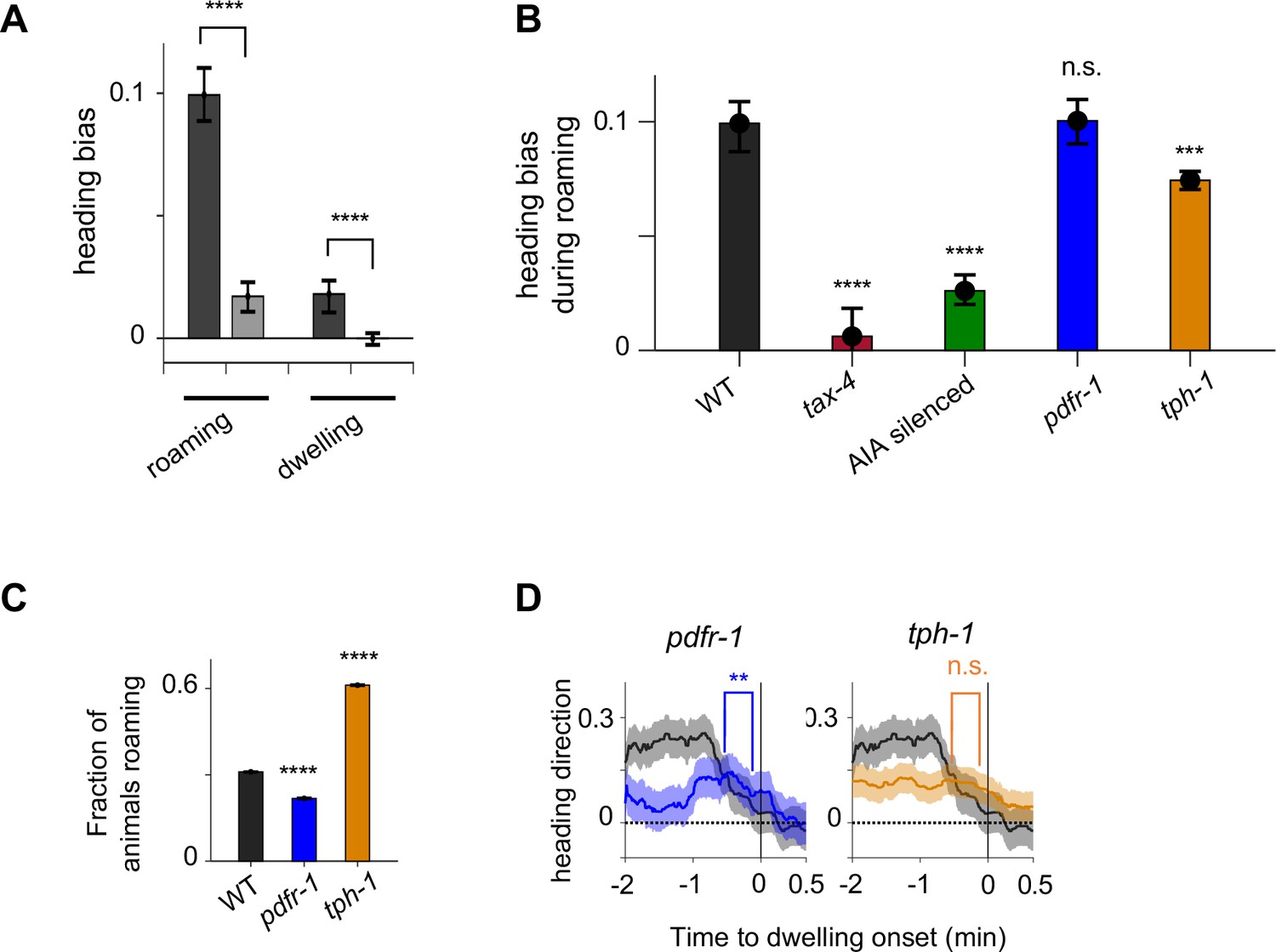
(A) Heading bias during roaming versus dwelling in the patch foraging assay (dark bars) and control sparse food plates (light bars), shown separate for roaming and dwelling. (B) Heading bias during roaming for animals of the indicated genotypes. (C) Average fractions of animals roaming on the sparse food patch for pdfr-1 (blue) and tph-1 (orange) mutant animals during the patch foraging assay. (D) Heading bias two minutes prior to the transition into the dwelling state for pdfr-1 (blue) and tph-1 (orange) mutant animals. n = 99 for pdfr-1 and n = 212 for tph-1 animals. Wild-type data (black with gray error bar) are shown for comparison. All error bars are 95% CI of the mean. ***p < 0.001, ****p < 0.0001, Wilcoxon rank sum test.
Tables
Key resources table
| Reagent type (species) or resource | Designation | Source or reference | Identifiers | Additional information |
|---|---|---|---|---|
| Strain, strain background (C. elegans) | N2 | CGC | ID_FlavellDatabase: N2 | Wild-type Bristol N2 |
| Strain, strain background (C. elegans) | SWF90 | This study | ID_FlavellDatabase: SWF90 | flvEx46[[tph-1::GCaMP6m, mod-1::GCaMP6m, sto-3::GCaMP6m, glr-3::GCaMP6m, odr-2b::GCaMP6m, gcy-28.d::GCaMP6m, lgc-55(short)::GCaMP6m, nmr-1::GCaMP6m, tph-1::wrmScarlett, mod-1::wrmScarlett, nmr-1::wrmScarlett, sto-3::wrmScarlett]; lite-1(ce314), gur-3(ok2245)].See: Figure 1. |
| Strain, strain background (C. elegans) | SWF113 | This study | ID_FlavellDatabase: SWF113 | flvIs1[tph-1::GCaMP6m, mod-1::GCaMP6m, sto-3::GCaMP6m, glr-3::GCaMP6m, odr-2b::GCaMP6m, gcy-28.d::GCaMP6m, lgc-55(short)::GCaMP6m, nmr-1::GCaMP6m, tph-1::wrmScarlett, mod-1::wrmScarlett, nmr-1::wrmScarlett, sto-3::wrmScarlett]; lite-1(ce314), gur-3(ok2245).See: Figures 1—5, Figure 1—figure supplements 1–8, Figure 2—figure supplement 1, Figure 3—figure supplement 1, Figure 4—figure supplements 2–5, Figure 5—figure supplements 1–3. |
| Strain, strain background (C. elegans) | SWF186 | This study | ID_FlavellDatabase: SWF186 | flvIs1; lite-1(ce314); gur-3 (ok2245); mod-1(ok103).See: Figures 3–4, Figure 3—figure supplements 1–2, Figure 4—figure supplements 4–5. |
| Strain, strain background (C. elegans) | SWF124 | This study | ID_FlavellDatabase: SWF124 | flvIs1; lite-1(ce314); gur-3 (ok2245); pdfr-1(ok3425)See: Figure 4, Figure 4—figure supplements 1–5. |
| Strain, strain background (C. elegans) | SWF263 | This study | ID_FlavellDatabase: SWF263 | flvIs1; lite-1(ce314); gur-3 (ok2245); flvEx129[pdfr-1::acy-1gf, elt-2::nGFP].See: Figure 4, Figure 4—figure supplements 1–5. |
| Strain, strain background (C. elegans) | SWF125 | This study | ID_FlavellDatabase: SWF125 | flvEx46; lite-1(ce314); gur-3 (ok2245); tph1(mg280); pdfr-1(ok3425).See: Figures 3–4, Figure 3—figure supplements 1–2, Figure 4—figure supplements 2–5 |
| Strain, strain background (C. elegans) | SWF168 | This study | ID_FlavellDatabase: SWF168 | flvIs1; lite-1(ce314); gur-3 (ok2245); flvEx86[tph-1(short)::chrimson, elt-2::nGFP].See: Figure 2, Figure 2—figure supplement 1, Figure 4—figure supplement 5. |
| Strain, strain background (C. elegans) | SWF801 | This study | ID_FlavellDatabase: SWF801 | flvIs1; lite-1(ce314); gur-3(ok2245); mod-1(ok103); flvEx86[tph-1(short)::chrimson, elt-2::nGFP].See: Figure 2—figure supplement 1. |
| Strain, strain background (C. elegans) | CX14684 | This study | ID_FlavellDatabase: CX14684 | pdfr-1(ok3425); kyIs580[mod-1::nCre, myo-2::mCherry]; kyEx4816[ttx-3::ChR2(C128S)-GFP, odr-2b::inv[ChR2-sl2-GFP], myo-3::mCherry].See: Figure 4. |
| Strain, strain background (C. elegans) | SWF194 | This study | ID_FlavellDatabase: SWF194 | flvIs1; lite-1(ce314); gur-3 (ok2245); flvEx98[gcy-28.d::Chrimson, elt-2::nGFP].See Figure 6. |
| Strain, strain background (C. elegans) | SWF216 | This study | ID_FlavellDatabase: SWF216 | flvIs1; lite-1(ce314); gur-3 (ok2245);tph-1(mg280); flvEx98[gcy-28.d::Chrimson, elt-2::nGFP].See Figure 6. |
| Strain, strain background (C. elegans) | SWF326 | This study | ID_FlavellDatabase: SWF326 | flvIs1; lite-1(ce314); gur-3 (ok2245); pdfr-1(ok3425); flvEx98[gcy-28.d::Chrimson, elt-2::nGFP].See Figure 6. |
| Strain, strain background (C. elegans) | CX14597 | Larsch et al., 2015 | ID_FlavellDatabase: CX14597 | kyEx4745[gcy-28.d::unc-103gf::sl2-mCherry, elt-2::mCherry].See Figure 7, Figure 7—figure supplement 1. |
| Strain, strain background (C. elegans) | CX13078 | This study | ID_FlavellDatabase: CX13078 | tax-4(p678) [5 x backcrossed to N2].See Figure 7, Figure 7—figure supplement 1. |
| Strain, strain background (C. elegans) | CX14295 | Flavell et al., 2013 | ID_FlavellDatabase: CX14295 | pdfr-1(ok3425).See: Figure 7—figure supplement 1. |
| Strain, strain background (C. elegans) | MT15434 | CGC | ID_FlavellDatabase: MT15434 | tph-1(mg280).See: Figure 7—figure supplement 1. |
| Strain, strain background (C. elegans) | SWF392 | This study | ID_FlavellDatabase: SWF392 | lite-1(ce314); gur-3(ok2245); flvEx148[gcy-28.d::Chrimson, myo-3::mCherry].See Figure 6. |
| Strain, strain background (C. elegans) | SWF167 | This study | ID_FlavellDatabase: SWF167 | flvIs1; lite-1(ce314), gur-3(ok2245); flvEx85[pdf-1::Chrimson, elt-2::nGFP].See: Figure 4, Figure 4—figure supplement 5. |
| Strain, strain background (C. elegans) | SWF166 | This study | ID_FlavellDatabase: SWF166 | flvIs1; lite-1(ce314), gur-3(ok2245); flvEx84[mod-1::Chrimson, elt-2::nGFP].See: Figure 3, Figure 4—figure supplement 5. |
| Software, algorithm | MATLAB | MathWorks (https://www.mathworks.com) | RRID:SCR_001622 | v2019a |
| Software, algorithm | NIS Elements | Nikon (https://www.nikoninstruments.com/products/software) | RRID:SCR_014329 | v5.02.00 |
| Software, algorithm | Streampix | Norpix (https://www.norpix.com/products/streampix/streampix.php) | RRID:SCR_015773 | v7.0 |
Additional files
Download links
A two-part list of links to download the article, or parts of the article, in various formats.
Downloads (link to download the article as PDF)
Open citations (links to open the citations from this article in various online reference manager services)
Cite this article (links to download the citations from this article in formats compatible with various reference manager tools)
A neural circuit for flexible control of persistent behavioral states
eLife 10:e62889.
https://doi.org/10.7554/eLife.62889


