A remote sensing derived data set of 100 million individual tree crowns for the National Ecological Observatory Network
Figures
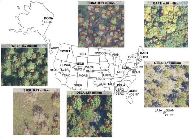
Locations of 37 NEON sites included in the NEON crowns data set and examples of tree predictions shown with RGB imagery for six sites.
Clockwise from bottom right: (1) OSBS: Ordway-Swisher Biological Station, Florida (2) DELA: Dead Lake, Alabama, (3) SJER: San Joaquin Experimental Range, California, (4) WREF: Wind River Experimental Forest, Washington, (5) BONA: Caribou Creek, Alaska and (6) BART: Bartlett Experimental Forest, New Hampshire. Each predicted crown is associated with the spatial position, crown area, maximum height estimates from co-registered LiDAR data, and a predicted confidence score.
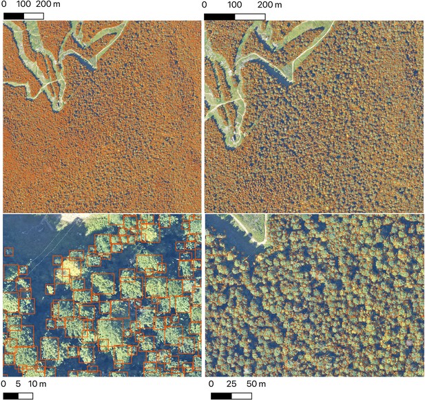
The Neon crowns data set provides individual-level tree predictions at broad scales.
An example from Bartlett Forest, NH shows the ability to continuously zoom from landscape level to stand level views. A single 1 km tile is shown. NEON sites tend to have between 100 and 400 tiles in the full airborne footprint.
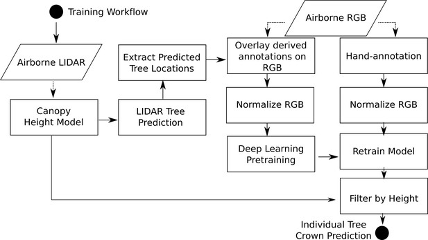
Workflow diagram adapted from Weinstein et al., 2020c.
The workflow for model training and development are identical to Weinstein et al., 2020c with the exception of extracting heights from the canopy height model for each bounding box prediction.
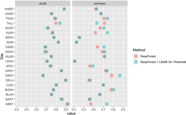
Precision and recall scores for the algorithm used to create the NEON crowns data set (red points), as well as the DeepForest model from Weinstein et al., 2020a (blue points).
Evaluation is performed on 207 image-annotated images (6926 trees) in the NEONTreeEvaluation data set (https://github.com/weecology/NeonTreeEvaluation). The small drop in recall in the LiDAR thresholding is due to the sparse nature of the LiDAR cloud which can occasionally miss valid trees over 3 m. Overlapping points show areas without change between the methods.
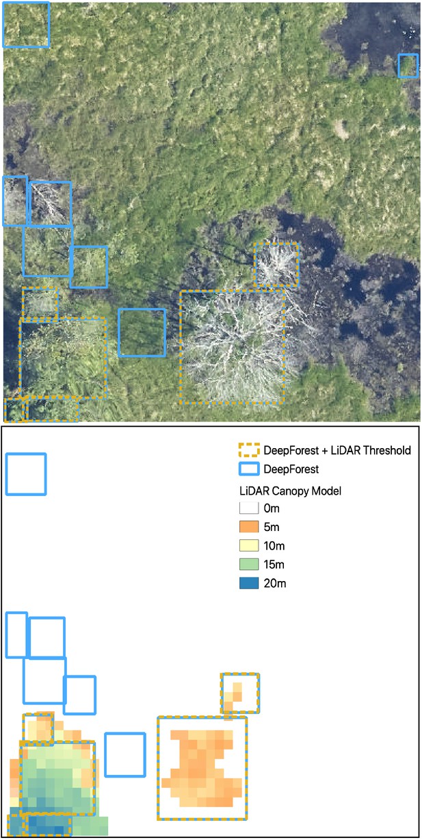
Illustration of the LiDAR threshold for minimum predicted tree height.
To utilize LiDAR information in the post-processing step we decided on a single 3 m threshold to eliminate erroneous predictions of shrubs and bare ground as trees. This occurred in open sites, especially at the edges of marshy habitat, where the test of bare ground can appear similar to tree crowns due to low lying vegetation with sharp boundaries against water features. The figure demonstrates the LiDAR threshold for minimum predicted tree height using NEON plot ID OSBS_023 from Ordway Swisher Biological Station, Florida. Using the DeepForest algorithm (Weinstein et al., 2020c), in blue, several boxes were removed based on no LiDAR returns above 3 m (dotted orange). This step was key in open-ground areas in which the algorithm can confuse short vegetation with standing trees.
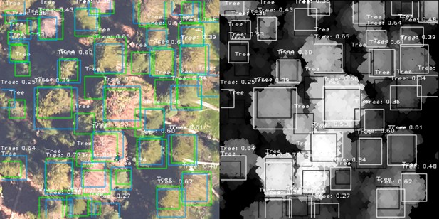
Illustration and discussion of attempts to incorporate LiDAR into DeepForest algorithm.
During the training of the DeepForest model, we experimented with many approaches to include multiple sources of RGB and LiDAR information on tree presence and crown shape. LiDAR data provides information on canopy height and is therefore commonly used as the primary data source for crown delineation. We attempted to incorporate LiDAR directly into DeepForest by using NEON’s canopy height model (CHM) as raster image alongside the three band RGB image to create a four-band stack. While this seems straightforward it changes the model weights so that they are no longer related to the three band pretraining using the ImageNet data set. This means that the neural network must be instantiated with random weights. This requires the network to learn basic feature representations of colors, shapes, and lines rather than inheriting this kind of information from the pretrained model. Given the paucity of labeled data, this leads to overfitting of the network. For example, when tested on the 18 hand annotated plots for the TEAK NEON site, the RGB-only mAP score was 0.529, whereas the combined RGB + CHM score was 0.389. Informal testing on flat-topped canopies in forests such as MLBS and LENO showed a disconnect between the LiDAR prediction and RGB predictions. In general, the CHM + RGB stack did not offer meaningful improvements in predictions and is therefore not currently included in the model. This may be due in part to the point densities of much of NEON’s LiDAR data. Most LiDAR based methods are evaluated on LiDAR data from a single forest type with point densities ranging from ~15 pts/m (e.g., Duncanson and Dubayah, 2018) to over 100 pts/m (e.g., Aubry-Kientz et al., 2019). In contrast, NEON’s current continental airborne LiDAR program produces ~6 pts/m and these densities can be highly variable, with large areas containing less than 4 pts/m. This tradeoff is needed to cover the much larger areas than previous studies.
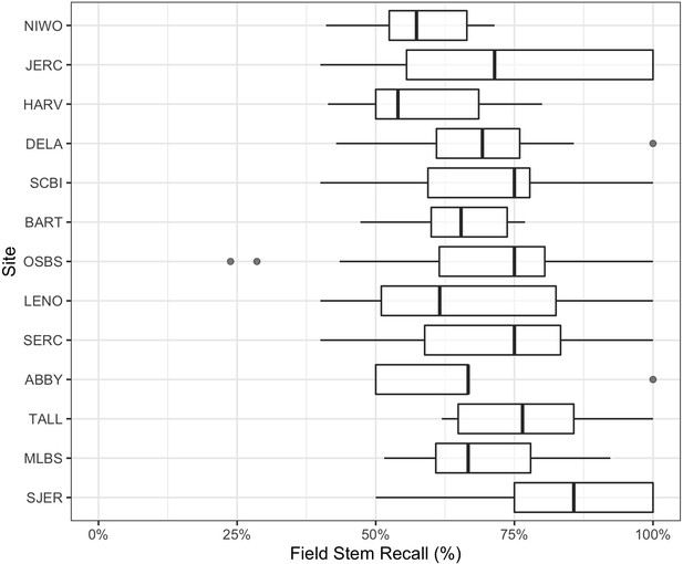
Overstory stem recall rate for NEON sites with available field data.
Each data point is the recall rate for a field-collected plot. NEON plots are either 40m × 40 m ‘tower’ plots with two 20 × 20 m subplots, or a single 20 m × 20 m ‘distributed’ plot. See NEON sampling protocols for details. For site abbreviations see Appendix 1 for complete table.
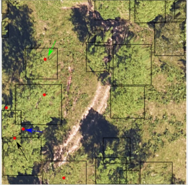
Description of workflow for filtering data to only include live trees likely to be visible in the canopy.
Raw NEON tree stem data was processed from the NEON data portal to provide a data set to compare image derived heights to field measured heights. The following filters were applied to the raw NEON field data (ID: DP1.10098.001) after download. A reference tree must have (1) valid spatial coordinates, (2) a unique height measurement per sampling period; individuals double recorded but with different heights were discarded, (3) height measurements in more than 1 year to verify height measurement, (4) changes in between-year field heights of less than 6 m, (5) a classification as alive, (6) a minimum height of 3 m to match the threshold in the remote sensing workflow, and (7) be at least within 5 m of the canopy as measured by the LiDAR height model extracted at the stem location. This was used to prevent matching with understory trees in the event that overstory trees were eliminated due to failing in one of the above conditions, or not sampled by NEON. To match trees in the field and the NEON Crowns data set, we took the closest height when two predictions and field stems overlapped. We also dropped CLBJ since only three points met these criteria. All other NEON sites did not have any data that met these criteria. In this figure we show stem recall for evaluation plot JERC_048 from Jones Ecological Resource Center, Georgia. Predicted tree bounding boxes in black. Filtered NEON field stems (see above for filtering criteria) in red. The green arrow shows the simplest scenario, a single prediction unambiguously overlaps a single collected stem. The black arrow shows a moderately challenging scenario in which a visually unambiguous crown only barely matches the field collected stem. This could occur due to (1) the stem growing at an angle leading to a spatial mismatch between crown and stem, (2) spatial error in measuring the crown location, and (3) spatial error in the georeferencing of the RGB image. The blue arrow shows a stem point that does not overlap with a prediction crown. We have written the stem recall evaluation to be conservative, allowing no tolerance for points outside of the prediction box. Therefore, the stem recall for this image was 4/6 = 66.66%, which we believe is a conservative representation of the performance of the algorithm given the uncertainty in the field data and matching process.
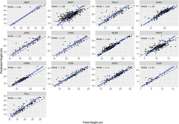
Comparison of field and remote sensing measurements of tree heights for 11 sites in the National Ecological Observatory Network.
Each point is an individual tree. See text and Figure 5—figure supplement 1 for selection criteria and matching scheme for the field data. The root mean squared error (RMSE) of a mixed-effects model with a site level random effect is 1.73 m.
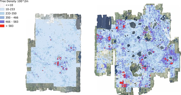
Tree density maps for Teakettle Canyon, California (left) and Ordway Swisher Biological Station, Florida (right).
For each 100 m2 pixel, the total number of predicted crowns were counted.

Illustrations of data quality challenges in remote sensing data.
With over 7000 1 km2 tiles, it is not possible to do a systematic check of data and predicted crowns. However, there are several general issues that we have encountered that are worth noting. Data quality errors include incomplete site coverage, image artifacts due to georectification, errors in orthomosaic stitching, and lighting changes among data collection events. (Top left) Patchy coverage at the site level can prevent broad scale analysis with large gaps in RGB data availability (NEON site GRSM). (Top right) RGB artifacts at the edge of images stem from the challenge of georectification of the RGB and LiDAR tiles leading to swirling in the RGB pixels (NEON site OSBS). (Bottom left) Seams in the flight-lines in the RGB images lead to gaps in local predictions (NEON site DELA). (Bottom right) Changes in illumination among data acquisition collections lead to stark changes in pixel values.
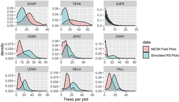
Comparison of tree counts between the field-collected NEON plots and the predicted plots from the data set.
For the remote sensing data, 10,000 simulated 40 m2 plots were calculated for each site for the full AOP footprint for each year. To mimic NEON sampling, two quadrants were randomly sampled in each simulated plot. No plots on water, bare ground, or herbaceous land classes were included in the comparison. We selected three sites from three NEON domains to show a sample of sites across the continental United States. Both distributed and tower NEON plots were used for these analyses.
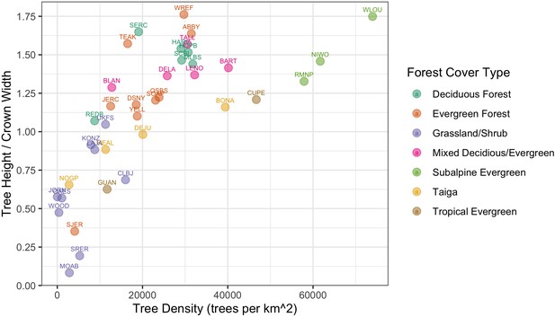
Individual crown attributes for predictions made at each NEON site.
For site abbreviations see Appendix 1. Crown area is calculated by multiplying the width and height of the predicted crown bounding box. Crown height is the 99th quantile of the LiDAR returns that fall inside the predicted crown bounding box. Sites are colored by the dominant forest type to illustrate the general macroecological relationship among sites in similar biomes.


