Influence of sensory modality and control dynamics on human path integration
- Center for Neural Science, New York University, United States
- Center for Theoretical Neuroscience, Columbia University, United States
- Ernst Strüngmann Institute for Neuroscience, Germany
- Department of Electrical and Computer Engineering, Rice University, United States
- Department of Neuroscience, Baylor College of Medicine, United States
- Center for Neuroscience and Artificial Intelligence, Baylor College of Medicine, United States
- Tandon School of Engineering, New York University, United States
Figures
Figure 1 with 3 supplements
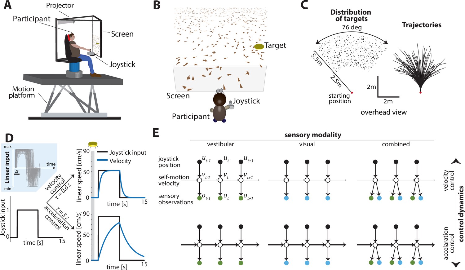
Experimental design.
(A) Experimental setup. Participants sit on a six-degrees-of-freedom motion platform with a coupled rotator that allowed unlimited yaw displacements. Visual stimuli were back-projected on a screen (see Materials and methods). The joystick participants used to navigate in the virtual world is mounted in front of the participants’ midline. (B) Schematic view of the experimental virtual environment. Participants use a joystick to navigate to a cued target (yellow disc) using optic-flow cues generated by ground plane elements (brown triangles; visual and combined conditions only). The ground plane elements appeared transiently at random orientations to ensure they cannot serve as spatial or angular landmarks. (C) Left: Overhead view of the spatial distribution of target positions across trials. Red dot shows the starting position of the participant. Positions were uniformly distributed within the participant’s field of view. Right: Movement trajectories of one participant during a representative subset of trials. Starting location is denoted by the red dot. (D) Control dynamics. Inset: Linear joystick input from a subset of trials in the visual condition of an example participant. Left: Simulated maximum pulse joystick input (max joystick input = 1) (see also Figure 1—figure supplement 3). This input is lowpass filtered to mimic the existence of inertia. The time constant of the filter varies across trials (time constant τ). In our framework, maximum velocity also varies according to the time constant τ of each trial to ensure comparable travel times across trials (see Materials and methods – Control Dynamics). Right: The same joystick input (scaled by the corresponding maximum velocity for each τ) produces different velocity profiles for different time constants (τ = 0.6 s corresponds to velocity control; τ = 3 s corresponds to acceleration control; τ values varied randomly along a continuum across trials, see Materials and methods). Also depicted is the brief cueing period of the target at the beginning of the trial (gray zone, 1 s long). (E) Markov decision process governing self-motion sensation (Materials and methods – Equation 1a). , , and denote joystick input, movement velocity, and sensory observations, respectively, and subscripts denote time indices. Note that due to the 2D nature of the task, these variables are all vector-valued, but we depict them as scalars for the purpose of illustration. By varying the time constant, we manipulated the control dynamics (i.e., the degree to which the current velocity carried over to the future, indicated by the thickness of the horizontal lines) along a continuum such that the joystick position primarily determined either the participant’s velocity (top; thin lines) or acceleration (bottom; thick lines) (compare with (D) top and bottom, respectively). Sensory observations were available in the form of vestibular (left), optic flow (middle), or both (right).
Figure 1—figure supplement 1
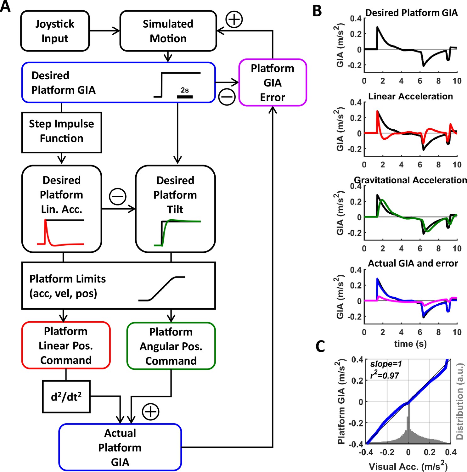
Motion Cueing framework.
(A) Flow diagram of motion-cueing (MC) algorithm.
The participant pilots themselves in a simulated environment using a joystick. The MC algorithm aims at controlling a platform such that the sum of inertial and gravitational acceleration experienced when sitting on the platform (desired platform gravito-inertial acceleration [GIA], blue; the curve illustrates an example profile consisting of a single rectangular waveform) matches the linear acceleration experienced in the simulated virtual environment. ‘Desired’ refers to the fact that the motion platform may not be able to match this acceleration exactly. The desired GIA is fed through a step impulse function to compute the desired linear acceleration of the platform. The difference between the desired linear acceleration and GIA is used to compute the desired platform tilt. The desired platform motion (linear and tilt motion) are passed through a controller that restricts its motion to the actuator’s limits (in terms of linear and angular acceleration, velocity, and position). The two actuator output commands are sent to the platform and are also used to compute the actuator GIA which is actually rendered by the platform. To ensure that the inertial motion produced by the platform matches the motion in the simulated environment, the actuator GIA is compared to the desired linear acceleration to compute an actuator GIA error feedback signal, which updates the simulated motion. (B) Acceleration profile of an actual trial. The first panel shows the desired GIA of the participant for that trial. The second and third panels show the desired linear acceleration (red) and desired tilt acceleration (green), respectively. The fourth panel shows the final GIA achieved (blue) and the GIA error (magenta). (C) Correspondence between visual acceleration and platform GIA (blue), measured independently from the MC algorithm using an inertial measurement unit mounted next to the participant’s head. There is an almost perfect match between the two. The gray histogram indicates the range of acceleration experienced by the participant.
Figure 1—figure supplement 2
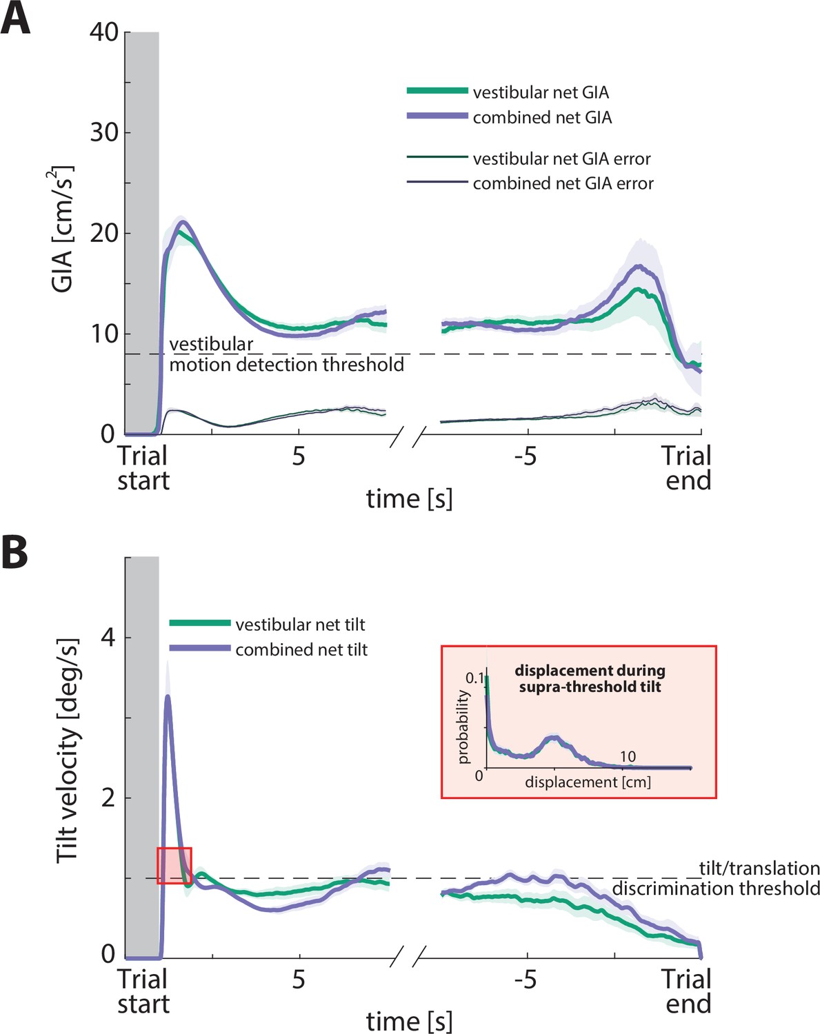
Verification of Motion Cueing output.
(A) Net gravito-inertial acceleration (GIA; thick lines) and net GIA error (thin lines) aligned to start and end of trial, for the vestibular and combined conditions across participants (average across trials over all time constants).
The dashed line represents a conservative choice of the vestibular motion detection threshold according to the relevant literature (8 cm/s2; Kingma, 2005; MacNeilage et al., 2010; Zupan and Merfeld, 2008). Gray region represents the target presentation period. Shaded regions denote ±1 SEM. (B) Net tilt velocity aligned to start and end of trial, for the vestibular and combined conditions across participants. Dashed line represents the estimated tilt/translation discrimination threshold of 1 deg/s: although tilt/translation discrimination thresholds have not been explicitly studied, we can use the rotation sensation thresholds of the semicircular canals to estimate what that threshold would be. Since it is the rotation velocity that tells a participant that they are tilting and not translating, we propose that the tilt/translation discrimination threshold is at least the same as the rotation sensation threshold (if not larger; Lim et al., 2017; MacNeilage et al., 2010). Shaded regions represent ±1 SEM across participants. Inset shows the probability distribution of displacements during the suprathreshold tilt period after trial onset (~0.6 s). Although the tilt can be perceived by the participants during trial onset, the displacement during that period does not exceed 10 cm and could potentially not contribute significantly to steering errors, for three reasons: (a) the displacement during that period is negligible, (b) tilt velocity is kept below the perceptual threshold for the remainder of the trajectory, (c) GIA is always above the motion detection threshold of the vestibular system. However, since the initial tilt could be perceived (as it briefly exceeded the canal detection threshold), this might alter the perceived orientation of the participants. In turn, this could influence the extent to which vestibular cues would be used as input to the path integration system (see Discussion ‘Limitations and future directions’ for further discussion). Thus, perceived tilt might be used as an indicator of trial onset, but it cannot contribute to path integration for three reasons: (a) the displacement during that period is negligible, (b) tilt velocity is kept below the perceptual threshold for the remainder of the trajectory, (c) GIA is always above the motion detection threshold of the vestibular system.
Figure 1—figure supplement 3
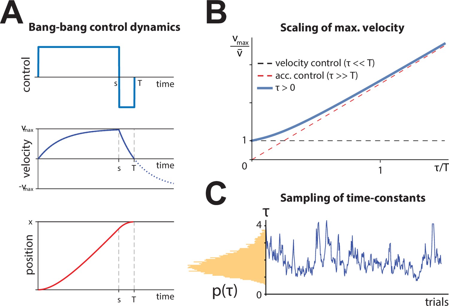
Control dynamics framework.
(A) Example dynamics for bang-bang control.
Position, velocity, and controls are shown. Control switches at time s and ends at time T. (B) Maximal velocity (blue) needed for bang-bang control to produce a desired average velocity , as a function of the fraction of trial duration given by the time constant, . When the time constant is a small fraction of the trial (velocity control), the max velocity equals the average velocity (orange line). When the time constant is much longer than a trial (acceleration control), the maximum velocity grows as (green), although this speed is never approached since braking begins before the velocity approaches equilibrium. (C) Example dynamics for control behavior. Left: Log-normal distribution of control time constants (see also Figure 3—figure supplement 1A). Right: Example random walk in space.
Figure 2 with 2 supplements
Effect of sensory modality on participants' responses.
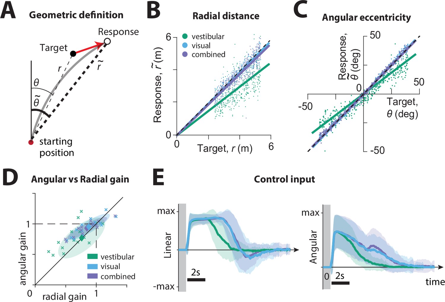
(A) Geometric definition of analysis variables.
The gray solid line indicates an example trajectory. The target and response distance and angle relative to the starting position of the participant are given by (thin lines) and (thick lines), respectively. (B C) Example participant: Comparison of the radial distance of an example participant’s response (final position) against the radial distance of the target (B), as well as the angular eccentricity of the participant’s response vs. target angle (C), across all trials for one participant, colored according to the sensory condition (green: vestibular, cyan: visual, purple: combined visual and vestibular; Figure 2—source data 1). Radial and angular response gains were defined as the slope of the corresponding regressions. Black dashed lines show unity slope, and the solid lines represent slopes of the regression fits (intercept set to 0). (D) All participants: Radial and angular gains in each sensory condition plotted for each individual participant (Figure 2—source data 2). Ellipses show 68% confidence intervals of the distribution of data points for the corresponding sensory condition. Diamonds (centers of the ellipses) represent the mean radial and angular response gains across participants. Dashed lines indicate unbiased radial or angular position responses. Solid diagonal line has unit slope. (E) Magnitudes of radial and angular components of control inputs across sensory conditions for an example participant. Shaded regions represent ±1 standard deviation across trials. The gray zone corresponds to the target presentation period.
-
Figure 2—source data 1
Radial and angular responses.
- https://cdn.elifesciences.org/articles/63405/elife-63405-fig2-data1-v2.zip
-
Figure 2—source data 2
Response gains.
- https://cdn.elifesciences.org/articles/63405/elife-63405-fig2-data2-v2.zip
Figure 2—figure supplement 1
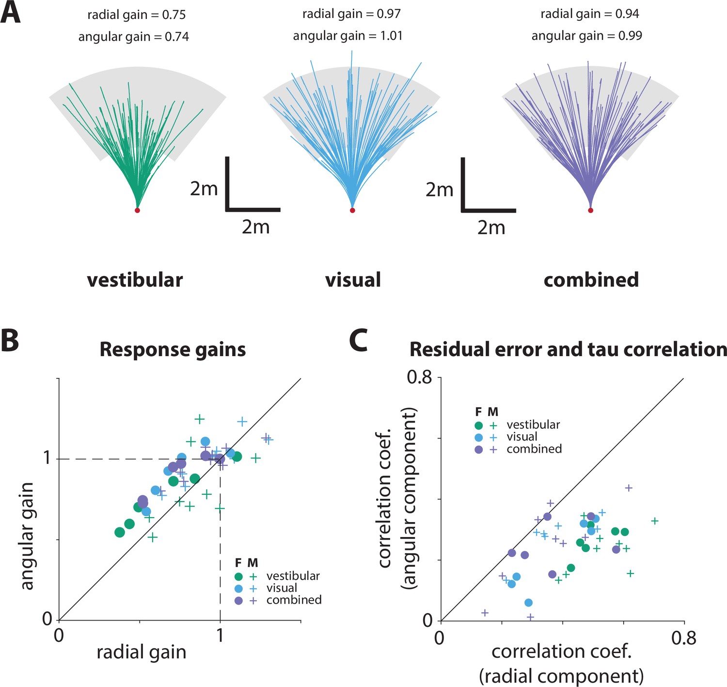
Trajectories in all conditions and sex differences in performance.
(A) Random subset of trajectories of an example participant under each sensory condition. The corresponding radial and angular response gains are indicated for each condition (green: vestibular, cyan: visual, purple: combined). Gray region represents the target range. (B) Sex differences in participants’ performance: radial and angular gains (see Figure 2D) grouped based on sex (F: female, M: male; see legend; p-values of differences in response gains between male and female participants: Radial gain – vestibular: p = 0.17, visual: p = 0.09, combined: p = 0.09; angular gain – vestibular: p = 0.58, visual: p = 0.38, combined: p = 0.21; two-sample t-test). (C) Sex differences in participants’ performance: correlation coefficients between the time constant and the residual errors (radial and angular components; see Figure 3C) grouped based on sex. Specifically, the x and y axes represent the correlation values between the time constant and the radial and angular residual errors, respectively (p-values of differences in correlation coefficients between male and female participants: Radial – vestibular: p = 0.5, visual: p = 0.66, combined: p = 0.71; angular – vestibular: p = 0.51, visual: p = 0.97 combined: p = 0.82 two-sample t-test).
Figure 2—figure supplement 2
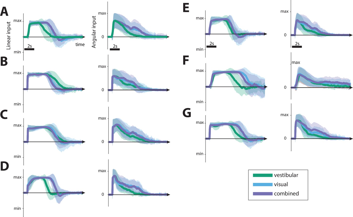
Joystick inputs.
(A–G) Linear (left) and angular (right) joystick input over time, for a subset of participants in all conditions (see legend; bottom right). The joystick control had shorter duration in the vestibular condition, reflecting our findings of the smaller response gains. Shaded regions represent ±1 standard deviation across trials.
Figure 3 with 2 supplements
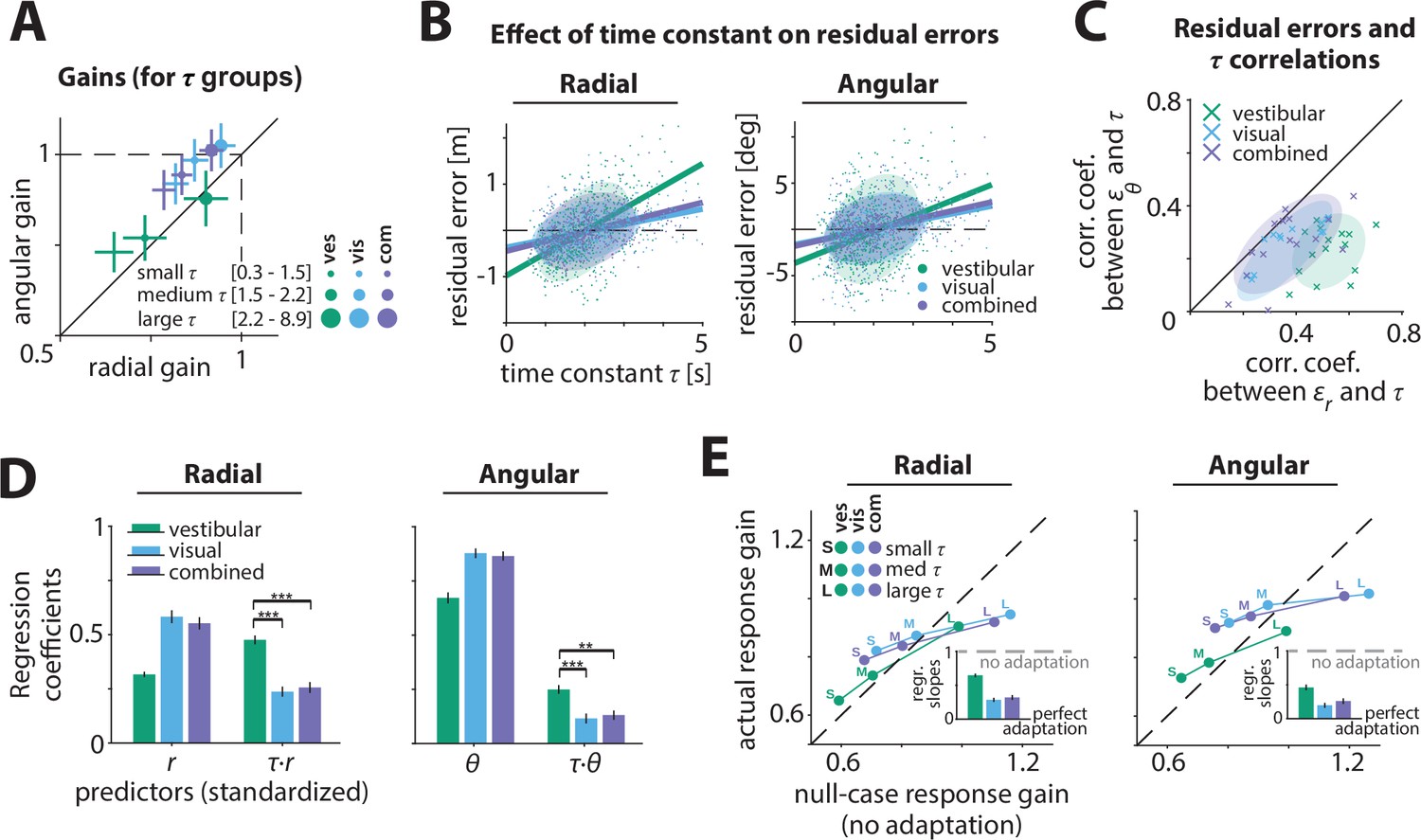
Effect of control dynamics on participants’ responses.
(A) Participant average of radial and angular response gains in each condition, with trials grouped into tertiles of increasing time constant τ. Error bars denote ±1 SEM. (B) Effect of time constant on radial (left) and angular (right) residual error, for an example participant (Figure 3—source data 1). Solid lines represent linear regression fits and ellipses the 68% confidence interval of the distribution for each sensory condition. Dashed lines denote zero residual error (i.e. stopping location matches mean response). (C) Correlations of radial () and angular () residual errors with the time constant for all participants. Ellipses indicate the 68% confidence intervals of the distribution of data points for each sensory condition. Solid diagonal line has unit slope. Across participants, radial correlations, which were larger for the vestibular condition, were greater than angular correlations (see also Appendix 2—table 2). (D) Linear regression coefficients for the prediction of participants’ response location (final position:, ; left and right, respectively) from initial target location (,) and the interaction between initial target location and the time constant (,) (all variables were standardized before regressing, see Materials and methods; Figure 3—source data 2). Asterisks denote statistical significance of the difference in coefficient values of the interaction terms across sensory conditions (paired t-test; *: p<0.05, **: p<0.01, ***: p<0.001; see main text). Error bars denote ±1 SEM. Note a qualitative agreement between the terms that included target location only and the gains calculated with the simple linear regression model (Figure 2B). (E) Comparison of actual and null-case (no adaptation) response gains, for radial (top) and angular (bottom) components, respectively (average across participants). Dashed lines represent unity lines, that is, actual response gain corresponds to no adaptation. Inset: Regression slopes between actual and null-case response gains. A slope of 0 or 1 corresponds to perfect or no adaptation (gray dashed lines), respectively. Error bars denote ±1 SEM.
-
Figure 3—source data 1
Residual errors.
- https://cdn.elifesciences.org/articles/63405/elife-63405-fig3-data1-v2.zip
-
Figure 3—source data 2
Regression coefficients between time constant and residual errors.
- https://cdn.elifesciences.org/articles/63405/elife-63405-fig3-data2-v2.zip
Figure 3—figure supplement 1
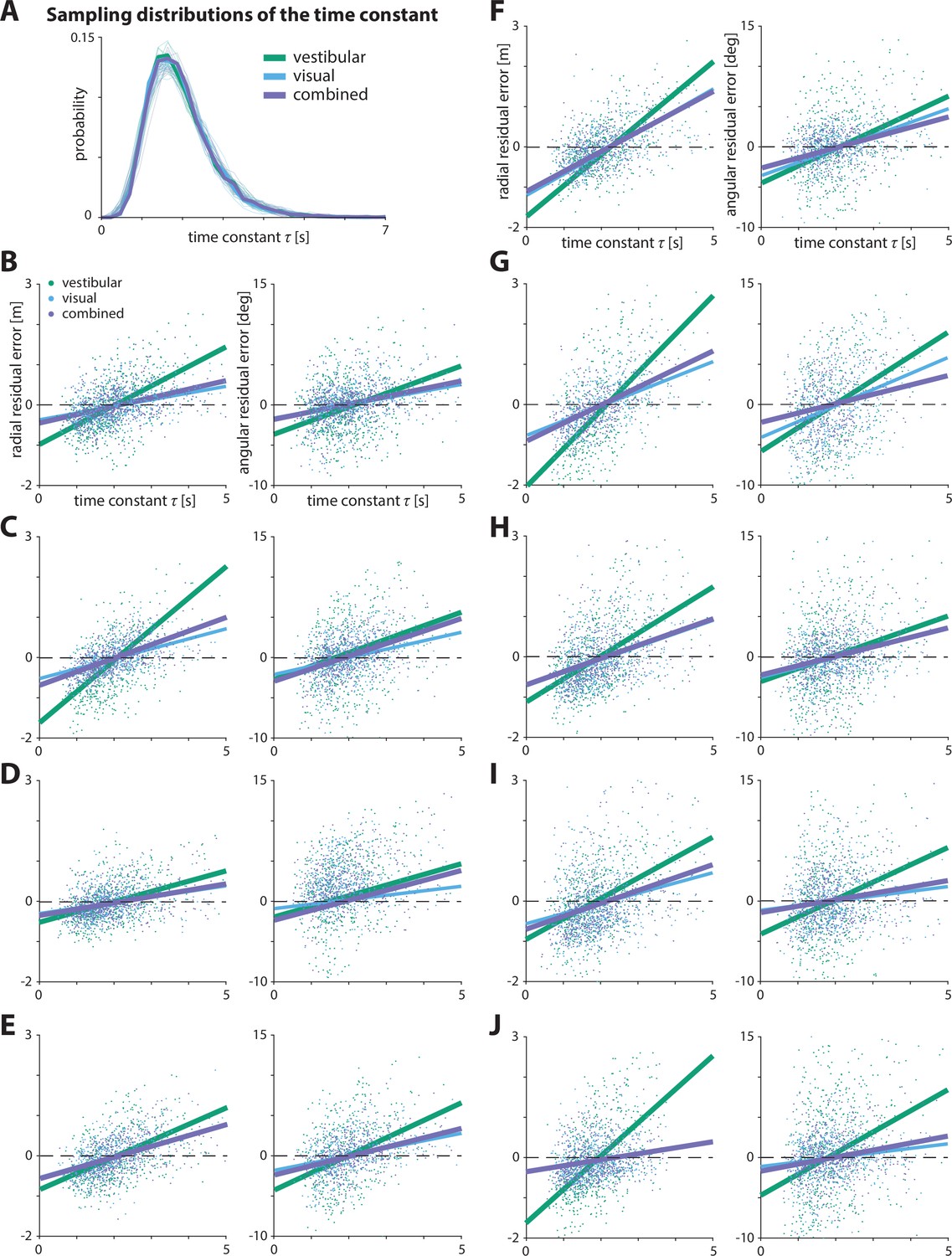
Effect of time constant on residual errors.
(A) Sampling distributions of the time constant for all three sensory conditions across participants.
The sampling distribution both across participants and across conditions is almost identical.
Transparent lines and thick lines represent the individual sampling distributions of participants and their mean, respectively. (B–J) Effect of the time constant on radial (left) and angular (right) residual error, for a large subset of participants.Solid lines represent linear regression fits (see Appendix 2—table 3 for individual regression coefficient values). Dashed lines denote zero residual error (i.e. stopping location matches mean response).
Figure 3—figure supplement 2
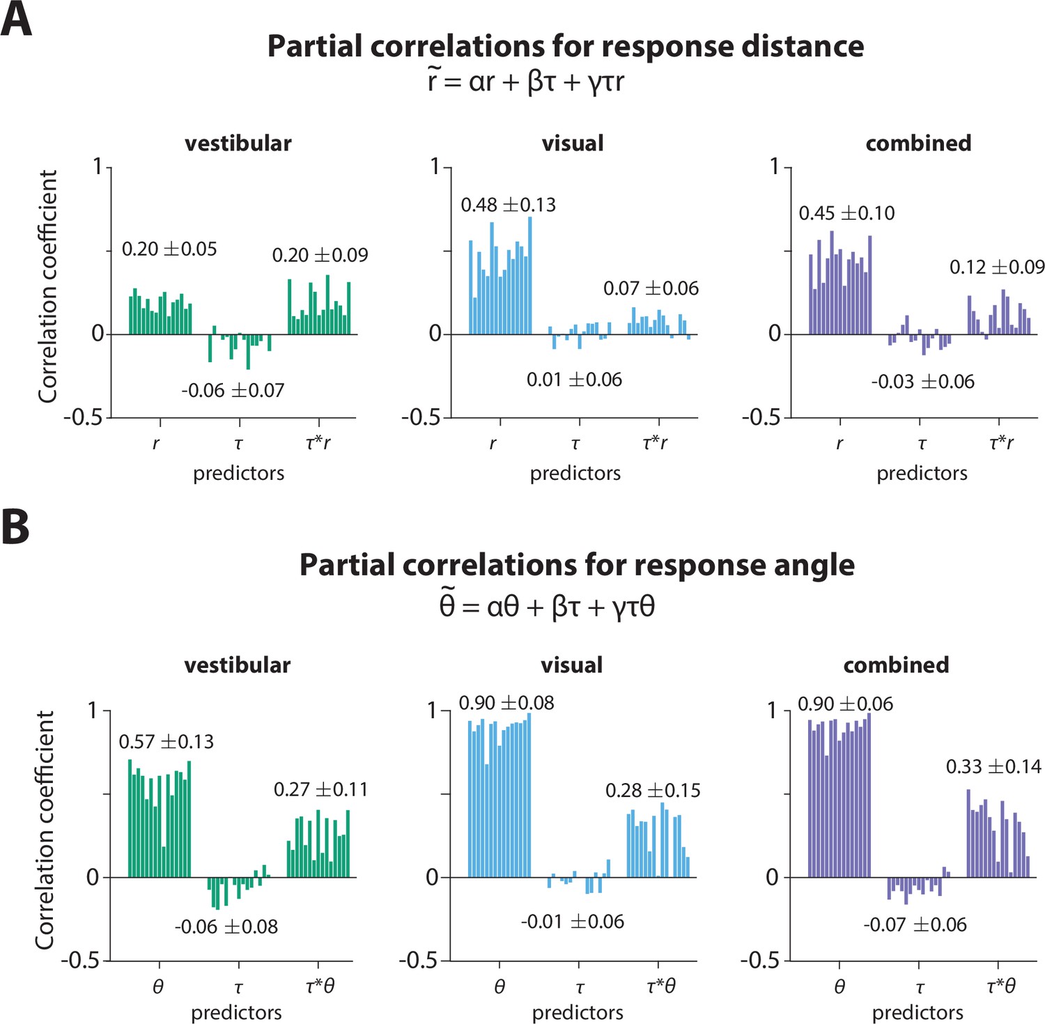
Partial correlation analysis.
(A) Partial correlation coefficients for prediction of stopping distance (relative to starting position) from initial target distance (), τ, and the interaction of the two (), for all participants across sensory conditions.
Values at each bar group represent the average coefficient value across participants ±1 standard deviation. The contribution of the τ-only term was considered insignificant across all conditions. The simplified version of this model would be: , which implies that the radial gain is τ-dependent. (B) Partial correlation coefficients for prediction of stopping angle (relative to starting position) from initial target angle (), τ, and the interaction of the two (), for all participants across sensory conditions. Values at each bar group represent the average coefficient value across participants ±1 standard deviation. In agreement with the findings for the response distance, the contribution of the τ-only term was considered insignificant across all conditions. The simplified version of this model would be: , which implies that the angular gain is also τ-dependent.
Figure 4
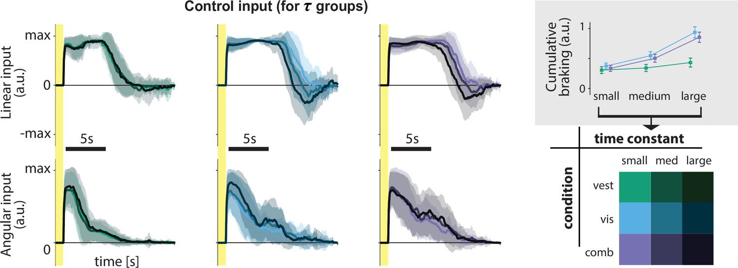
Linear and angular control inputs for each condition grouped based on the time constant (see legend; bottom right), for an example participant.
Shaded regions represent ±1 standard deviation across trials. Yellow zones denote target presentation period. Inset: Cumulative braking (i.e. absolute sum of negative linear input) for each condition across time constant groups. Braking was averaged across trials. Error bars denote ±1 SEM across participants.
Figure 5 with 2 supplements
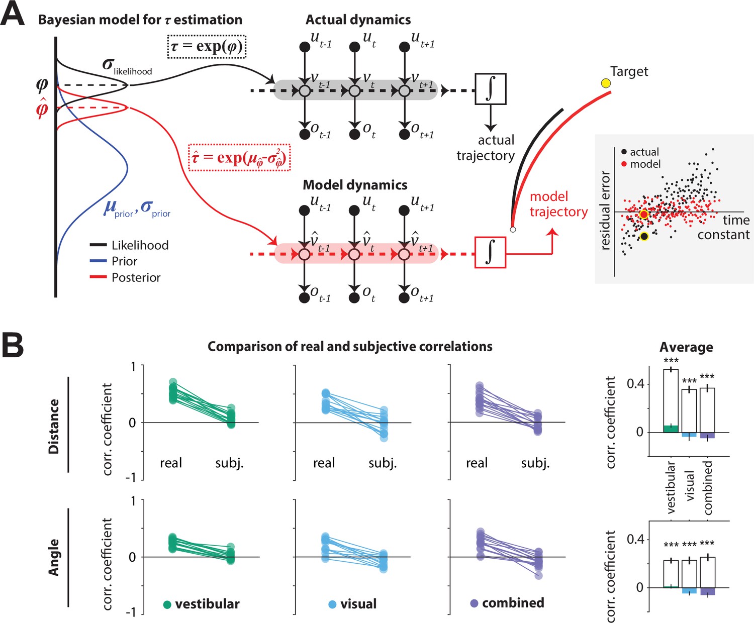
Bayesian model framework and correlations between the time constant and model-implied residual errors.
(A)Left: Illustration of the Bayesian estimator model. We fit two parameters: the ratio λ of standard deviations of prior and likelihood () and the mean of the prior of the normally distributed variable (black dotted box). Likelihood function is centered on the log-transformation of the actual τ, (black dashed line). The time constant estimate corresponded to the median of the posterior distribution over , which corresponds to the median over , (red dotted box;red dashed line; see Materials and methods). Middle: Control dynamics implied by the actual time constant (top; gray shade) and the estimated time constant (bottom; red shade). , , and denote joystick input, movement velocity, and sensory observations, respectively, and subscripts denote time indices. denotes the inferred velocity implied by the model. Misestimation of the time constant leads to erroneous velocity estimates about self-motion which result in biased position beliefs. Right: Illustration of the actual (black) and believed (red) trajectories produced by integrating (box) the actual velocity and the estimated velocity , respectively. White and yellow dots denote the starting and target position, respectively. Inset: Illustration of correlated (black dots) and uncorrelated (red dots) residual errors with the time constant for actual and model-implied responses (simulated data). For simplicity, we depict residual errors as one-dimensional and assume unbiased responses (response gain of 1). Blown-up dots with yellow halo correspond to the actual and model-implied trajectories of the right panel. Solid black horizontal line corresponds to zero residual error (i.e. stop on target location). (B) Comparison of correlations between real and subjective residual errors with τ (Figure 5—source data 1). On the right, participant averages of these correlations are shown. Colored bars: ‘Subjective’ correlations, open bars: Actual correlations. Error bars denote ±1 SEM across participants. Asterisks denote the level of statistical significance of differences between real and subjective correlations (*: p<0.05, **: p<0.01, ***: p<0.001).
-
Figure 5—source data 1
correlations between time constant and model-implied residual errors.
- https://cdn.elifesciences.org/articles/63405/elife-63405-fig5-data1-v2.zip
Figure 5—figure supplement 1
Testing model assumptions.
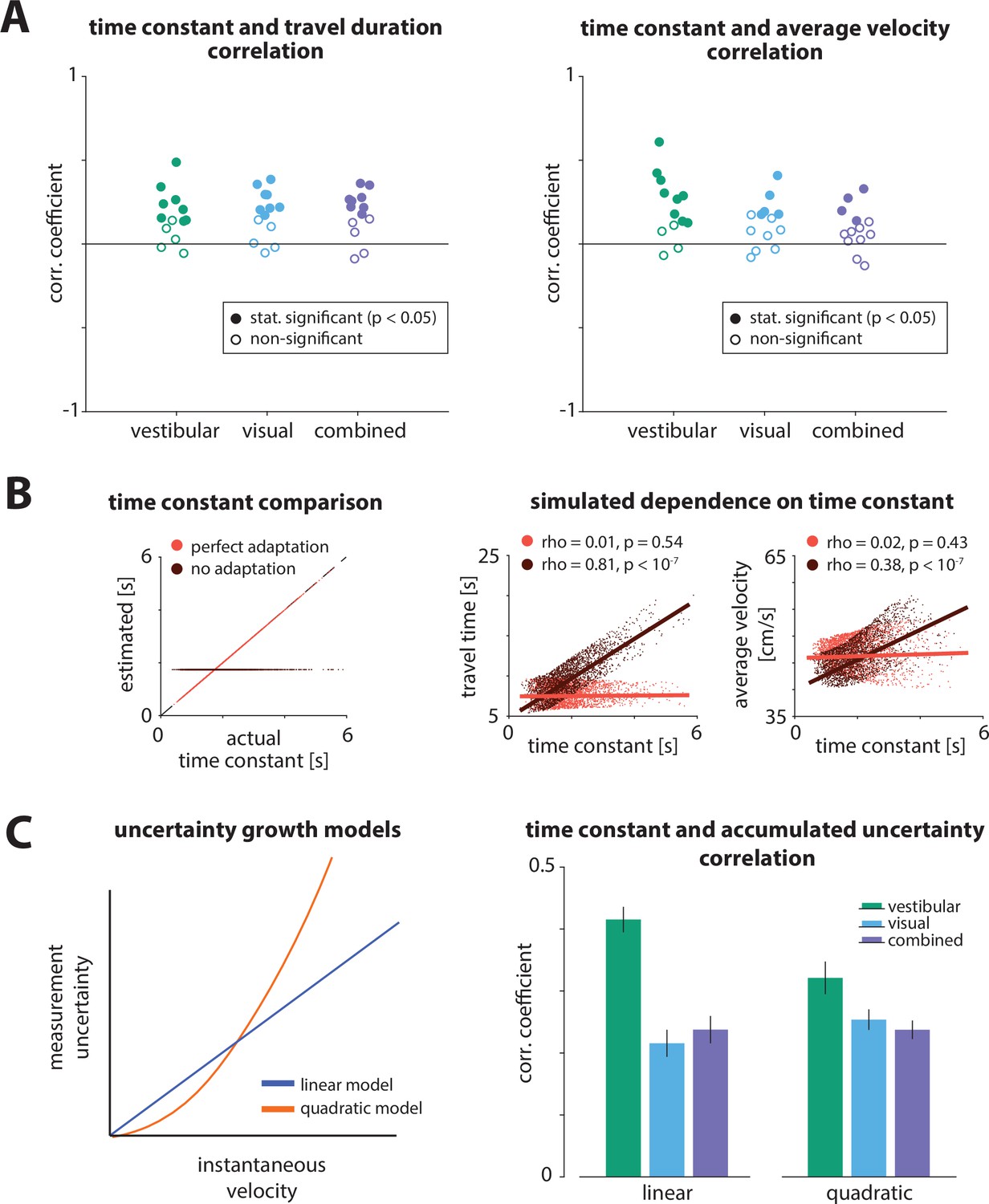
(A) Correlation coefficients between the time constant and travel duration (left) or average travel velocity (right) across trials for all participants.
Colors of circles indicate the sensory condition (green: vestibular, cyan: visual, purple: combined). Open and filled circles denote statistical significance according to the legend. (B) Dependence of travel duration (top right) and average velocity (bottom right) on the time constant for perfect or no estimation/adaptation to the dynamics (left), for a simulated bang-bang controller. Correlation coefficients and statistical significance are indicated in the legends of the corresponding panels. Solid lines represent linear regression fits. (C) Left: Uncertainty (variance) of instantaneous self-motion velocity estimation. Illustration of a linear (blue) and a quadratic (orange) model of velocity estimation uncertainty as a function of the instantaneous velocity magnitude. We wanted to test whether the effect of the time constant on performance could be attributed to differences in the accumulated uncertainty of the different velocity profiles. Right: Correlation between time constant and accumulated uncertainty for the linear and quadratic models. We found that the accumulated uncertainty is positively correlated with the time constant for both models (adding an intercept term to the models did not qualitatively change the results). This means that higher time constants yield larger uncertainty and, therefore, participants should undershoot more. However, this is the opposite of the observed effect of the time constant on the responses. Error bars denote ±1 SEM.
Figure 5—figure supplement 2
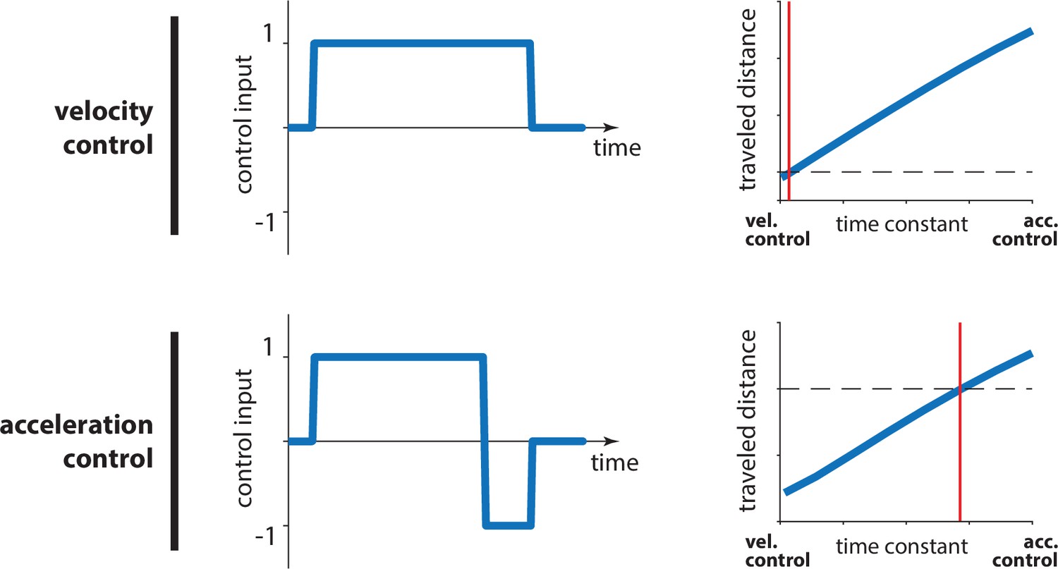
Changes in travel distance for a given control input under different control dynamics.
Whether in the domain of velocity (top) or acceleration control (bottom), a control input that is appropriate to reach a certain target distance (horizontal black dashed line) under only a certain time constant (red vertical line) will produce erroneous displacements under any other time constant (blue line). For smaller time constants, the intended distance will be undershot, whereas larger time constants will lead to overshooting. In other words, assuming that the red vertical line denotes the believed dynamics of a controller, a larger actual time constant (underestimation) will lead to overshooting (relative to the intended displacement; horizontal black dashed line). Inversely, overestimation of the time constant would lead to undershooting. Note that, for acceleration control, we chose a bang-bang controller such that we can demonstrate that this holds true whether there is braking at the end of the trial or not.
Figure 6
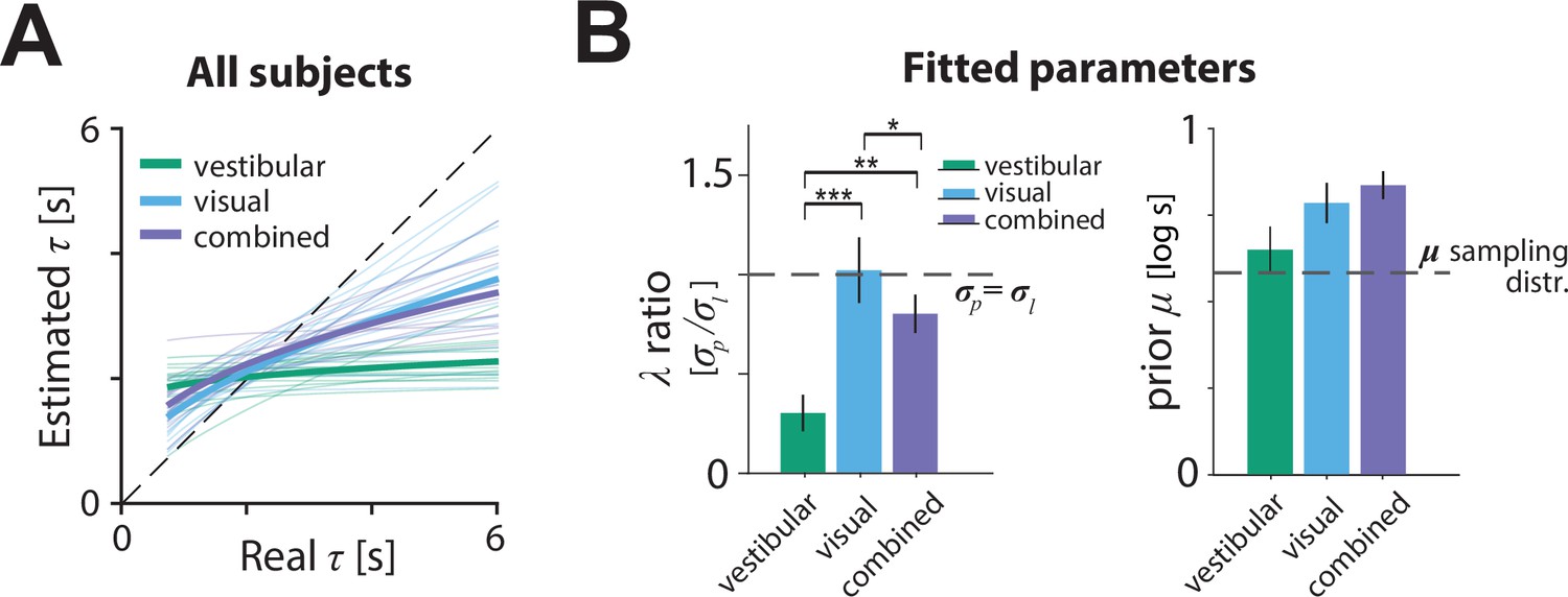
Model parameters.
(A) Relationship between the model-estimated and actual time constant across all participants in vestibular (green), visual (cyan), and combined (purple) conditions. Participant averages are superimposed (thick lines). Dashed line: unbiased estimation (Figure 6—source data 1). (B) Fitted model parameters: ratio of prior () over likelihood () standard deviation and mean () of prior. Error bars denote ±1 SEM. Dashed lines represent the corresponding values of the sampling distribution of , which is normal (see Materials and methods; Figure 6—source data 2). The prior distribution’s was comparable in the vestibular condition to the of the actual sampling distribution (sampling distribution : 0.58 – p-value of prior difference obtained by bootstrapping – vestibular: p = 0.014, visual: p =< 10–7; combined: p < 10–7). Asterisks denote the level of statistical significance of differences in the fitted parameters across conditions (*: p<0.05, **: p<0.01, ***: p<0.001).
-
Figure 6—source data 1
Real versus estimated time constants.
- https://cdn.elifesciences.org/articles/63405/elife-63405-fig6-data1-v2.zip
-
Figure 6—source data 2
Model parameters.
- https://cdn.elifesciences.org/articles/63405/elife-63405-fig6-data2-v2.zip
Figure 7 with 2 supplements
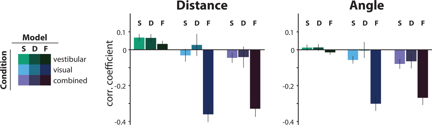
Comparison of the correlations between the actual τ and the subjective residual errors implied by three different τ-estimation models (Bayesian estimation with a static prior ([S], Bayesian estimation with a dynamic prior [D], fixed estimate [F]).
We tested the hypotheses that either the prior distribution should not be static or that the participants ignored changes in the control dynamics and navigated according to a fixed time constant across all trials (fixed τ estimate model; see Materials and methods). For this, we compared the correlations between the subjective residual error and the actual trial τ that each model produces. The dynamic prior model performs similarly to the static prior model in all conditions, indicating that a static prior is adequate in explaining our data (p-values of paired t-test between correlation coefficients of the two models: distance – vestibular: p = 0.96, visual: p = 0.19, combined: p = 0.91; angle – vestibular: p = 0.87, visual: p = 0.09, combined: p = 0.59). For visual and combined conditions, the fixed τ model not only fails to minimize the correlations but, in fact, strongly reverses it, for both distance (left) and angle (right). Since these correlations arise from the believed trajectories that the fixed τ model produces, this suggests that participants knowingly stop before their believed target location for higher time constants. Model performance was only comparable in the vestibular condition, where the average correlation of the fixed τ model (F) was contained within the 95% confidence intervals (CI) of the static prior Bayesian model (S), for both distance and angle (distance – F: mean Pearson’s correlation coefficient ρ = 0.03, S: 95% CI of Pearson’s correlation coefficient ρ = [–0.10 0.25]; angle – F: mean Pearson’s correlation coefficient ρ = –0.01, S: 95% CI of Pearson’s correlation coefficient ρ = [–0.12 0.15]). Error bars denote ±1 SEM.
Figure 7—figure supplement 1
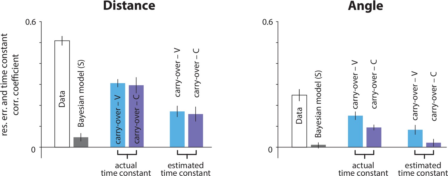
Correlation coefficients in the vestibular condition between the actual time constant and the subjective radial (left) and angular (right) residual errors, if participants carried over their τ estimate from the previous trial.
With sensory conditions interleaved and a common random walk of τ (see Materials and methods, Figure 1—figure supplement 3C), we searched for a trial-type history effect in the vestibular condition, due to participants’ poor τ estimation performance. Specifically, we asked whether participants in the vestibular condition would leverage from the correlation structure between recent time constants by carrying over their estimates from the previous visual or combined trials. We first compared the correlations from the actual data (open bars; same as Figures 3C and 5B) with those obtained when using the actual (middle bar couple) or estimated (right bar couple; estimates from the static prior Bayesian model) time constant from the previous visual (cyan bars) or combined (purple bars) trial to generate believed trajectories. Although correlations were significantly smaller for the carry-over models relative to the actual data (p<0.01) they nevertheless remained significant (p<10−5), thus, failing to explain away the effect (compare with gray bars: correlations implied by estimation in the current vestibular trial with the static prior Bayesian model). The carry-over strategy does not seem likely since it fails to explain away a large part of the correlation between the radial component of the subjective residual errors and the time constant (compare rightmost cyan/purple bars with gray bars; p-values of paired t-test between radial correlation coefficients – current vestibular vs. previous visual trial estimation: p=0.006, current vestibular vs. previous combined trial estimation: p=0.02; p-values of paired t-test between angular correlation coefficients – current vestibular vs. previous visual trial estimation: p=0.008, current vestibular vs. previous combined trial estimation: p = 0.71). Error bars denote ±1 SEM across participants.
Figure 7—figure supplement 2
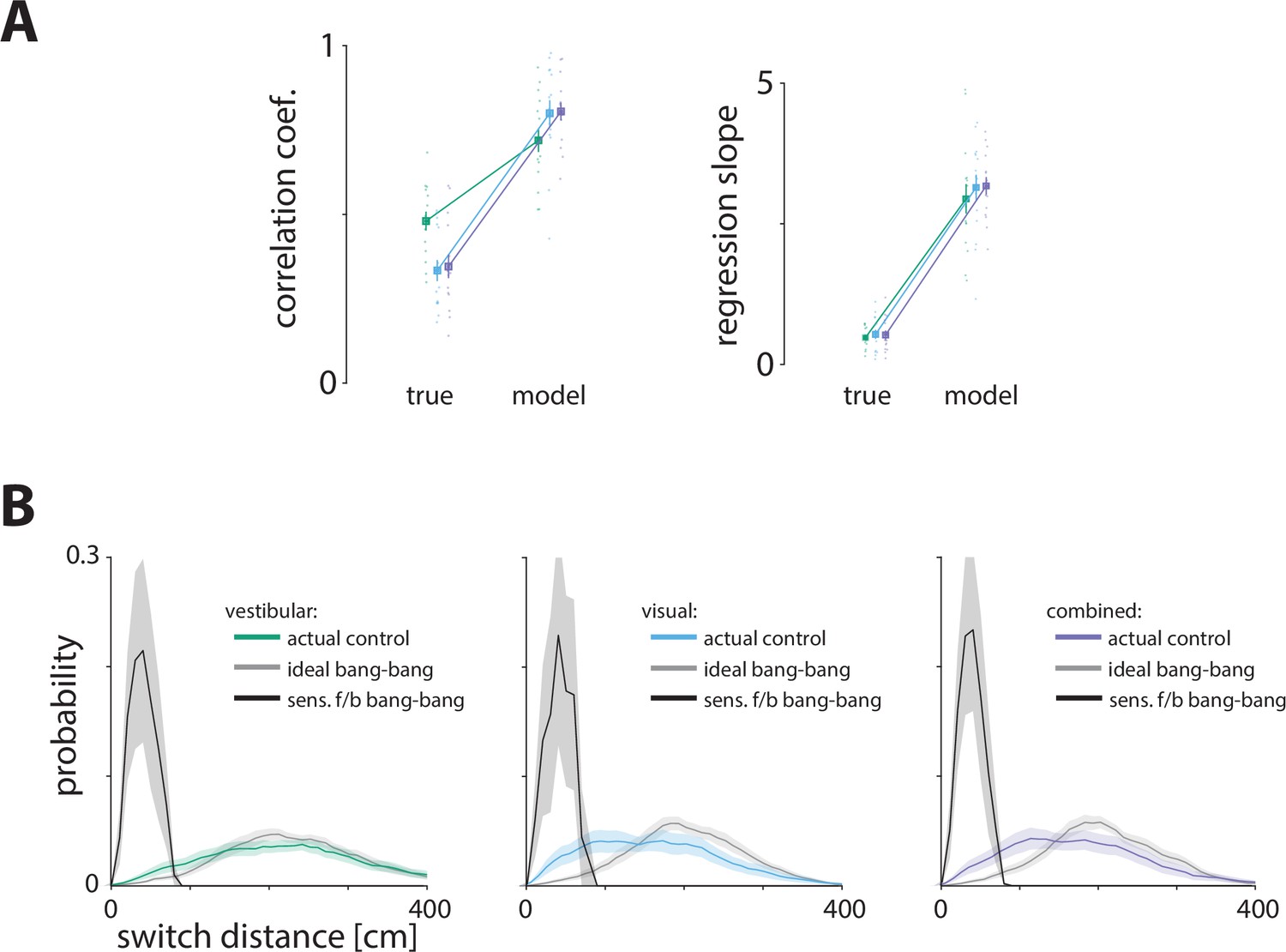
Comparing bayesian and feedback control models.
(A) We tested a sensory feedback control model, in which the controller uses bang-bang control and switches from forward to backward input at a constant and predetermined distance from the target position (corrected for the bias).
We fit the mean and standard deviation of the switch distance for each participant in each condition separately, by minimizing the distance of the actual from the model-predicted stopping locations (see Materials and methods). The correlations (left) and the regression slopes (right) between the model-predicted residual errors and the time constant were significantly higher than those found in our data (p-values of difference in correlations between true data and model obtained by paired t-test – vestibular: p = 10–5, visual: p = 10–6, combined: p = 10–7; p-values of difference regression slopes between true data and model obtained by paired t-test – vestibular: p = 10–7, visual: p = 10–8, combined: p = 10–9). Error bars represent ±1SEM across participants. (B) Probability distribution of bang-bang switch distance from target position (corrected for the bias). According to the sensory feedback control model, the probability distribution of switch distance should be very narrow since participants switch at a constant perceived distance from the target. If participants implemented this type of control (black lines), we would expect to see such a narrow distribution in the actual data. In all conditions, however, the switch distance distribution of the true data (colored lines) is wider and resembles what we expect to see if participants implemented optimal (ideal) bang-bang control (gray lines). Shaded regions represent ±1 SEM across participants.
Tables
Appendix 2—table 1
Average radial (top) and angular (bottom) behavioral response gains across participants, for groups of time constant τ magnitudes (mean ± SEM).
| Radial bias table | |||
|---|---|---|---|
| Vestibular | Visual | Combined | |
| τ: [0.34–1.53] | 0.649 ± 0.056 | 0.818 ± 0.057 | 0.786 ± 0.055 |
| τ: [1.53–2.16] | 0.733 ± 0.063 | 0.871 ± 0.059 | 0.836 ± 0.056 |
| τ: [2.16–8.89] | 0.902 ± 0.077 | 0.944 ± 0.061 | 0.917 ± 0.058 |
| Angular bias table | |||
| Vestibular | Visual | Combined | |
| τ: [0.34–1.53] | 0.731 ± 0.053 | 0.919 ± 0.036 | 0.902 ± 0.032 |
| τ: [1.53–2.16] | 0.770 ± 0.060 | 0.984 ± 0.038 | 0.944 ± 0.029 |
| τ: [2.16–8.89] | 0.878 ± 0.061 | 1.024 ± 0.040 | 1.012 ± 0.033 |
Appendix 2—table 2
Pearson’s correlation coefficient (r) and corresponding p-value (p) for radial (top) and angular (bottom) correlation between residual error and the time constant τ across participants.
Mean Pearson’s r ± SEM: radial component – vestibular: 0.52±0.02, visual: 0.36±0.03, combined: 0.37±0.03; angular component – vestibular: 0.23±0.02, visual: 0.23±0.03, combined: 0.26±0.03.
| Radial correlations | |||
|---|---|---|---|
| Vestibular | Visual | Combined | |
| Subject 1 | r = 0.585, p = 4.2·10–45 | r = 0.502, p = 1.2·10–37 | r = 0.617, p = 1.0·10–59 |
| Subject 2 | r = 0.622, p = 5.5·10–43 | r = 0.338, p = 7.4·10–12 | r = 0.377, p = 2.9·10–14 |
| Subject 3 | r = 0.433, p = 3.5·10–25 | r = 0.280, p = 2.7·10–11 | r = 0.374, p = 8.7·10–20 |
| Subject 4 | r = 0.492, p = 9.1·10–31 | r = 0.494, p = 3.1·10–31 | r = 0.350, p = 2.1·10–15 |
| Subject 5 | r = 0.411, p = 4.4·10–17 | r = 0.314, p = 3.4·10–10 | r = 0.360, p = 3.7·10–13 |
| Subject 6 | r = 0.601, p = 2.0·10–58 | r = 0.233, p = 1.2·10–08 | r = 0.233, p = 1.2·10–08 |
| Subject 7 | r = 0.606, p = 1.6·10–44 | r = 0.522, p = 1.5·10–31 | r = 0.474, p = 1.1·10–25 |
| Subject 8 | r = 0.477, p = 9.6·10–34 | r = 0.255, p = 5.7·10–10 | r = 0.294, p = 4.6·10–13 |
| Subject 9 | r = 0.478, p = 1.0·10–22 | r = 0.517, p = 7.9·10–27 | r = 0.523, p = 6.3·10–28 |
| Subject 10 | r = 0.573, p = 7.2·10–39 | r = 0.497, p = 4.7·10–28 | r = 0.576, p = 3.5·10–39 |
| Subject 11 | r = 0.375, p = 5.9·10–16 | r = 0.224, p = 2.1·10–06 | r = 0.144, p = 0.002 |
| Subject 12 | r = 0.522, p = 2.1·10–39 | r = 0.341, p = 1.3·10–16 | r = 0.319, p = 1.1·10–14 |
| Subject 13 | r = 0.512, p = 1.1·10–38 | r = 0.385, p = 1.4·10–21 | r = 0.401, p = 4.7·10–23 |
| Subject 14 | r = 0.461, p = 8.3·10–30 | r = 0.241, p = 1.3·10–08 | r = 0.276, p = 7.0·10–11 |
| Subject 15 | r = 0.703, p = 1.7·10–61 | r = 0.214, p = 1.1·10–05 | r = 0.213, p = 1.3·10–05 |
| Angular correlations | |||
| Vestibular | Visual | Combined | |
| Subject 1 | r = 0.254, p = 1.9·10–08 | r = 0.302, p = 1.8·10–13 | r = 0.437, p = 2.3·10–27 |
| Subject 2 | r = 0.156, p = 0.002 | r = 0.287, p = 8.6·10–09 | r = 0.270, p = 9.2·10–08 |
| Subject 3 | r = 0.301, p = 2.2·10–12 | r = 0.274, p = 7.3·10–11 | r = 0.351, p = 1.7·10–17 |
| Subject 4 | r = 0.315, p = 1.3·10–12 | r = 0.299, p = 1.7·10–11 | r = 0.343, p = 8.9·10–15 |
| Subject 5 | r = 0.153, p = 0.003 | r = 0.291, p = 6.7·10–09 | r = 0.387, p = 3.8·10–15 |
| Subject 6 | r = 0.292, p = 5.9·10–13 | r = 0.121, p = 0.003 | r = 0.224, p = 4.8·10–08 |
| Subject 7 | r = 0.098, p = 0.042 | r = 0.356, p = 2.4·10–14 | r = 0.275, p = 6.0·10–09 |
| Subject 8 | r = 0.346, p = 2.0·10–17 | r = –0.004, p = 0.920 | r = 0.005, p = 0.902 |
| Subject 9 | r = 0.093, p = 0.071 | r = 0.349, p = 4.1·10–12 | r = 0.348, p = 3.1·10–12 |
| Subject 10 | r = 0.294, p = 4.7·10–10 | r = 0.336, p = 9.6·10–13 | r = 0.235, p = 9.0·10–07 |
| Subject 11 | r = 0.064, p = 0.183 | r = –0.032, p = 0.507 | r = 0.027, p = 0.575 |
| Subject 12 | r = 0.271, p = 1.2·10–10 | r = 0.278, p = 2.7·10–11 | r = 0.333, p = 5.6·10–16 |
| Subject 13 | r = 0.238, p = 1.2·10–08 | r = 0.312, p = 2.5·10–14 | r = 0.255, p = 1.0·10–09 |
| Subject 14 | r = 0.215, p = 4.3·10–07 | r = 0.138, p = 0.001 | r = 0.217, p = 3.7·10–07 |
| Subject 15 | r = 0.328, p = 1.2·10–11 | r = 0.134, p = 0.006 | r = 0.137, p = 0.005 |
Appendix 2—table 3
Linear regression slope coefficients for radial (α, top) and angular (β, bottom) components of residual error against the time constant τ across participants.
Mean regression slope ± SEM: Radial (m/s) – vestibular: 0.62±0.06, visual: 0.28±0.03, combined: 0.29±0.03; angular (deg/s) – vestibular: 2.05±0.2, visual: 1.04±0.23, combined: 1.09±0.19.
| Radial regression coefficients (m/s) | |||
|---|---|---|---|
| Vestibular | Visual | Combined | |
| Subject 1 | α = 0.775 | α = 0.247 | α = 0.337 |
| Subject 2 | α = 0.776 | α = 0.464 | α = 0.470 |
| Subject 3 | α = 0.255 | α = 0.138 | α = 0.157 |
| Subject 4 | α = 0.406 | α = 0.138 | α = 0.269 |
| Subject 5 | α = 1.009 | α = 0.559 | α = 0.487 |
| Subject 6 | α = 0.829 | α = 0.151 | α = 0.149 |
| Subject 7 | α = 0.512 | α = 0.351 | α = 0.330 |
| Subject 8 | α = 0.582 | α = 0.245 | α = 0.222 |
| Subject 9 | α = 0.321 | α = 0.330 | α = 0.311 |
| Subject 10 | α = 0.943 | α = 0.365 | α = 0.445 |
| Subject 11 | α = 0.522 | α = 0.322 | α = 0.177 |
| Subject 12 | α = 0.484 | α = 0.166 | α = 0.210 |
| Subject 13 | α = 0.570 | α = 0.324 | α = 0.327 |
| Subject 14 | α = 0.507 | α = 0.253 | α = 0.321 |
| Subject 15 | α = 0.799 | α = 0.091 | α = 0.102 |
| Angular regression coefficients (deg/s) | |||
| Vestibular | Visual | Combined | |
| Subject 1 | β = 1.664 | β = 1.045 | β = 1.553 |
| Subject 2 | β = 1.645 | β = 2.022 | β = 1.632 |
| Subject 3 | β = 1.317 | β = 0.552 | β = 1.232 |
| Subject 4 | β = 2.165 | β = 0.919 | β = 1.155 |
| Subject 5 | β = 2.349 | β = 3.201 | β = 3.045 |
| Subject 6 | β = 2.620 | β = 0.563 | β = 0.870 |
| Subject 7 | β = 1.434 | β = 1.101 | β = 0.843 |
| Subject 8 | β = 4.185 | β = –0.039 | β = 0.040 |
| Subject 9 | β = 1.254 | β = 1.562 | β = 1.394 |
| Subject 10 | β = 2.937 | β = 1.971 | β = 1.152 |
| Subject 11 | β = 1.849 | β = –0.193 | β = 0.194 |
| Subject 12 | β = 1.382 | β = 0.836 | β = 0.954 |
| Subject 13 | β = 1.619 | β = 1.233 | β = 1.165 |
| Subject 14 | β = 2.141 | β = 0.585 | β = 0.790 |
| Subject 15 | β = 2.214 | β = 0.256 | β = 0.264 |
Appendix 2—table 4
Partial correlation coefficients (mean ± standard deviation) for prediction of the radial (, top) and angular (, bottom) components of the final stopping location (relative to starting position) from initial target distance (r) and angle (θ), the time constant τ, and the interaction of the two (r·τ or r·θ), respectively.
| Radial partial correlation coefficients ± standard deviation | ||||
|---|---|---|---|---|
| Vestibular | Visual | Combined | ||
| Predictors | Radial distance (r) | 0.20 ± 0.05 | 0.48 ± 0.13 | 0.45 ± 0.10 |
| Time constant (τ) | –0.06 ± 0.07 | 0.01 ± 0.06 | –0.03 ± 0.06 | |
| Interaction term (r·τ) | 0.20 ± 0.09 | 0.07 ± 0.06 | 0.12 ± 0.09 | |
| Angular partial correlation coefficients ± standard deviation | ||||
| Vestibular | Visual | Combined | ||
| Predictors | Angular distance (θ) | 0.57 ± 0.13 | 0.90 ± 0.08 | 0.90 ± 0.06 |
| Time constant (τ) | –0.06 ± 0.08 | –0.01 ± 0.06 | –0.07 ± 0.06 | |
| Interaction term (θ·τ) | 0.27 ± 0.11 | 0.28 ± 0.15 | 0.33 ± 0.14 | |
Additional files
Download links
A two-part list of links to download the article, or parts of the article, in various formats.
Downloads (link to download the article as PDF)
Open citations (links to open the citations from this article in various online reference manager services)
Cite this article (links to download the citations from this article in formats compatible with various reference manager tools)
Influence of sensory modality and control dynamics on human path integration
eLife 11:e63405.
https://doi.org/10.7554/eLife.63405


