Figures and data in Optimal policy for attention-modulated decisions explains human fixation behavior | eLife

Figures
Additional files

14 figures and 3 additional files

Figures

Figure 1

Download asset Open asset

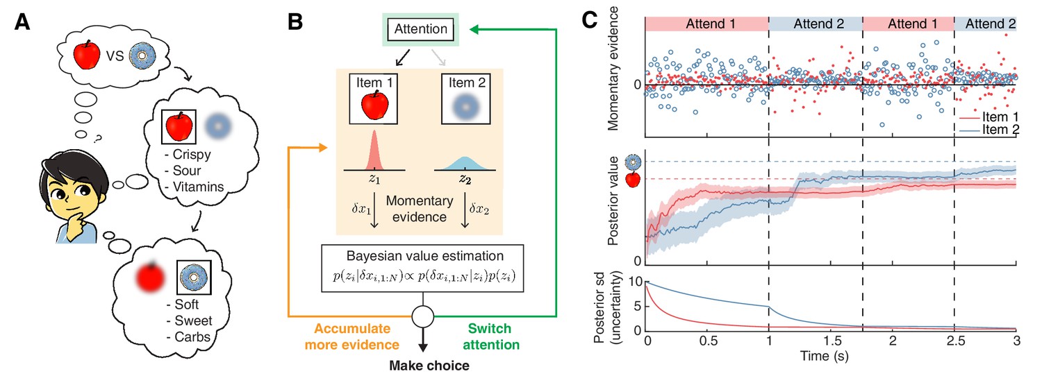
Attention-modulated evidence accumulation.

(A) Schematic depicting the value-based decision-making model. When choosing between two snack items (e.g. apple versus donut), people tend to evaluate each item in turn, rather than think about all items simultaneously. While evaluating one item, they will pay less attention to the unattended item (blurred item). (B) Schematic of the value-based decision process for a single decision trial. At trial onset, the model randomly attends to one item (green box). At every time step, it accumulates momentary evidence (orange box) that provides information about the true value of each item, which is combined with the prior belief of each item’s value to generate a posterior belief. Note that the momentary evidence of the attended item comes from a tighter distribution. Afterwards, the model assesses whether to accumulate more evidence (orange), make a choice (black), or switch attention to the other item (green). (C) Evolution of the evidence accumulation process. The top panel shows momentary evidence at every time point for the two items. Note that evidence for the unattended item has a wider variance. The middle panel shows how the posterior estimate of each item may evolve over time (mean ± 1SD). The horizontal dotted lines indicate the unobserved, true values of the two items. The bottom panel shows how uncertainty decreases regarding the true value of each item. As expected, uncertainty decreases faster for the currently attended item compared to the unattended one. For this descriptive figure, we used the following parameters: $z = [13, 10]$ , $σ_{x}^{2} = 5$ , $σ_{z}^{2} = 10$ , $γ = 0.1$ , $δ t = 0.01$ .

Figure 2 with 1 supplement

Download asset Open asset

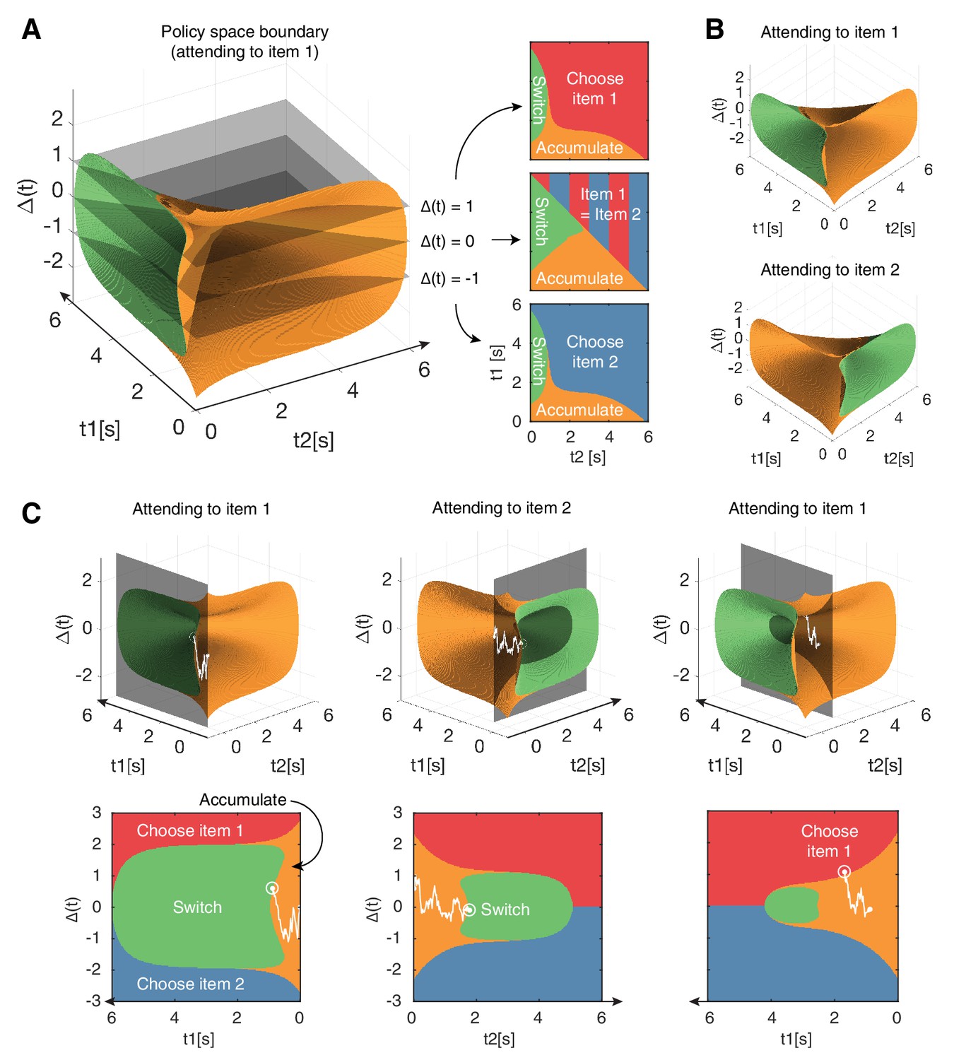
Navigating the optimal policy space.

(A) The optimal policy space. The policy space can be divided into regions associated with different optimal actions (choose item 1 or 2, accumulate more evidence, switch attention). The boundaries between these regions can be visualized as contours in this space. The three panels on the right show cross-sections after slicing the space at different $Δ$ values, indicated by the gray slices in the left panel. Note that when $Δ = 0$ (middle panel), the two items have equal value and therefore there is no preference for one item over the other. (B) Optimal policy spaces for different values of $y$ (currently attended item). The two policy spaces are mirror-images of each other. (C) Example deliberation process of a single trial demonstrated by a particle that diffuses across the optimal policy space. In this example, the model starts by attending to item 1, then makes two switches in attention before eventually choosing item 1. The bottom row shows the plane in which the particle diffuses. Note that the particle diffuses on the (gray, shaded) plane perpendicular to the time axis of the unattended item, such that it only increases in t_j when attending to item j. Also note that the policy space changes according to the item being attended to, as seen in (B). See results text for more detailed description. See Figure 2—figure supplement 1 to view changes in the optimal policy space depending on changes to model parameters.

Figure 2—figure supplement 1

Download asset Open asset

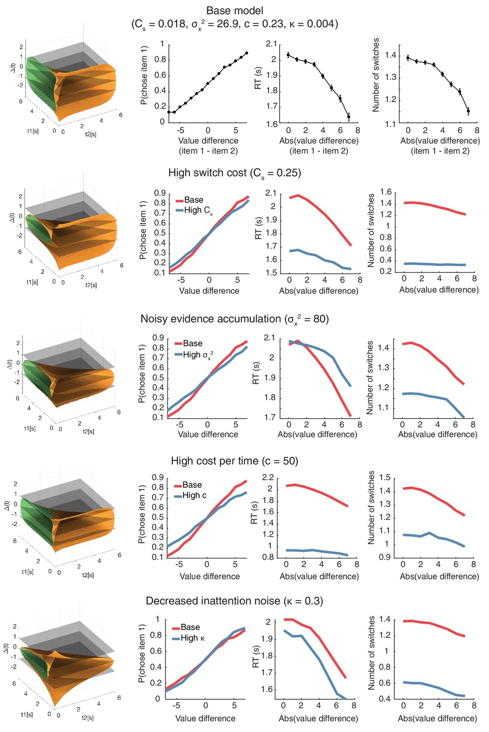
Changes in the optimal policy space and model behavior with adjustments in free model parameters.

Changes in the optimal policy space and model behavior with adjustments in free model parameters. The optimal policy space and its associated psychometric curves from the base model are shown in the top row. The policy space and psychometric curves corresponding to changes in single free parameters are shown in subsequent rows. In rows 2–4, psychometric curves from the base model on row 1 is shown in red for comparison.

Figure 3 with 2 supplements

Download asset Open asset

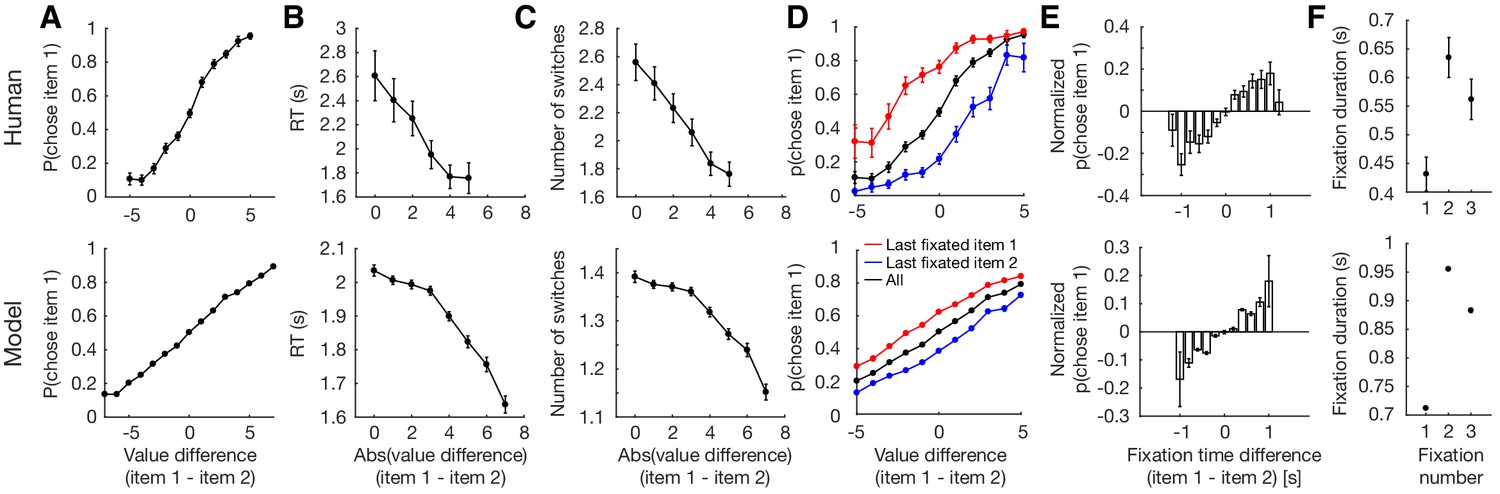
Replication of human behavior by simulated optimal model behavior (Krajbich et al., 2010).

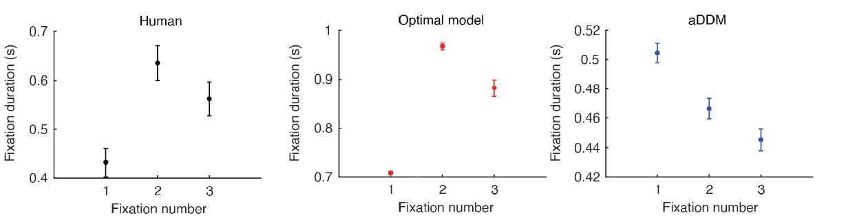
(A) Monotonic increase in probability of choosing item 1 as a function of the difference in value between item 1 and 2 ( $t (38) = 105.7, p < 0.001$ ). (B) Monotonic decrease in response time (RT) as a function of trial difficulty ( $t (38) = - 11.1, p < 0.001$ ). RT increases with increasing difficulty. (C) Decrease in the number of attention switches as a function of trial difficulty. More switches are made for harder trials ( $t (38) = - 8.10, p < 0.001$ ). (D) Effect of last fixation location on item preference. The item that was fixated on immediately prior to the decision was more likely to be chosen. (E) Attention’s biasing effect on item preference. The item was more likely to be chosen if it was attended for a longer period of time ( $t (38) = 5.32, p < 0.001$ ). Since the probability of choosing item 1 depends on the degree of value difference between the two items, we normalized the p(choose item 1) by subtracting the average probability of choosing item 1 for each difference in item value. (F) Replication of fixation pattern during decision making. Both model and human data showed a fixation pattern where a short initial fixation was followed by a longer, then medium-length fixation. Error bars indicate standard error of the mean (SEM) across both human and simulated participants ( $N = 39$ for both). See Figure 3—figure supplement 2 for an analogous figure for the perceptual decision task.

Figure 3—figure supplement 1

Download asset Open asset

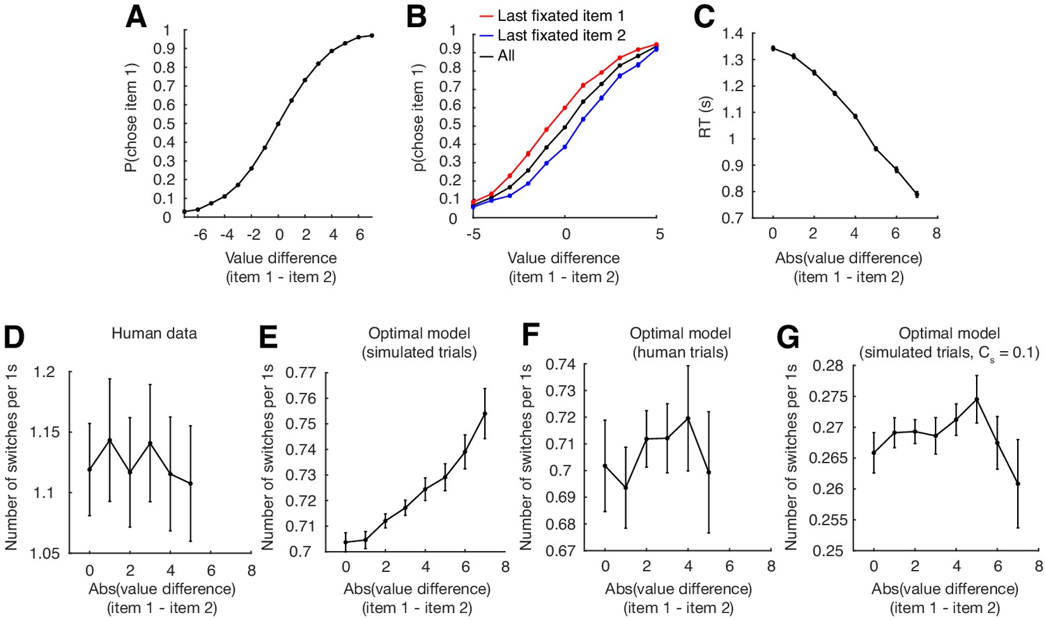
Parameter-dependence of psychometric/chronometric curves, and exploration of switch rate rather than switch number for the optimal model.

Parameter-dependence of psychometric/chronometric curves, and exploration of switch rate rather than switch number for the optimal model. (A–C) Psychometric (A,B) and chronometric (C) curves after decreasing the evidence noise term ( $σ^{2}$ ) from 27 to 5. Figure 3 suggests a qualitative difference in psychometric/chronometric curves between human and model behavior. For Figure 3A,D, the model’s psychometric curve appeared linear rather than sigmoidal. To show that this is a result of the difficulty of the task, as determined by the evidence noise term ( $σ^{2}$ ), and not a generalizable property of the model, we set ( $σ^{2}$ ) in (A) and (B) to a lower value, in which case the model exhibits sigmoidal psychometric curves. This sigmoidal shape arises because the decision becomes easier at extreme value differences and approaches perfect performance. In Figure 3B, the model’s chronometric curve had a concave shape, whereas that of the humans appeared linear. As (C) shows, decreasing the noise term diminished, but did not eliminate this concave shape. (D) Human switch rate (number of switches divided by time) did not change significantly with trial difficulty ( $t (38) = - 0.32, p = 0.75$ ). (E) In the optimal model, it significantly increased with a decrease in task difficulty ( $t (38) = 2.96, p = 0.0052$ ). (F) This relationship ceases to be apparent once we reduce the number of simulated trials to that of the human data ( $t (38) = 1.02, p = 0.31$ ), suggesting the human data may be underpowered to show such a relationship. (G) The relationship between switch rate and trial difficulty is not a general property of the optimal model, as a significant increase in the switch cost (adjusting $C_{s}$ from 0.018 to 0.1) removes the effect seen in (E) ( $t (38) = - 0.50, p = 0.62$ ), even with a large number of simulated trials. Error bars indicate SEM across participants.

Figure 3—figure supplement 2

Download asset Open asset

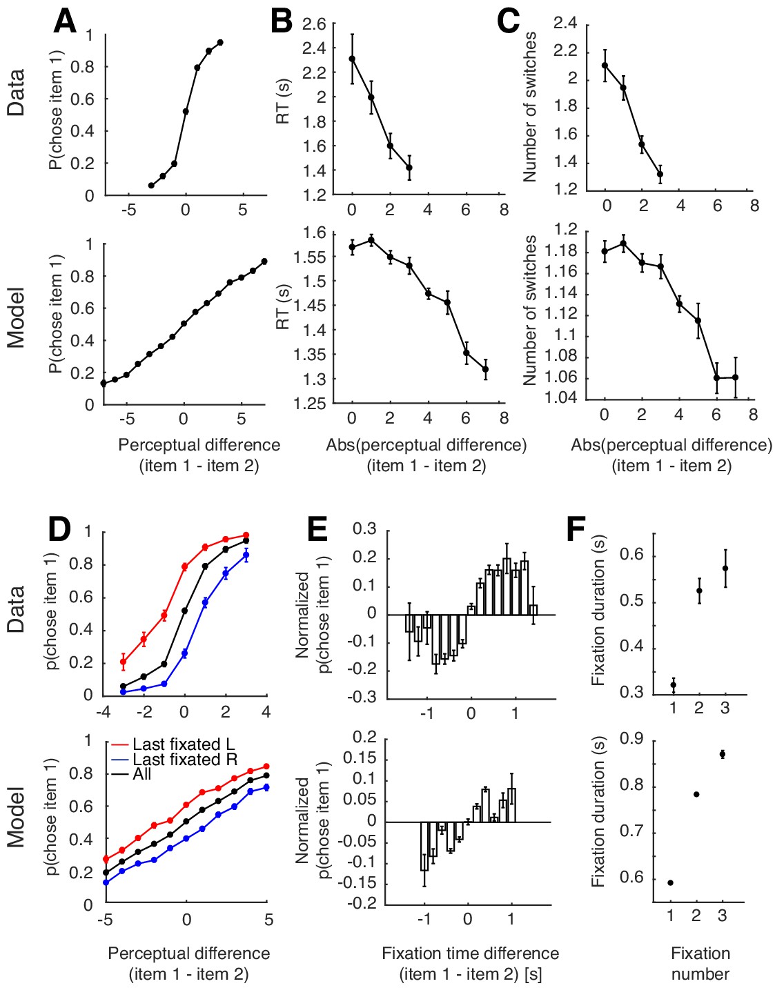
Replicating human perceptual decision-making behavior with the optimal model.

Replicating human perceptual decision-making behavior with the optimal model. In each trial of the perceptual decision task used in Tavares et al., 2017, human decision makers had to identify which of two presented lines were closer in orientation to a preceding target orientation. To model this decision, the authors assumed that the decision maker compares the difference in perceptual quality (i.e. angle of a line; 0°, 5°, 10°, 15°) between the target and the two lines, then converted this difference to a scale ranging from 0 to 3 with three denoting the best possible proximity (i.e. 0°). Following this, we simulated the task such that our model accumulates noisy evidence centered around the perceptual difference scale (0–3) between the target and the two lines, and chose the item with a larger value using this scale (see Appendix 1). (A) Monotonic increase in probability of choosing item 1 as a function of the perceptual difference between item 1 and 2. (B) Decrease in response time (RT) as a function of trial difficulty. (C) Decrease in the number of switches as a function of trial difficulty. (D) Effect of last fixation location on item preference. The item that was fixated on immediately prior to the decision was more likely to be chosen. (E) Attention’s biasing effect on item choice. The item was more likely to be chosen if it was attended to for a longer period of time. (F) Replication of fixation pattern during decision making. In the perceptual decision-making task, both model and human data showed increased duration for every subsequent fixation, a notable difference compared to fixation behavior in the value-based task. For (A–D), the behavioral data has a smaller range of perceptual differences due to insufficient trials with such large perceptual difference. Error bars indicate SEM across participants.

Figure 4 with 3 supplements

Download asset Open asset

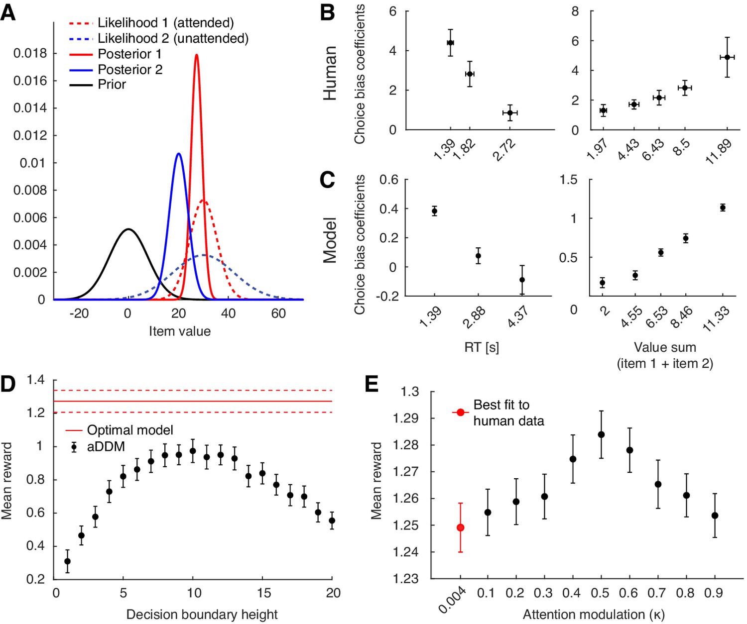
Behavioral predictions from Bayesian value estimation, and further properties of the optimal policy.

(A) Bayesian explanation of attention-driven value preference. Attending to one of two equally-valued items for a longer time (red vs. blue) leads to a more certain (i.e. narrower) likelihood and weaker bias of its posterior towards the prior. This leads to a subjectively higher value for the longer attended item. (B) Effect of response time (RT; left panel; $t (38) = - 3.25, p = 0.0024$ ) and sum of the two item values (value sum; right panel; $t (38) = 2.95, p = 0.0054$ ) on attention-driven choice bias in humans. This choice bias quantifies the extent to which fixations affect choices for the chosen subset of trials (see Materials and methods). (C) Effect of response time (left panel; $t (38) = - 32.0, p < 0.001$ ) and sum of the two item values (right panel; $t (38) = 11.4, p < 0.001$ ) on attention-driven choice bias in the optimal model. See Materials and methods for details on how the choice bias coefficients were computed. For (B) and (C), for the left panels, the horizontal axis is binned according to the number of total fixations in a given trial. For the right panels, the horizontal axis is binned to contain the same number of trials per bin. Horizontal error bars indicate SEM across participants of the mean x-values within each bin. Vertical error bars indicate SEM across participants. (D) Comparing decision performance between the optimal policy and the original aDDM model. Performance of the aDDM was evaluated for different boundary heights (error bars = SEM across simulated participants). Even for the reward-maximizing aDDM boundary height, the optimal model significantly outperformed the aDDM ( $t (38) = 3.01, p = 0.0027$ ). (E) Decision performance for different degrees of the attention bottleneck ( $κ$ ) while leaving the overall input information unchanged (error bars = SEM across simulated participants). The performance peak at $κ = 0.5$ indicates that allocating similar amounts of attentional resource to both items is beneficial ( $t (38) = - 8.51, p < 0.001$ ).

Figure 4—figure supplement 1

Download asset Open asset

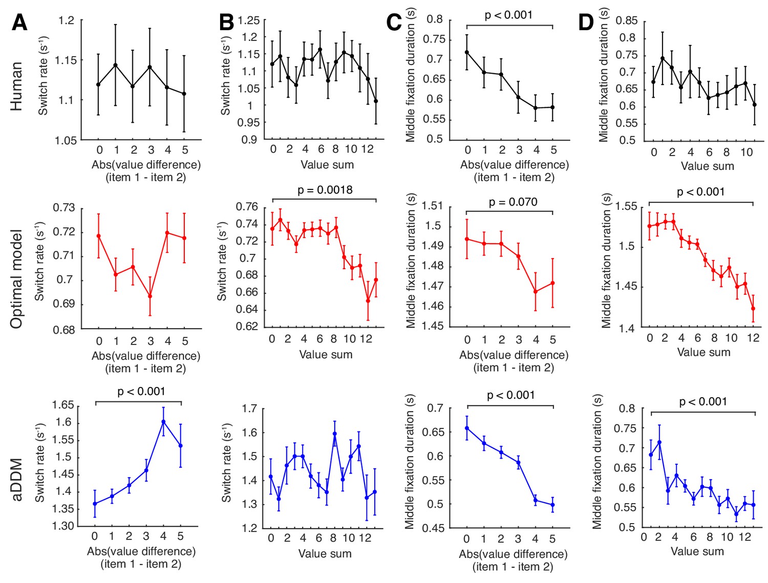
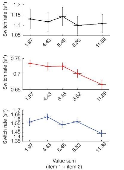
Effect of item values on attention switch rate and fixation duration across trials for the human data, optimal model, and aDDM.

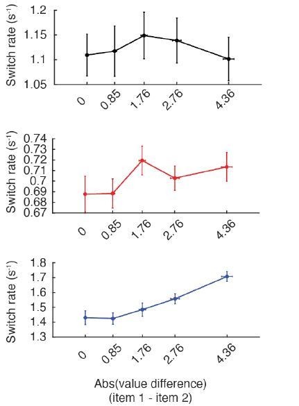
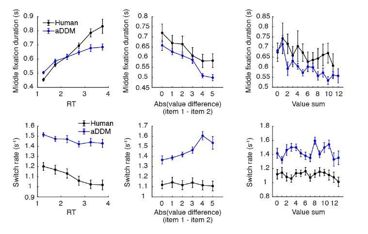
Effect of item values on attention switch rate and fixation duration across trials for human data, optimal model, and aDDM. (A) Effect of absolute value difference (i.e. trial difficulty) on switch rate. Only the aDDM showed a significant dependence of switch rate on difficulty, featuring a higher switch rate for less difficult trials ( $t (38) = 4.97, p < 0.001$ ). (B) Relationship between value sum and switch rate. A larger value sum led to a smaller switch rate for the optimal model ( $t (38) = - 3.36, p = 0.0018$ ). Human data showed a non-significant trend in the same direction ( $t (38) = - 1.31, p = 0.20$ ). (C) Dependence of middle fixation duration on absolute value difference. Humans and both models featured shorter fixation duration in easier trials (human: $t (38) = - 4.15, p < 0.001$ ; optimal model: $t (38) = - 2.85, p = 0.0070$ ; aDDM: $t (38) = - 6.52, p < 0.001$ ). (D) Dependence of middle fixation duration on value sum. Both the optimal model and the aDDM featured shorter fixation durations for larger value sums (optimal model: $t (38) = - 4.06, p < 0.001$ ; aDDM: $t (38) = - 4.34, p < 0.001$ ). Human data featured a non-significant trend in the same direction ( $t (38) = - 1.53, p = 0.13$ ). For all plots, we computed the mean switch rate (number of switches divided by RT) and middle fixation duration for every trial, then grouped the trials by absolute value difference (i.e. trial difficulty) or value sum. We then computed the mean switch rate and fixation duration across participants for each x-variable. Curves with a slope significantly different from zero are indicated by a bar above the curve with its associated p-value (see Materials and methods for statistics involving slopes). For both model’s simulations, we used the same item pairs and trial numbers as the human data. For the aDDM simulations, we used the same parameter setup used in the original paper by Krajbich et al., 2010 rather than the signal-to-noise-matched version we used to compare the mean reward between the optimal model and aDDM. Error bars indicate SEM across participants.

Figure 4—figure supplement 2

Download asset Open asset

Effect of passed time on switch probability and fixation duration within trials.

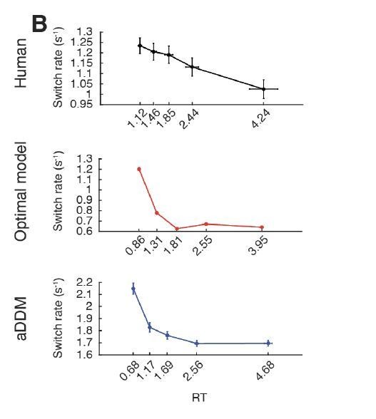
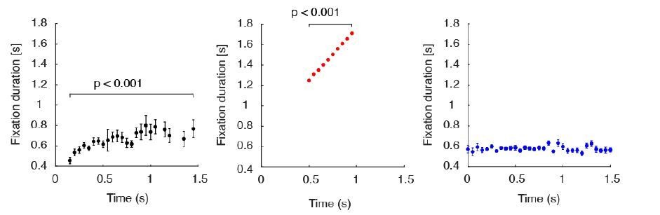
Effect of passed time on switch probability and fixation duration within trials. (A) Effect of passed time on switch probability, using all trials. Switch probability for humans and aDDM peaked within 1 s of stimulus onset and gradually decreased thereafter. For the optimal model, the majority of attention switches were clustered around discrete time points. Note that the optimal model assumes the decision maker to use precise time estimates to drive attention switches. If we were to take into account the noisiness of human choice estimates (Buhusi and Meck, 2005), we would expect the optimal model curves to smoothen out and approach those of human data and the aDDM. (B–D) Effect of passed time on switch probability after dividing trials into upper and lower one-third of certain variables (B: RT, C: value sum, D: absolute value difference). When trials are split by RT (B), humans and aDDM featured a higher switch probability for longer (i.e. higher RT) trials. The optimal model featured comparable patterns within the time periods in which switches occurred. The dashed line indicates the point in time in which all trials were completed for the lower RT group. (E) Effect of passed time on fixation duration. Fixation duration increased with passed time for humans and the optimal model, suggesting that more time is allotted to each fixation as the trial becomes more difficult (human: $t (38) = 4.50, p < 0.001$ ; optimal model: $t (38) = 46.4, p < 0.001$ ). This trend is not seen in the aDDM which draws all middle fixations randomly from the same empirical distribution, therefore eliminating any effect of time on fixation duration within a single trial ( $t (38) = - 0.57, p = 0.57$ ). To compute the switch probability (A–D), we aligned all trials within each participant by stimulus onset, then counted the number of switches within each 0.2 s time bin. We then averaged the switch count in each time bin across trials to compute the switch probability. We only included time points up to when at least 1/3 of the total trials are included, and removed the last fixations since they are prematurely terminated when a decision is made. To split trials based on different variables, all trials within a participant were split into three equally sized bins based on the variable of interest. We plot the mean switch probability across participants, only including the first (green) and last (magenta) bins. At each time point, we performed a t-test across participants between the two bins, and marked all time points with a significant difference across bins with an asterisk (Bonferroni corrected; Bonferroni, 1936). For (E), whenever a new fixation occurred, we recorded its duration until the next fixation, excluding the first and last fixations. We averaged the fixation durations at each 0.05 s time bin across trials, dropping any time bin that contain data from less than 1/3 of all trials. We then plotted the mean fixation duration at each time bin across participants. Error bars indicate SEM across participants.

Figure 4—figure supplement 3

Download asset Open asset

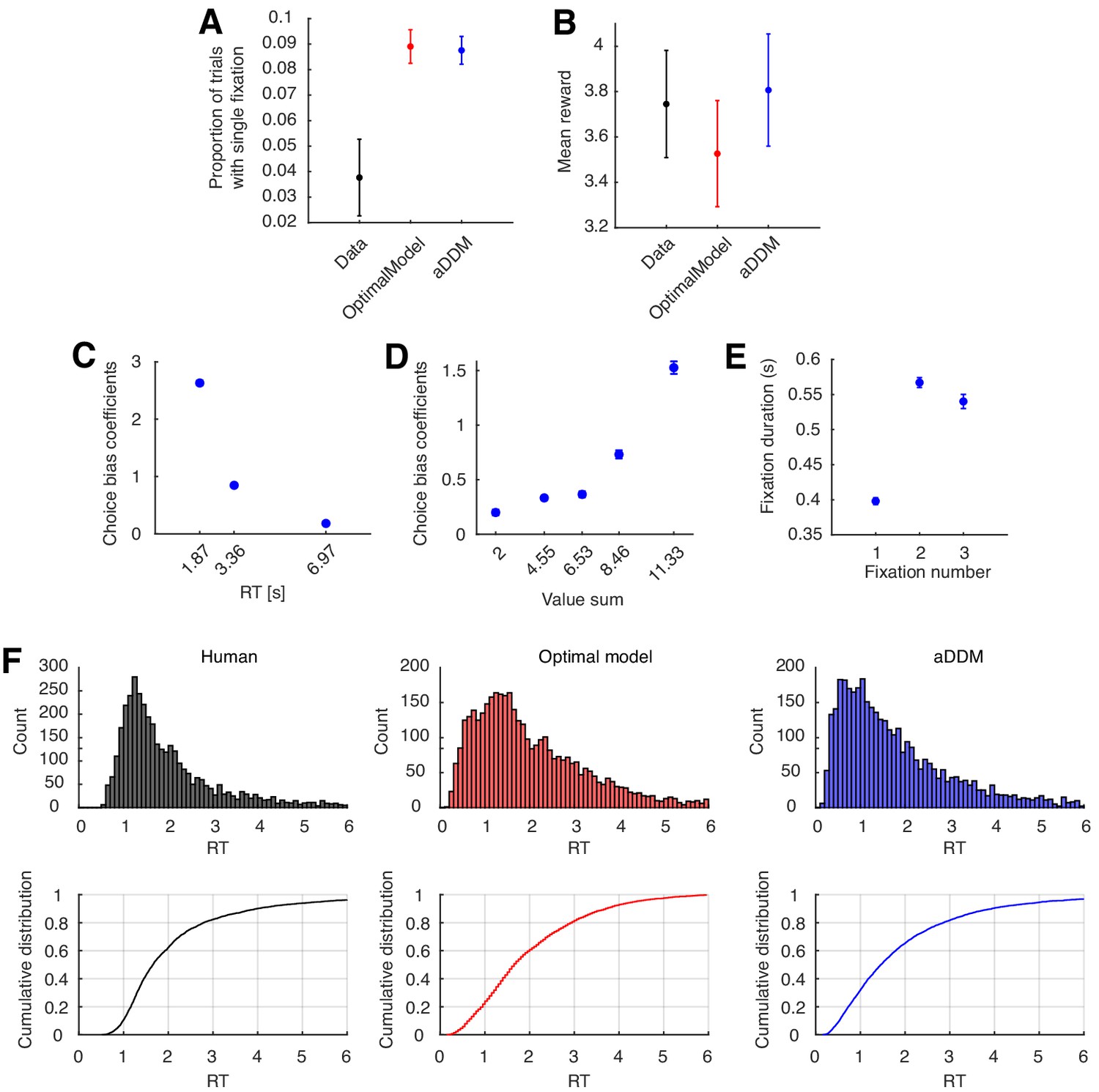
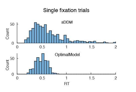
Additional analyses of fixation behavior and performance between human data, optimal model, and aDDM.

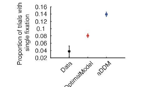
Additional analyses of fixation behavior, performance, and choice bias between human data, optimal model, and aDDM. (A) Proportion of all trials that ended after a single fixation. Both the optimal model and aDDM featured more single fixation trials when compared to human data (optimal model: $t (76) = 2.96, p = 0.0052$ ; aDDM: $t (76) = 3.35, p = 0.0019$ ). (B) Comparing the mean reward received by humans versus the two models using the best-fitting model parameters. There was no significant difference between the mean rewards of humans versus either model (optimal model: $t (76) = 0.69, p = 0.49$ ; aDDM: $t (76) = - 0.062, p = 0.95$ ). Unlike in Figure 4D, the mean reward of the optimal model was not larger than the aDDM in this scenario because we simulated the aDDM using the original parameters rather than those that match the optimal model’s signal-to-noise ratio of the momentary evidence. To calculate mean reward, we used the same cost per unit time used for the optimal model ( $c = 0.23$ ). For model simulations in (A) and (B), we used three times as many trials as performed by humans. (C,D) Effect of RT (C) and value sum (D) on choice bias in the aDDM. The aDDM also replicated the same effects as predicted by the optimal model (RT: $t (38) = - 48.6, p < 0.001$ ; value sum: $t (38) = 14.7, p < 0.001$ ). For both plots, trial data were binned into equally sized bins based on the variable on the x-axis. See Materials and methods for how to compute the choice bias coefficient. (E) Mean fixation duration of the first three fixations across simulated aDDM participants. Since the fixation durations in the aDDM are sampled from the empirical distribution, it closely mimics those from human data. (F) Distribution of response times. Both models predict an RT distribution that seem to include more trials with RT <1 s. For the aDDM simulations, we used the same parameter setup used in the original paper by Krajbich et al., 2010. For (A–E), vertical error bars indicate SEM across participants. For (C) and (D), horizontal error bars indicate the SEM of the bin means.

Author response image 1

Download asset Open asset

Author response image 2

Download asset Open asset

Author response image 3

Download asset Open asset

Author response image 4

Download asset Open asset

Author response image 5

Download asset Open asset

Author response image 6

Download asset Open asset

Author response image 7

Download asset Open asset

Author response image 8

Download asset Open asset

Author response image 9

Download asset Open asset

Author response image 10

Download asset Open asset

Additional files

Source data 1 Human behavioral data readme.: https://cdn.elifesciences.org/articles/63436/elife-63436-data1-v2.zip
Download elife-63436-data1-v2.zip
Source data 2 Human behavioral data.: https://cdn.elifesciences.org/articles/63436/elife-63436-data2-v2.zip
Download elife-63436-data2-v2.zip
Transparent reporting form: https://cdn.elifesciences.org/articles/63436/elife-63436-transrepform-v2.docx
Download elife-63436-transrepform-v2.docx

Download links

A two-part list of links to download the article, or parts of the article, in various formats.

Downloads (link to download the article as PDF)

Open citations (links to open the citations from this article in various online reference manager services)

Mendeley

Cite this article (links to download the citations from this article in formats compatible with various reference manager tools)

Anthony I Jang
Ravi Sharma
Jan Drugowitsch

(2021)

Optimal policy for attention-modulated decisions explains human fixation behavior

eLife 10:e63436.

https://doi.org/10.7554/eLife.63436

Sign up for email alerts

Privacy notice