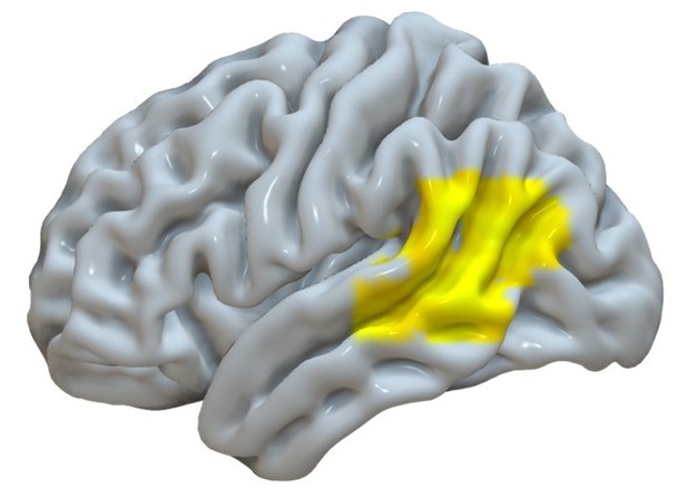
Temporo-parietal cortex involved in modeling one’s own and others’ attention
Figures
Methods.
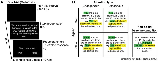
(A) Schematic timeline of the fMRI design. In each trial, subjects were presented with a short story for 10 s, describing a scene in which an agent attended to an object in the environment. A probe statement was then shown for 4 s, relating to either the story’s spatial context or object property, to which the subjects responded either true or false by button press. (B) The agent in the story was either the subject him-/herself (self) or another person (other), and directed attention to the object endogenously (internally driven attention) or exogenously (stimulus-driven attention), yielding a 2 × 2 factorial design of attention type × agent. We created 80 unique stories in four different versions, one for each condition. We made minimal changes to the wordings to keep the story versions as semantically similar as possible. Green highlighting indicates wording specifying agent, yellow highlighting indicates wording specifying attention type (colors not part of actual visual stimuli). For each story, each subject saw only one of the four versions (balanced across subjects). We also included a nonsocial control condition (20 unique stories based on a subset of the 80 social stories) in which the agent was replaced by a non-human object.
Regions of interest (ROIs).
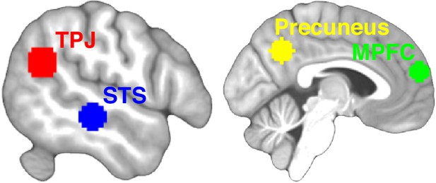
Six ROIs were defined based on peaks reported in an activation likelihood estimation meta-analysis of 16 fMRI studies involving theory-of-mind reasoning (van Veluw and Chance, 2014). The ROIs consisted of 10-mm-radius spheres centered on peaks in the bilateral temporoparietal junction (TPJ) and superior temporal sulcus (STS), and two midline structures: the precuneus and medial prefrontal cortex (MPFC). Here, the TPJ and STS ROIs on the left side are shown.
Decoding attention type, agent, and the interaction between them, in six brain areas.
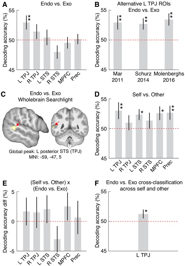
For definition of ROIs, see Figure 2. Each point shows mean decoding accuracy. Error bars show SEM. Red horizontal line indicates chance level decoding. Significance indicated by * (p<0.05) and ** (p<0.01), based on permutation testing (all significant p values also survived FDR correction for multiple comparisons across all six ROIs [all significant corrected ps <0.05]). (A) The ability of a classifier, trained on BOLD activity patterns within each ROI, to decode endogenous (endo) versus exogenous (exo) attention. (B) To test the robustness of the endo-versus-exo decoding in the left TPJ, we replicated the results in three ROIs derived from theory-of-mind neuroimaging meta-analyses (Mar, 2011; Molenberghs et al., 2016; Schurz et al., 2014) other than the one used for the main analysis (van Veluw and Chance, 2014) (see Figure 3—figure supplement 2 for details). (C) The cluster shown had the highest decoding accuracy in the whole-brain, searchlight analysis, for the endo-versus-exo comparison. No clusters in this analysis survived brain-wide correction for multiple comparisons. We here report clusters surviving the conventional uncorrected voxelwise threshold p<0.001, for purely descriptive purposes. See Figure 3—figure supplement 3 and Supplementary file 1 for details. (D) Decoding accuracy for agent (self versus other). (E) Decoding accuracy for the interaction between type of attention and agent. (F) The ability of a classifier, trained to discriminate attention type in self stories, to decode attention type in other stories, and vice versa (i.e. two-way cross-classification), based on activity patterns in the left TPJ ROI.
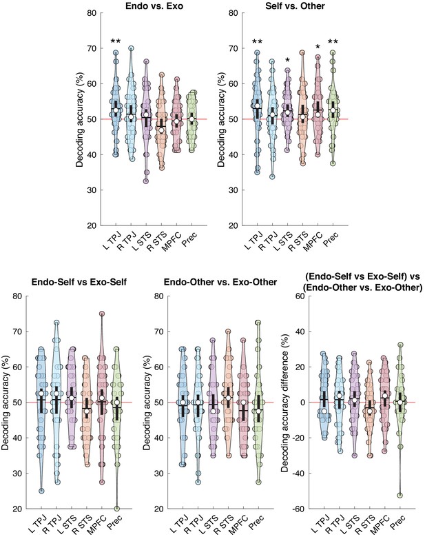
Decoding attention type, agent, and the interaction between the two, within the six ROIs.
Violin plots showing mean (black horizontal line) and median (white circle) decoding accuracy (%), 95% confidence interval around the mean based on bootstrap distribution (black vertical line), a kernel density estimation (shaded area), and individual data points for each of the six ROIs. The horizontal red line indicates chance decoding. *p<0.05, **p<0.01.
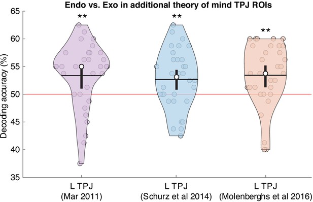
Replicating attention type decoding results in additional TPJ ROIs.
To test the robustness of the endogenous-versus-exogenous decoding in the left TPJ, we replicated the results in three ROIs derived from theory-of-mind neuroimaging meta-analyses (Mar, 2011; Molenberghs et al., 2016; Schurz et al., 2014) other than the one used for the main analysis (van Veluw and Chance, 2014). The ROIs were defined as 10-mm-radius spheres around the peak left TPJ coordinates reported in Mar, 2011 (MNI: −53,–56, 22), Schurz et al., 2014 (MNI: −55,–59, 20), and Molenberghs et al., 2016 (MNI: −52,–58, 22). The results showed significant decoding in the Mar ROI (mean decoding accuracy 53.4%, 95% CI 51.0–55.1, p=0.0023), the Schurz ROI (mean decoding accuracy 52.7%, 95% CI 50.8–54.4, p=0.0092), and in the Molenberghs ROI (mean decoding accuracy 53.4%, 95% CI 51.3–55.2, p=0.0020). Violin plots show mean (black horizontal line) and median (white circle) decoding accuracy (%), 95% confidence interval around the mean based on bootstrap distribution (black vertical line), a kernel density estimation (shaded area), and individual data points for the two ROIs. The red horizontal line indicates chance decoding. **p<0.01.
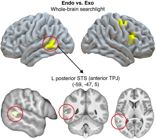
Decoding attention type at the whole-brain level.
The cluster shown had the highest decoding accuracy in the whole-brain, searchlight analysis, for the endogenous-versus-exogenous comparison. See Supplementary file 1 for numerical details. Top: projected onto a 3D canonical brain surface. Bottom: projected onto sections of the average structural scan generated from the 32 subjects for anatomical localization. For display purposes, the statistical threshold for the activation maps was set to p<0.001, uncorrected.
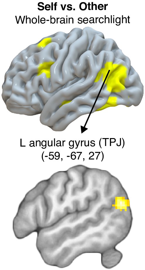
Decoding agent type at the whole-brain level.
The cluster shown had the highest decoding accuracy in the whole-brain, searchlight analysis, for the self-versus-other comparison. See Supplementary file 2 for numerical details. Top: projected onto a 3D canonical brain surface. Bottom: projected onto a parasagittal section of the average structural scan generated from the 32 subjects for anatomical localization. For display purposes, the statistical threshold for the activation maps was set to p<0.001, uncorrected.
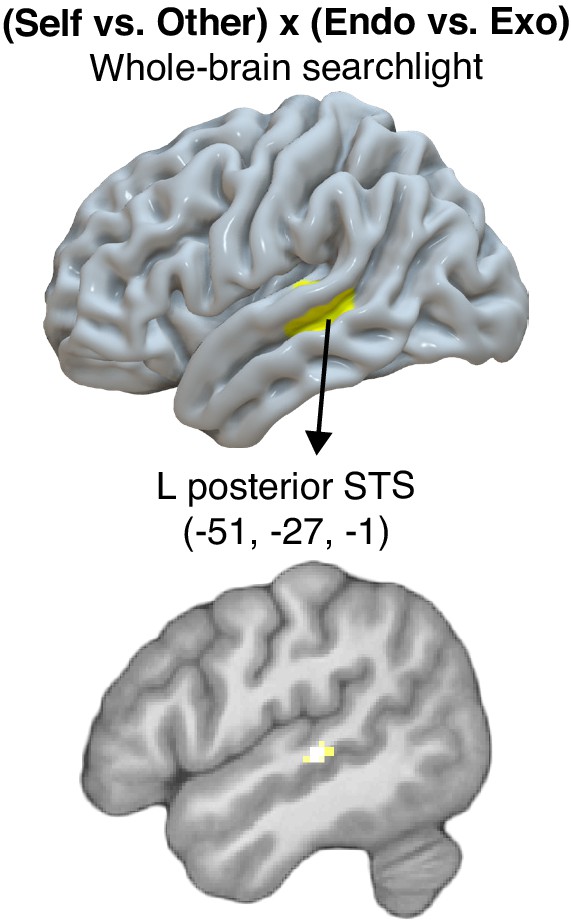
Decoding attention-by-agent interaction at the whole-brain level.
The cluster shown had the highest decoding accuracy difference in the whole-brain, searchlight analysis, for the (endogenous-versus-exogenous)SELF versus (endogenous-versus-exogenous)OTHER comparison. See Supplementary file 3 for numerical details. Top: projected onto a 3D canonical brain surface. Bottom: projected onto a parasagittal section of the average structural scan generated from the 32 subjects for anatomical localization. For display purposes, the statistical threshold for the activation maps was set to p<0.001, uncorrected.
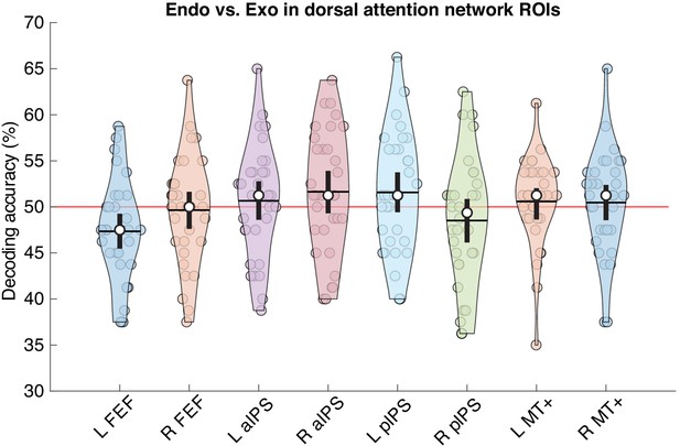
Decoding attention type in the dorsal attention network.
The TPJ is part of the ventral attention network, which has been implicated in exogenous attention. Could it be the case that participants simulate attention orienting when reading the stories, leading to the above-chance endogenous-versus-exogenous decoding in the TPJ? If this is the case, one should expect above-chance decoding also in areas of the dorsal attention network, which has been implicated in endogenous attention. To test this hypothesis, we replicated the endogenous-versus-exogenous analysis in four areas (bilaterally) typically considered to constitute the dorsal attention network: the frontal eye fields (FEF), the anterior and posterior intraparietal sulcus (aIPS and pIPS), and the middle temporal complex (MT+). The ROIs were defined as 10-mm-radius spheres around the peak coordinates (reported in Fox et al., 2006): left FEF (MNI: −25,–16, 61), right FEF (MNI: 27,–14, 58), left aIPS (MNI: −42,–44, 46), right aIPS (MNI: 34,–51, 49), left pIPS (MNI: −22,–72, 51), right pIPS (MNI: 19,–72, 57), left MT+ (MNI: −47,–68, −14), and right MT+ (MNI: 51,–63, −14). The results showed that none of the dorsal attention network ROIs decoded the attention type in the stories better than chance (all ps > 0.05, based on permutation testing with 10,000 iterations, uncorrected for multiple comparisons). Violin plots show mean (black horizontal line) and median (white circle) decoding accuracy (%), 95% confidence interval around the mean based on bootstrap distribution (black vertical line), a kernel density estimation (shaded area), and individual data points. The red horizontal line indicates chance decoding.
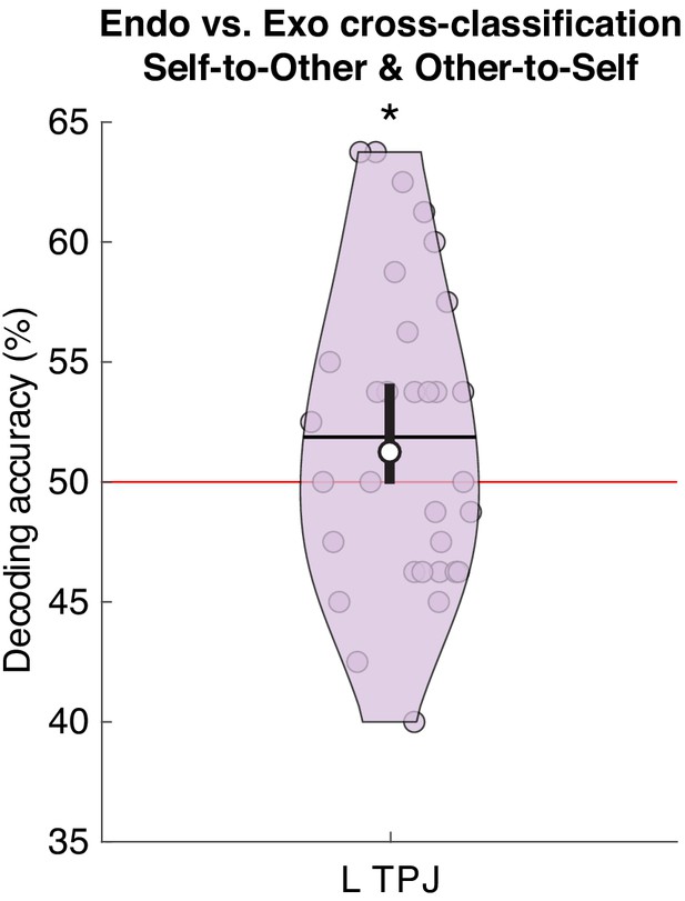
Decoding of attention type generalizes across self-stories and other-stories.
Violin plot showing the mean (black horizontal line) and median (white circle) decoding accuracy (%), 95% confidence interval around the mean based on bootstrap distribution (black vertical line), a kernel density estimation (shaded area), and individual data points for a two-way cross-classification analysis based on activity patterns in the left TPJ ROI. The red horizontal line indicates chance decoding. *p<0.05.
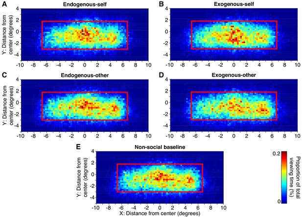
Eye tracking results.
Subjects tended to fixate in a similar spatial pattern across the screen, and engage in similar saccade dynamics, regardless of the type of story presented. No significant ability to decode the story type based on the pattern of eye movement was obtained. The red rectangle in the heat maps in panels A-E indicates the area of the screen within which the story text appeared.
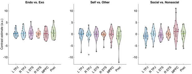
Univariate fMRI results within ROIs.
The difference in average activity across all voxels within each ROI, for the endogenous-versus-exogenous, self-versus-other, and social-versus-nonsocial contrasts, are shown. Violin plot showing the mean (colored horizontal line) and median (white circle) contrast estimate, interquartile range (black vertical line), a kernel density estimation (shaded area), and individual data points. None of the contrasts were statistically significant after controlling for multiple comparisons across all six ROIs (all FDR-corrected ps >0.21).
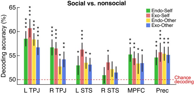
Decoding social versus nonsocial stories.
The ability of a classifier, trained on BOLD activity patterns within each of the six ROIs, to decode each of the four social story conditions (endogenous-self, exogenous-self, endogenous-other, and exogenous-other) versus the nonsocial control. Each bar shows mean decoding accuracy, error bars show SEM, red horizontal line shows chance level decoding. Significance indicated by * (p<0.05), ** (p<0.01), and *** (p<0.001) based on permutation testing (all but one of the significant p values also survived FDR correction for multiple comparisons across all six ROIs; see Table 3 for numerical details).
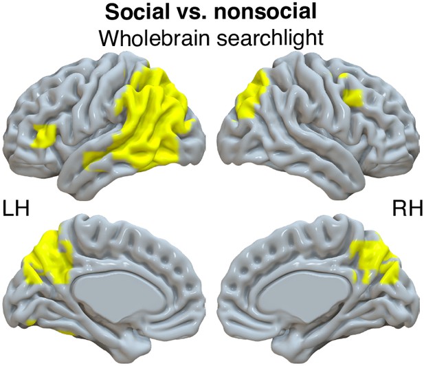
Decoding social versus nonsocial stories at the whole-brain level.
The clusters shown are areas of overlap between four whole-brain, searchlight analyses, for the social-versus-nonsocial comparison (endogenous-self versus nonsocial, exogenous-self versus nonsocial, endogenous-other versus nonsocial, exogenous-other versus nonsocial). See Supplementary file 4 for numerical details. Projected onto a 3D canonical brain surface.
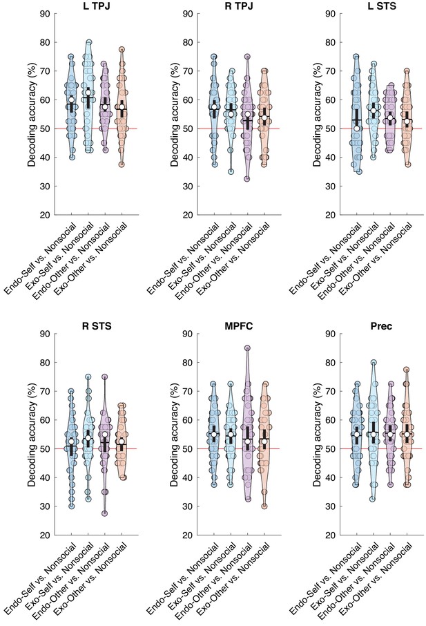
Decoding social versus nonsocial stories within the six ROIs.
Violin plots showing mean (black horizontal line) and median (white circle) decoding accuracy (%), 95% confidence interval around the mean based on bootstrap distribution (black vertical line), a kernel density estimation (shaded area), and individual data points for each of the six ROIs. The horizontal red line indicates chance decoding.
Tables
Behavioral results.
Mean accuracy and latency for the probe question that was presented after each story, for each of the five experimental conditions. The mean accuracy and latency across all social story conditions are also reported.
| Story type | Self-endo | Self-exo | Other-endo | Other-exo | Non-social | Social (all) | |
|---|---|---|---|---|---|---|---|
| Accuracy (%) | Mean | 94.2 | 93.4 | 93.1 | 93.4 | 90.0 | 93.6 |
| SEM | 1.9 | 1.8 | 1.6 | 1.9 | 2.2 | 1.4 | |
| Latency (ms) | Mean | 1613 | 1601 | 1667 | 1653 | 1957 | 1634 |
| SEM | 54 | 56 | 46 | 56 | 63 | 49 |
Decoding attention type, agent, and the interaction between the two, within the six ROIs.
For definition of ROIs, see Figure 2. Mean decoding accuracy (%), 95% confidence interval (based on bootstrap distribution), and p value (based on permutation testing) are shown for each of the six ROIs. Results shown for decoding endogenous (endo) versus exogenous (exo) attention type, self versus other agent type, and the interaction between the two variables. * indicates significant p values that survived correction for multiple comparisons across all six ROIs (FDR-corrected p<0.05).
| L TPJ | R TPJ | L STS | R STS | MPFC | Precuneus | ||
|---|---|---|---|---|---|---|---|
| Endo vs. Exo | Mean accuracy | 52.9% | 51.4% | 50.4% | 48.0% | 49.5% | 50.2% |
| 95% CI | 50.7–55.2 | 49.1–53.9 | 47.8–52.8 | 45.9–50.1 | 47.6–51.4 | 48.5–51.8 | |
| P value | 0.0046* | 0.1148 | 0.3518 | 0.9547 | 0.6439 | 0.4428 | |
| Self vs. Other | Mean accuracy | 53.0% | 51.0% | 52.3% | 51.3% | 52.6% | 52.7% |
| 95% CI | 50.1–55.6 | 48.5–53.4 | 50.6–54.1 | 48.9–54.1 | 50.5–55.0 | 50.4–55.0 | |
| P value | 0.0053* | 0.1974 | 0.0204* | 0.1241 | 0.0105* | 0.0099* | |
| (Self vs. Other) × (Endo vs. Exo) | Mean accuracy diff | 1.6% | 1.5% | 2.0% | −3.0% | 2.5% | 0.6% |
| 95% CI | −2.7–6.3 | −3.6–6.5 | −2.7–6.3 | −7.4–1.1 | −2.3–6.7 | −5.5–5.5 | |
| P value | 0.2430 | 0.2639 | 0.1967 | 0.8944 | 0.1414 | 0.3900 |
Decoding social versus nonsocial stories within the six ROIs.
For definition of ROIs, see Figure 2. Mean decoding accuracy (%), 95% confidence interval (based on bootstrap distribution), and p value (based on permutation testing) are shown for each of the six ROIs. Results shown for each of four social story conditions (endogenous-self, exogenous-self, endogenous-other, and exogenous-other) versus the nonsocial control. * indicates significant p values that survived correction for multiple comparisons across all six ROIs (FDR-corrected p<0.05).
| L TPJ | R TPJ | L STS | R STS | MPFC | Precuneus | ||
|---|---|---|---|---|---|---|---|
| Endo-Self vs. nonsocial | Mean accuracy | 58.5% | 56.7% | 53.0% | 50.9% | 55.2% | 54.6% |
| 95% CI | 55.5–61.6 | 53.5–59.8 | 49.3–56.8 | 47.5–54.0 | 52.3–58.0 | 51.5–57.7 | |
| p value | 0.0001* | 0.0001* | 0.0338* | 0.2703 | 0.0026* | 0.0027* | |
| Exo-Self vs. nonsocial | Mean accuracy | 60.7% | 56.5% | 56.3% | 53.6% | 54.5% | 55.7% |
| 95% CI | 57.0–64.4 | 53.7–58.8 | 53.5–59.0 | 50.5–56.6 | 51.7–57.1 | 51.9–59.4 | |
| p value | 0.0001* | 0.0002* | 0.0001* | 0.0179* | 0.0044* | 0.0001* | |
| Endo-Other vs. nonsocial | Mean accuracy | 58.4% | 52.7% | 53.5% | 52.2% | 53.4% | 55.4% |
| 95% CI | 55.9–60.9 | 49.6–55.9 | 51.1–55.9 | 48.8–55.0 | 49.5–57.7 | 52.6–58.2 | |
| p value | 0.0001* | 0.0497 | 0.0147* | 0.0969 | 0.0219* | 0.0014* | |
| Exo-Other vs. nonsocial | Mean accuracy | 56.7% | 54.2% | 53.1% | 51.5% | 53.4% | 55.2% |
| 95% CI | 53.8–59.8 | 51.1–57.3 | 50.4–55.9 | 49.1–54.0 | 49.8–56.7 | 52.0–58.5 | |
| p value | 0.0002* | 0.0065* | 0.0319* | 0.1901 | 0.0197* | 0.0012* |
Additional files
-
Supplementary file 1
Decoding endogenous versus exogenous at the whole-brain level.
All clusters (≥10 voxels) of decoding activity passing the voxelwise threshold of p<0.001 (none of the clusters survived p<0.05 correction for multiple comparisons using the whole brain as search space). *The left posterior STS cluster also coincided with the posterior TPJ (TPJp) subregion as defined by Bzdok et al., 2013; Mars et al., 2012.
- https://cdn.elifesciences.org/articles/63551/elife-63551-supp1-v1.docx
-
Supplementary file 2
Decoding agent type at the whole-brain level.
All clusters (≥10 voxels) decoding agent type (self versus other) activity at the threshold of p<0.001 (uncorrected). Corrected p values represent cluster-level correction using the whole brain as search space.
- https://cdn.elifesciences.org/articles/63551/elife-63551-supp2-v1.docx
-
Supplementary file 3
Decoding attention-by-agent interaction at the whole-brain level.
All clusters (≥10 voxels) in which endogenous-versus-exogenous decoding was better in self-related compared to other-related stories at p<0.001 (uncorrected). (none of the clusters survived correction for multiple comparisons using the whole brain as search space).
- https://cdn.elifesciences.org/articles/63551/elife-63551-supp3-v1.docx
-
Supplementary file 4
Decoding social versus nonsocial stories at the whole-brain level.
Clusters (≥10 voxels) decoding social versus nonsocial stories significantly better than chance. The listed clusters represent the overlap of significant clusters (p<0.05, corrected using a cluster-defining uncorrected threshold of p<0.001 and the entire brain as search space) across four separate whole-brain searchlight analyses: endogenous-self versus nonsocial, exogenous-self versus nonsocial, endogenous-other versus nonsocial, and exogenous-other versus nonsocial.
- https://cdn.elifesciences.org/articles/63551/elife-63551-supp4-v1.docx
-
Supplementary file 5
Univariate fMRI results.
All clusters (k ≥ 10) of voxels surviving a p<0.001 (uncorrected) threshold are shown for the univariate contrasts corresponding to the main multivariate analyses (Figures 3–4). The preprocessed functional images were smoothed using a 6 mm full FWHM Gaussian kernel and subjected to conventional GLMs. We report the p values for clusters that survived a cluster-level familywise error rate correction for multiple comparisons, either using the whole brain or one of the ROI volumes as search space.
- https://cdn.elifesciences.org/articles/63551/elife-63551-supp5-v1.docx
-
Supplementary file 6
Story stimuli.
List of all of the stories and story versions (endogenous-self, exogenous-self, endogenous-other, and exogenous-other) presented to the participants during the experiment. Story #1–80 are the social stories, and #81–100 are the nonsocial control stories.
- https://cdn.elifesciences.org/articles/63551/elife-63551-supp6-v1.xlsx
-
Supplementary file 7
Searchlight analysis and eye-tracking decoding methods text.
- https://cdn.elifesciences.org/articles/63551/elife-63551-supp7-v1.docx
-
Transparent reporting form
- https://cdn.elifesciences.org/articles/63551/elife-63551-transrepform-v1.docx


