Spatial modulation of visual responses arises in cortex with active navigation
- UCL Institute of Ophthalmology, University College London, United Kingdom
- CoMPLEX, Department of Computer Science, University College London, United Kingdom
- UCL Institute of Behavioural Neuroscience, University College London, United Kingdom
- UCL Queen Square Institute of Neurology, University College London, United Kingdom
Figures
Figure 1 with 1 supplement
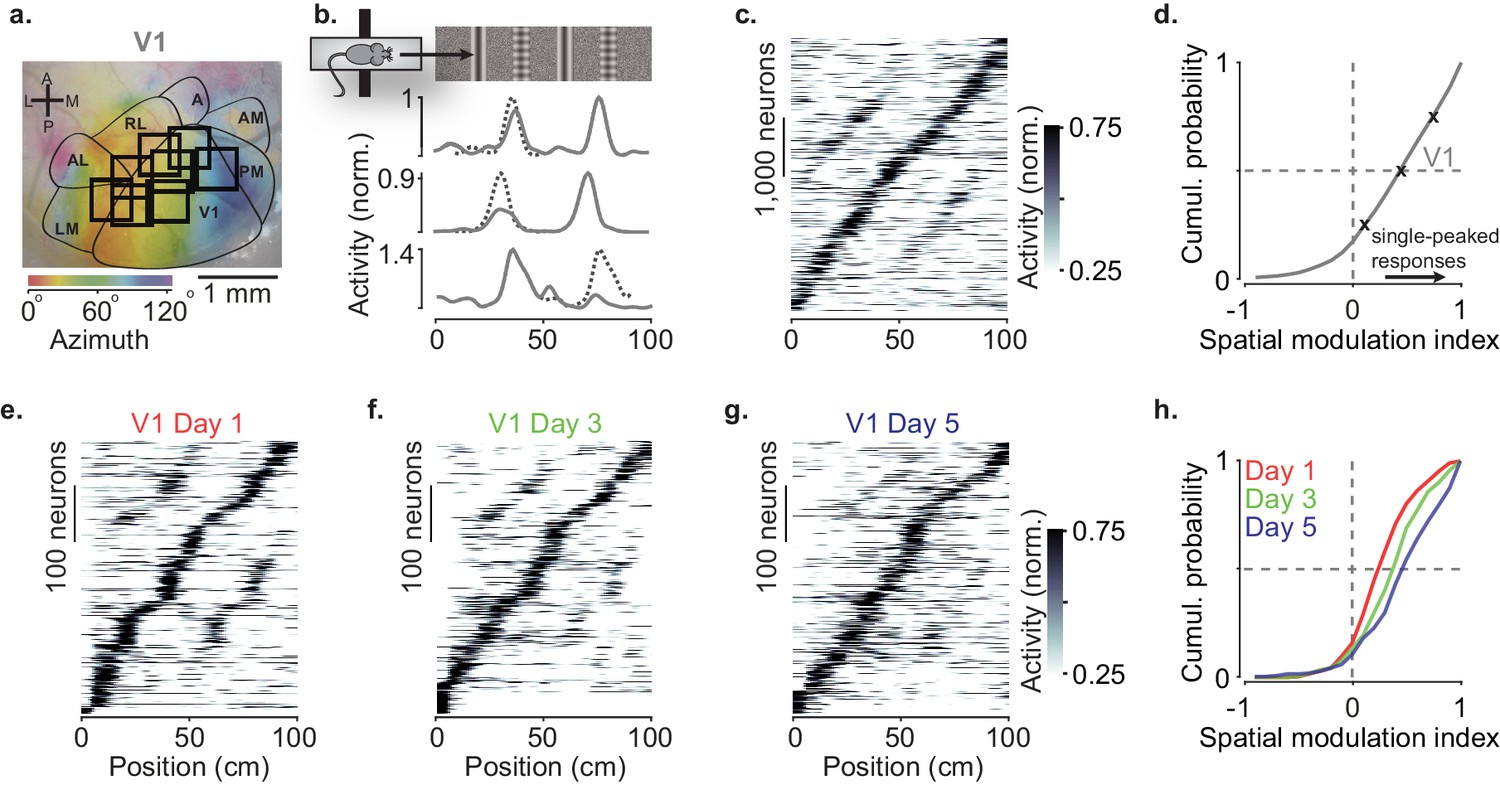
Spatial modulation strengthens with experience.
(a) Example retinotopic map (colors) showing borders between visual areas (contours) and imaging sessions targeting V1 fully or partly (squares, field of view: 500 × 500 µm). (b) Normalized responses of three example V1 neurons, as a function of position in the virtual corridor. The corridor had two landmarks that repeated after 40 cm, creating visually matching segments (top). Dotted lines are predictions assuming identical responses in the two segments. (c) Responses of 4602 V1 neurons (out of 16,238) whose activity was modulated along the corridor (≥5% explained variance), ordered by the position of their peak response. The ordering was based on separate data (odd-numbered trials). (d) Cumulative distribution of the spatial modulation index (SMI) for the V1 neurons. Only neurons responding within the visually matching segments are included (2992/4602). Crosses mark the 25th, 50th, and 75th percentiles and indicate the three example cells in (b). (e–g) Response profiles obtained from the same field of view in V1 across the first days of experience of the virtual corridor (days 1, 3, and 5 are shown) in two mice. (h) Cumulative distribution of SMI for those 3 days, showing median SMI growing from 0.24 to 0.38 to 0.45 across days.
Figure 1—figure supplement 1
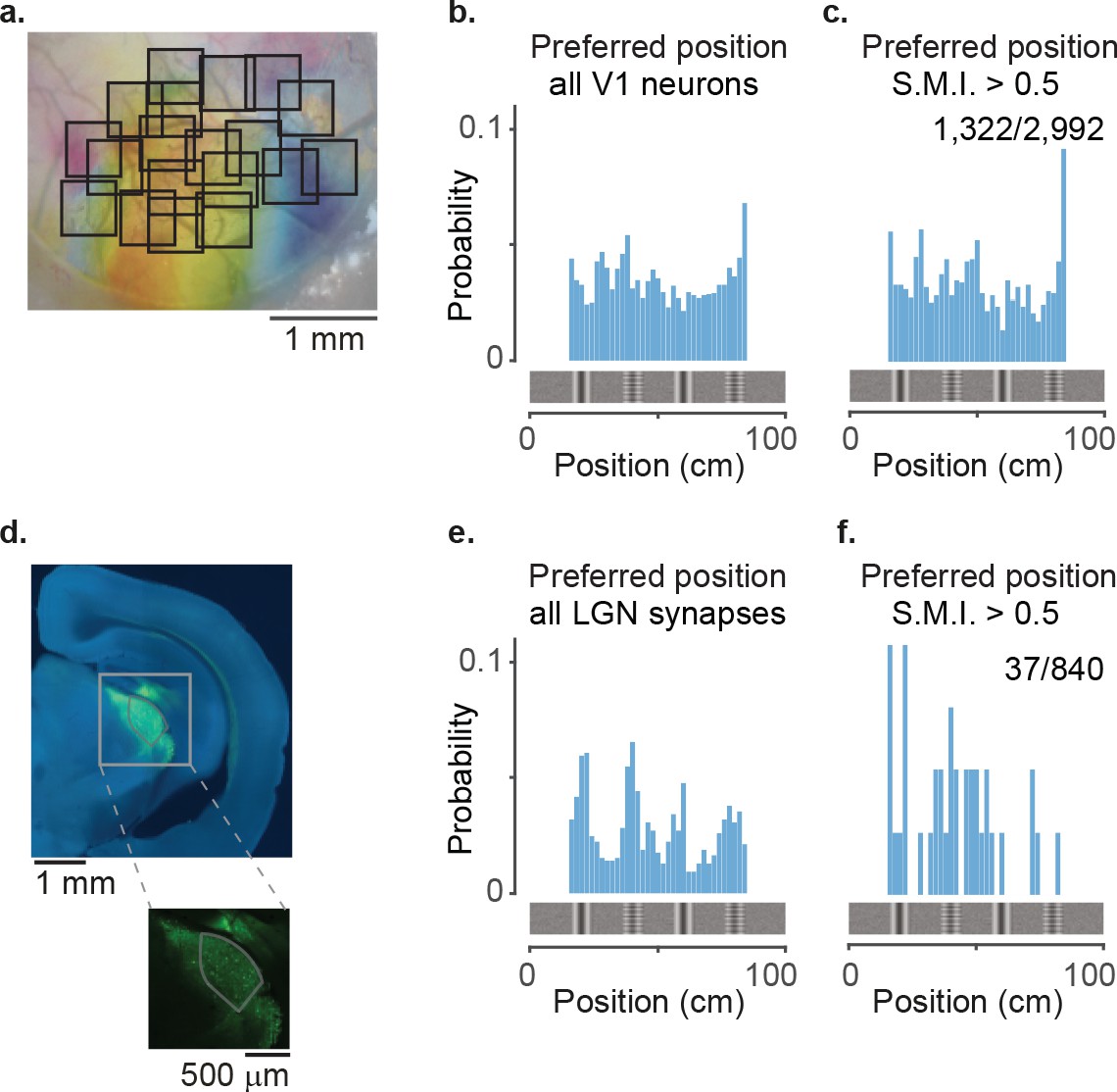
Lateral geniculate nucleus (LGN) boutons tile up the virtual corridor differently from V1 neurons.
(a) Two-photon imaging of cell bodies in visual cortex layer 2/3 across multiple days: example retinotopic map with single-session fields of view (black squares). Combination of Figure 1a and Figure 2e. (b) Distribution along the corridor of preferred positions within the visually matching segments for all V1 neurons (bin size: 2 cm). (c) Same as in (b) for V1 neurons with S.M.I. >0.5 (n = 1322/2992). (d) Example image showing viral expression of GCaMP (green) in the visual thalamus of the right hemisphere (stained with Nissl in blue). Inset: zoomed-in image showing GCaMP expression in LGN and the surrounding nuclei. (e) Distribution of preferred positions along the corridor within the visually matching segments for all 840 LGN boutons (bin size: 2 cm). (f) Same as in (e) for LGN boutons with spatial modulation index (SMI) >0.5 (n = 37/840).
Figure 2 with 1 supplement
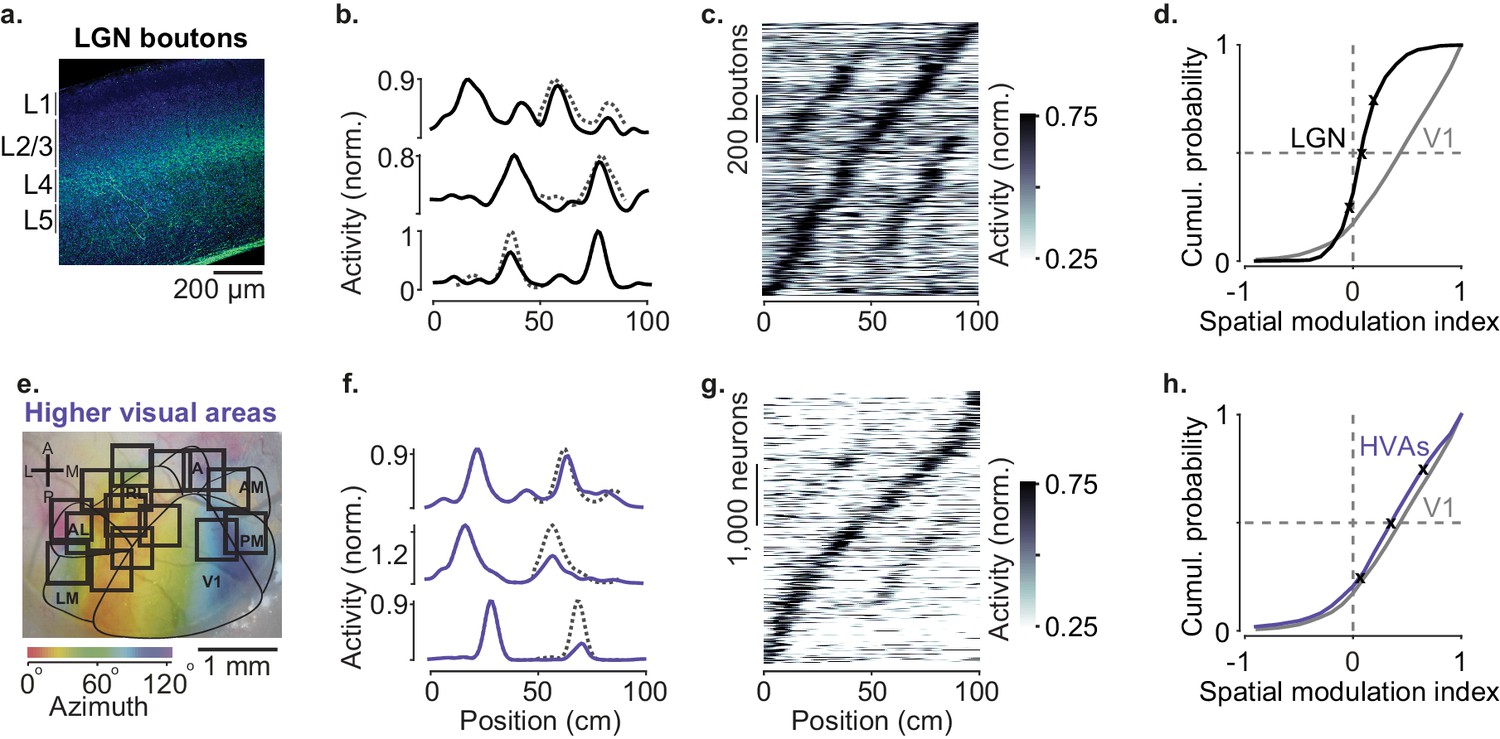
Modulation of visual responses along the visual pathway during navigation.
(a) Confocal image of lateral geniculate nucleus (LGN) boutons expressing GCaMP (GFP; green) among V1 neurons (Nissl stain; blue). GCaMP expression is densest in layer 4 (L4). (b) Normalized activity of three example LGN boutons, as a function of position in the virtual corridor. Dotted lines are predictions assuming identical responses in the two segments. (c) Activities of 1140 LGN boutons (out of 3182) whose activity was modulated along the corridor (≥5% explained variance), ordered by the position of their peak response. The ordering was based on separate data (odd-numbered trials). (d). Cumulative distribution of the spatial modulation index (SMI) for the LGN boutons. Only boutons responding within the visually matching segments are included (LGN: 840/1140). Crosses mark the 25th, 50th, and 75th percentiles and indicate the three example cells in (b). (e) Same as in Figure 1a, showing imaging sessions targeting six higher visual areas (HVA) fully or partly. (f–h) Same as (b–d), showing response profiles of HVA neurons ((g) 4381 of 18,142 HVA neurons; (h) 2453 of those neurons).
Figure 2—figure supplement 1
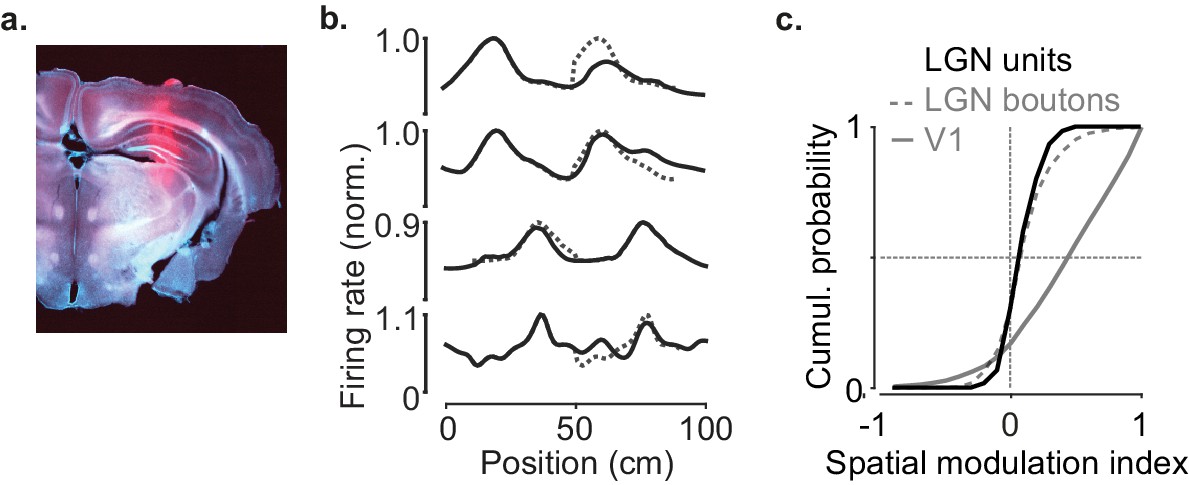
Lateral geniculate nucleus (LGN) boutons and units give similar responses.
(a) Example reconstructed electrode tracks terminating in LGN (red: DiI; brain image stained with DAPI). (b) Response profile patterns of example LGN units recorded using extracellular multi-electrode arrays. Responses are from even trials, ordered, and normalized from odd trials. Dotted lines are predictions assuming identical responses in the two segments. (c) Cumulative distribution of the spatial modulation index in even trials for LGN units (black), LGN boutons (dotted gray line, similar to Figure 2d), and V1 (gray line, similar to Figure 1d) (79 units from two animals).
Figure 3 with 3 supplements
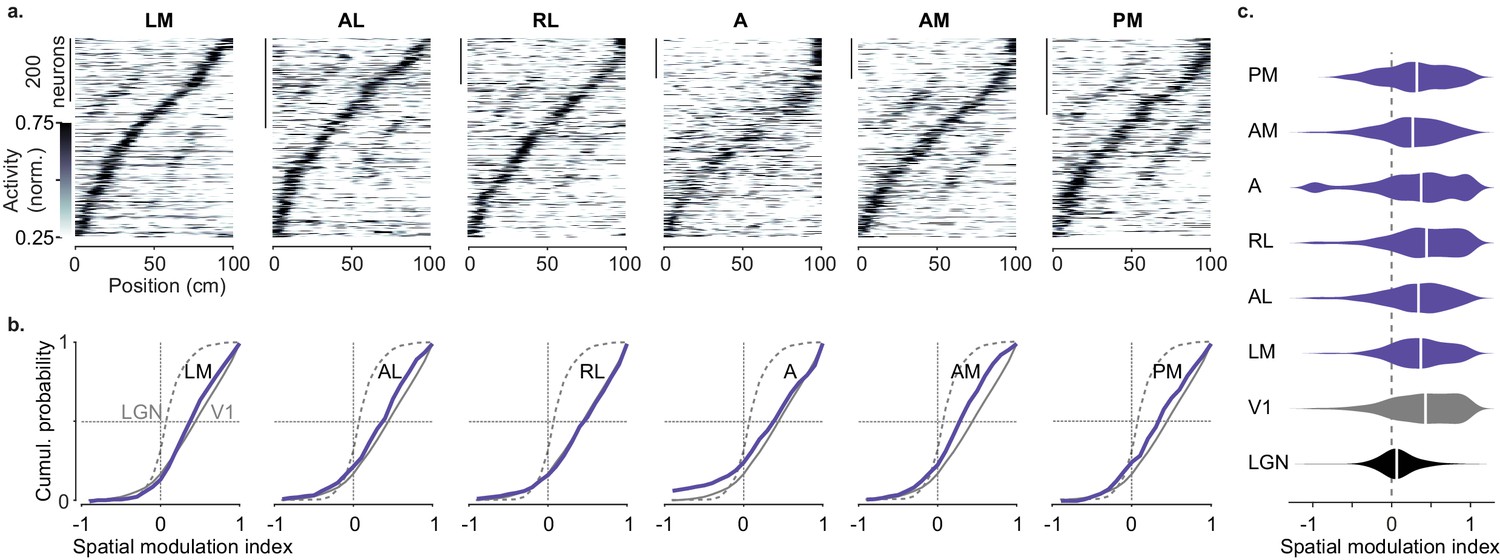
Spatial modulation of individual higher visual areas (HVAs).
(a) Response profile patterns obtained from even trials (ordered and normalized based on odd trials) for six visual areas. Only response profiles with variance explained ≥5% are included (LM: 629/1503 AL: 443/1774 RL: 866/5192 A: 997/4126 AM: 982/3278 PM: 519/2509). (b). Cumulative distribution of the spatial modulation index in even trials for each HVA (purple). Dotted line: lateral geniculate nucleus (LGN; same as in Figure 2d), Gray: V1 (same as in Figure 1d). (c). Violin plots showing the spatial modulation index (SMI) distribution and median SMI (white vertical line) for each visual area (median ± m.a.d. LGN: 0.07 ± 0.11; V1: 0.43 ± 0.31; LM: 0.37 ± 0.25; AL: 0.34 ± 0.28; RL: 0.44 ± 0.31; A: 0.37 ± 0.34; AM: 0.27 ± 0.26; PM: 0.32 ± 0.32).
Figure 3—figure supplement 1
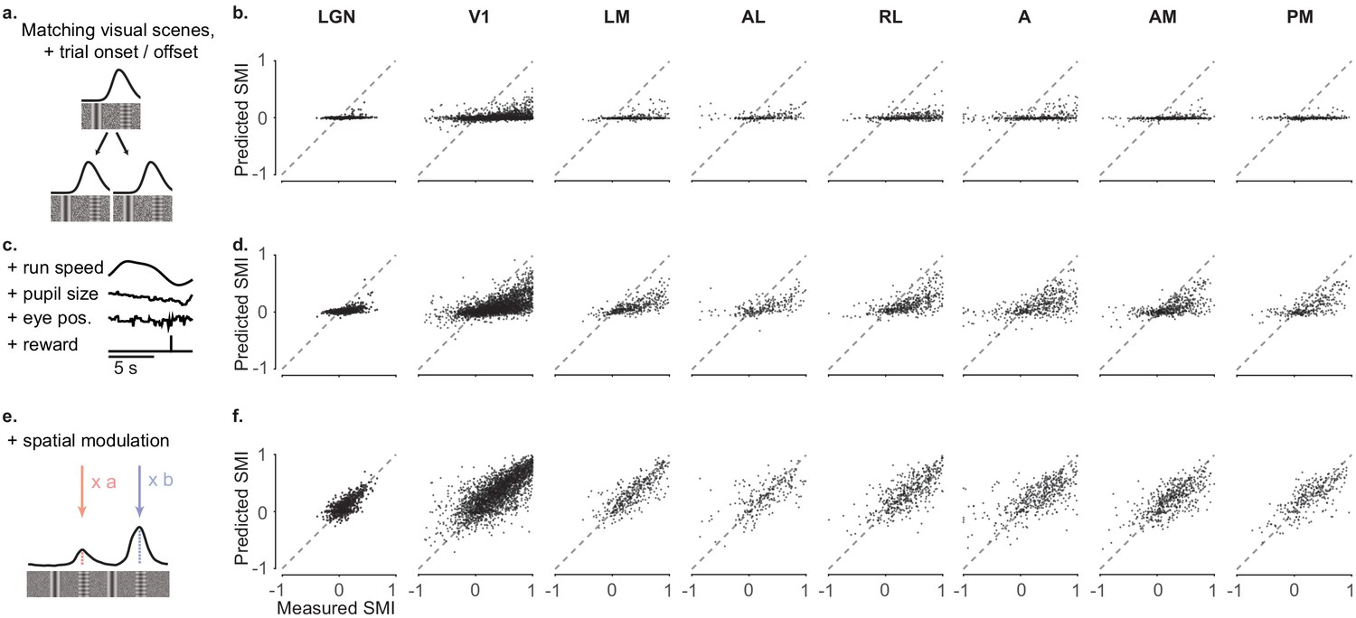
Spatial modulation is not explained by other behavioral and visual factors.
We constructed three models to predict the activity of individual neurons from successively larger sets of predictor variables (Saleem et al., 2018) (a, b) Measured spatial modulation index (SMI) for each visual area versus predictions of the simplest model (‘purely visual model’). The ‘purely visual model’ considers only the repetitions of the visual scenes, trial onset and offset, and as expected, fails to predict the SMIs estimated from the data. Each point represents a neuron. (c, d) Measured SMI for each cortical visual area versus predictions of the ‘non-spatial’ model. The ‘non-spatial’ model also includes the contribution by behavioral factors that can differ within and across trials: speed, reward times, pupil size, and eye position. Adding these factors improves predictions compared to the ‘purely visual’ model but fails to match the measured SMIs. Therefore, the joint contribution of all task-related and visual factors is not sufficient to explain the observed spatial modulation (e, f) Measured SMI for each visual area versus predictions of the ‘spatial’ model. The spatial model allows the peaks in the visually matching segments to vary independently. It provides a much better match to the data.
Figure 3—figure supplement 2
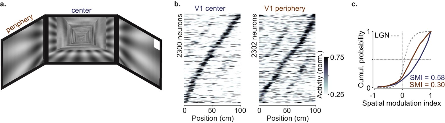
Neurons with central receptive fields showed stronger spatial modulation than neurons with peripheral receptive fields due to the layout of the visual scenes.
(a) Cartoon of the virtual reality scenes layout. (b) Response profile patterns obtained from even trials (ordered and normalized based on odd trials) for portions of V1 with average receptive fields in the center (‘V1 center’;<40° azimuth angle; left) or in the periphery (‘V1 periphery’; right). (c) Cumulative distribution of the spatial modulation index in even trials for ‘V1 center’ (purple) or ‘V1 periphery’ (orange); dotted line: Distribution of lateral geniculate nucleus (LGN) boutons (same as in Figure 2d).
Figure 3—figure supplement 3
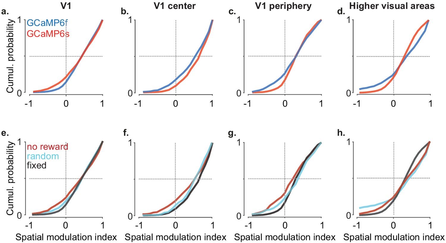
Spatial modulation does not depend on reward or mouse line.
(a) Cumulative distribution of the spatial modulation index (SMI) in even trials for V1 split by Ca2+ indicator, GCaMP6f or GCaMP6s (median ± m.a.d. of SMI: 0.43 ± 0.34 vs. 0.43 ± 0.29). (b) As in (a) for V1 neurons with central receptive fields (median SMI: 0.53 ± 0.31 vs 0.64 ± 0.25). (c) As in (a) for V1 neurons with peripheral receptive fields (median SMI: 0.31 ± 0.31 vs. 0.29 ± 0.24). (d) As in (a) for all higher visual areas (HVAs) combined (median SMI: 0.40 ± 0.37 vs. 0.34 ± 0.24). (e) Cumulative distribution of the SMI in even trials for V1 split by reward condition, no reward, fixed reward at the end of corridor, and reward delivered at random locations (median ± m.a.d. of SMI: 0.42 ± 0.37, 0.43 ± 0.29, 0.44 ± 0.30 respectively). (f) As in (e) for ‘V1 center’ (median SMI: 0.53 ± 0.34, 0.63 ± 0.25, 0.52 ± 0.25;). (g) As in (e) for ‘V1 periphery’ (median SMI: 0.20 ± 0.34, 0.29 ± 0.24, 0.36 ± 0.29). (h) As in (e) for all HVAs (median SMI: 0.33 ± 0.40, 0.35 ± 0.24, 0.48 ± 0.27).
Figure 4 with 1 supplement
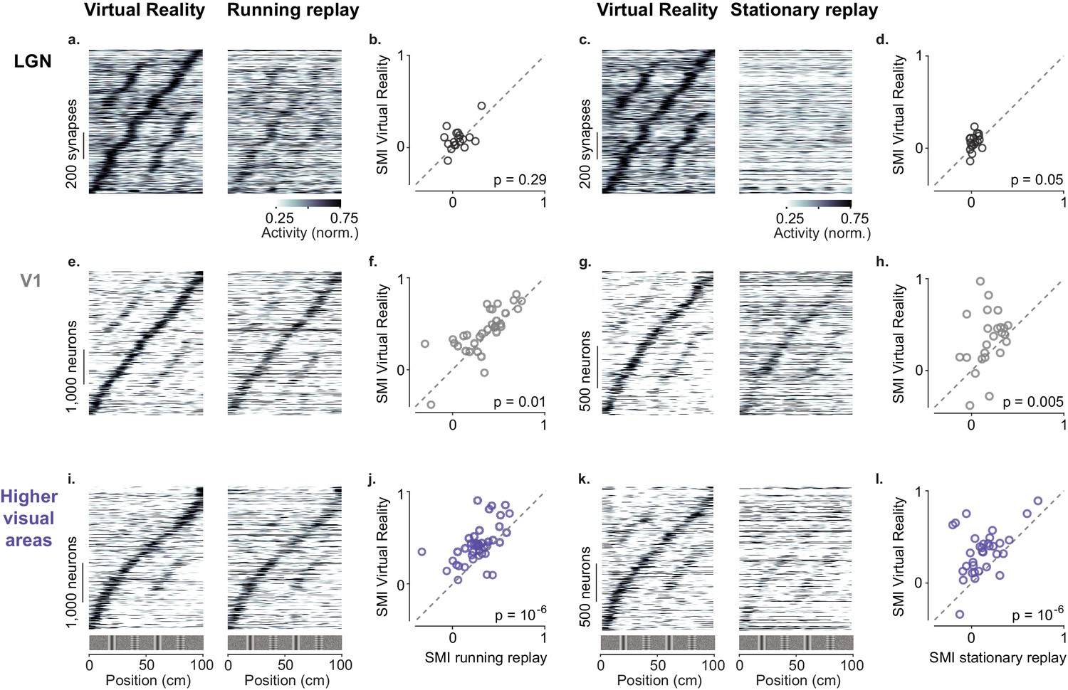
Active navigation enhances modulation by spatial position in visual cortical areas.
(a) Response profiles of lateral geniculate nucleus (LGN) boutons in virtual reality (VR; left) that also met the conditions for running replay (right; at least 10 running trials per recording session), estimated as in Figure 1c. Response profiles of LGN boutons during running replay were ordered by the position of their maximum response estimated from odd trials in VR (same order and normalization as in left panel). (b) Median spatial modulation index (SMI) per recording session in VR versus running replay for LGN (each circle corresponds to a single session; p-values from Wilcoxon signed rank test). (c, d) Same as (a, b) for stationary replay. (e–h). Same as in (a–d) for V1 neurons. (i–l) Same as in (a–d) for neurons in higher visual areas.
Figure 4—figure supplement 1
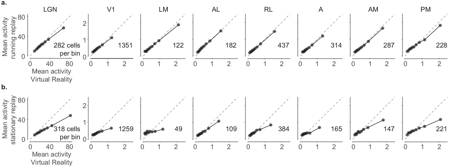
Comparison of neuronal activity in virtual reality (VR) and replay conditions.
(a) Comparison of the mean activity between VR and running replay for all probed visual areas, split into 10 percentile bins. (b) Same as in (a) for stationary replay. Mean activity was similar between VR and running replay but decreased significantly during stationary replay in many areas (paired-sample right-tailed t-test: running replay: lateral geniculate nucleus (LGN): p=0.003; p>0.05 in all cortical areas; stationary replay: LGN: 10−65, V1: 10−24, LM: 0.93, AL: 0.15, RL: 0.06, A: 0.56, AM: 0.03, PM: 10−09).
Tables
Key resources table
| Reagent type (species) or resource | Designation | Source or reference | Identifiers | Additional information |
|---|---|---|---|---|
| Strain, strain background (Mus musculus) | WT, C57BL/6J | Jackson Labs | RRID:IMSR_JAX:000664 | |
| Strain, strain background (Mus musculus) | Ai93, C57BL/6J | Jackson Labs; Madisen et al., 2015 | B6;129S6-Igs7tm93.1(tetO-GCaMP6f)Hze/J RRID:IMSR_JAX:024103 | |
| Strain, strain background (Mus musculus) | Emx1-Cre, C57BL/6J | Jackson Labs; Madisen et al., 2015 | B6.129S2-Emx1(tm1(cre))Krj/J RRID:IMSR_JAX:005628 | |
| Strain, strain background (Mus musculus) | Camk2a-tTA, C57BL/6J | Jackson Labs | B6.Cg-Tg(Camk2a-tTA) 1Mmay/DboJ RRID:IMSR_JAX:007004 | |
| Strain, strain background (Mus musculus) | tetO-G6s, C57BL/6J | Jackson Labs; Wekselblatt et al., 2016 | B6;DBA-Tg(tetO-GCaMP6s) 2Niell/J RRID:IMSR_JAX:024742 | |
| Recombinant DNA reagent | AAV9.CamkII. GCamp6f.WPRE.SV40 | Addgene | Catalogue #: 100834-AAV9 | |
| Software, algorithm | Suite2p | Pachitariu et al., 2016a; https://github.com/cortex-lab/Suite2P | RRID:SCR_016434 | |
| Software, algorithm | KiloSort | Pachitariu et al., 2016b; https://github.com/cortex-lab/Kilosort | RRID:SCR_016422 |
Additional files
Download links
A two-part list of links to download the article, or parts of the article, in various formats.
Downloads (link to download the article as PDF)
Open citations (links to open the citations from this article in various online reference manager services)
Cite this article (links to download the citations from this article in formats compatible with various reference manager tools)
Spatial modulation of visual responses arises in cortex with active navigation
eLife 10:e63705.
https://doi.org/10.7554/eLife.63705


