Inhibitory control of frontal metastability sets the temporal signature of cognition
- Univ Lyon, Université Lyon 1, Inserm, Stem Cell and Brain Research Institute U1208, France
- Sorbonne Université, CNRS, Institut des Systèmes Intelligents et de Robotique, ISIR, F-75005, France
- Nash Family Department of Neuroscience and Friedman Brain Institute, Icahn School of Medicine at Mount Sinai, United States
Figures
Figure 1
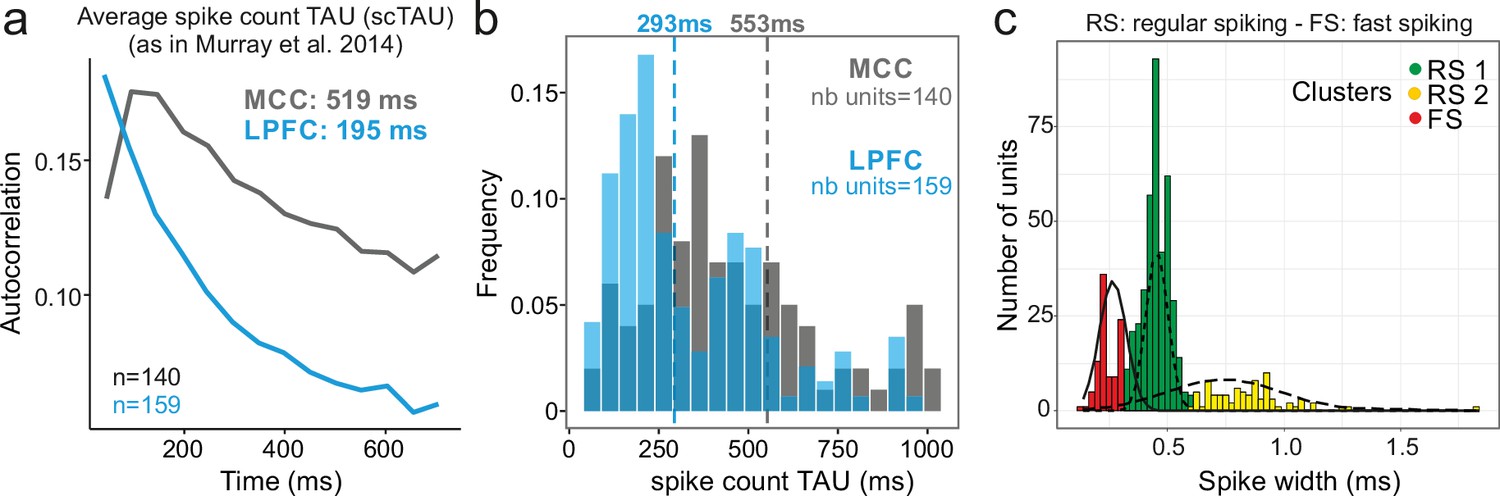
Midcingulate cortex (MCC) and lateral prefrontal cortex (LPFC) spike count autocorrelograms.
(a) Population exponential fit. Autocorrelograms were computed for each unit and the fit was performed on all the units of the MCC (dark grey) and the LPFC (blue) to extract the decay parameter scTAU (as in Murray et al., 2014). (b) Single unit fits were used to capture individual spiking timescales and produce the distribution of scTAU values for each region. Dotted lines represent the median of scTAU. (c) Clustering of spike shape. After extracting the spike width and amplitude from each unit average waveform, we performed a hierarchical clustering revealing the presence of three groups of units (coloured groups RS1, RS2, FS; see Materials and methods). Fitting Gaussian mixed model on the population (lines) confirmed the presence of the three clusters. In the paper, units with narrow spike width were termed as fast spiking (FS), whereas units with broader waveform were marked as regular spiking (RS: RS1 + RS2).
Figure 2 with 3 supplements
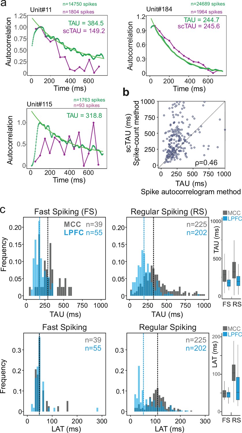
Spike autocorrelogram and temporal signatures in midcingulate cortex (MCC) and lateral prefrontal cortex (LPFC).
(a) Three single examples of spike count (purple, scTAU) vs. normalized spike autocorrelograms (green) contrasting the outcome of the two methods. The measured time constant (TAU) is indicated for both when possible. Numbers of spikes used for each method is also indicated. (b) TAU values extracted from each methods are significantly correlated (n=280, Spearman’s rho(282) = 0.46, p<10–15). (c) Distributions of TAUs (upper histograms) and peak latencies (LAT – lower histogram) for fast spiking (FS) (left) and regular spiking (RS) (right) units. ‘n’ indicates the number of units. Vertical dashed lines indicate medians of respective populations. Boxplots on the right show the respective population data. TAU values were longer in MCC (dark grey) than in LPFC (blue) for both FS and RS (linear model fit on BLOM transformed TAU for normality, TAU = region * unit type, region: t=−4.68, p<10–6, unit type: ns, interaction: ns). Peak latencies significantly differed between MCC and LPFC for RS but not for FS units (medians: MCC FS = 48.5 ms, RS = 102.0 ms, LPFC FS = 48.5 ms, RS = 51.8 ms; linear model fit on BLOM transformed latency for normality, latency = region * unit type, interaction: t-value=−3.57, p<10–3).
Figure 2—figure supplement 1
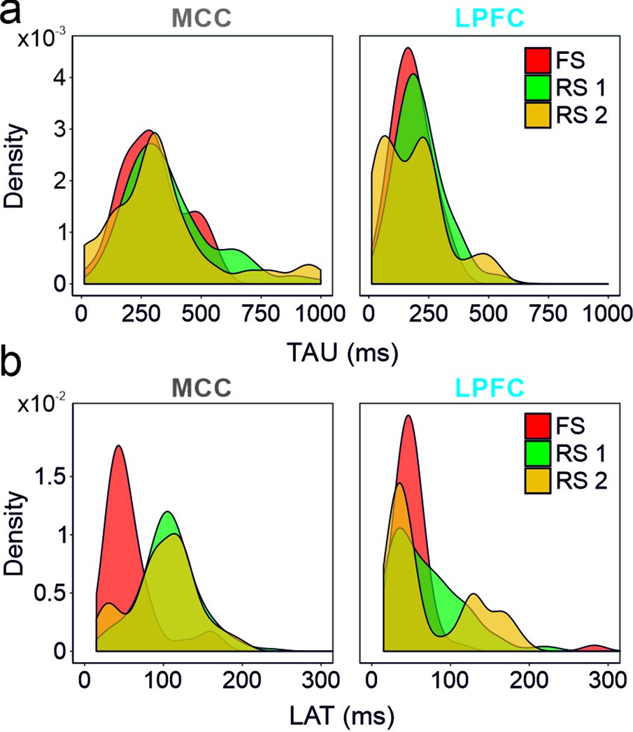
Spike autocorrelogram features considering the three clusters of populations (fast spiking [FS], regular spiking 1 [RS1] and RS2) in the midcingulate cortex (MCC) and lateral prefrontal cortex (LPFC).
(a) TAUs and (b) autocorrelogram peak latencies distribution in the three-cell populations in the MCC and the LPFC. Densities were computed using a Gaussian kernel with standard deviation of 50 and 15 ms respectively for TAU and peak latencies.
Figure 2—figure supplement 2
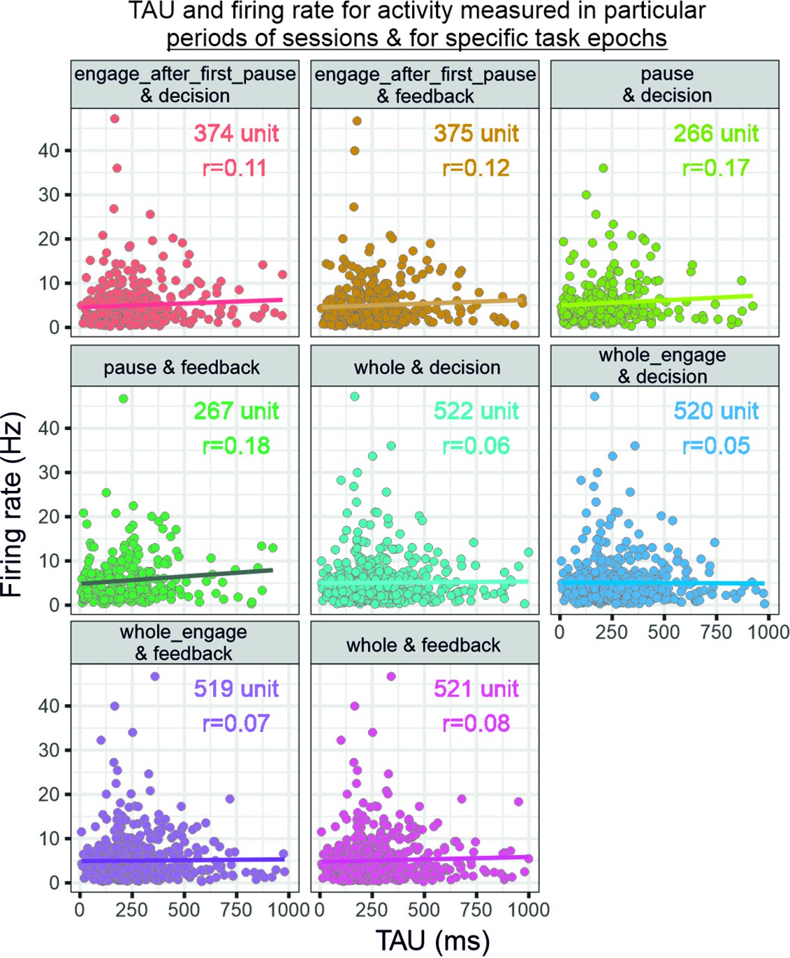
Relationship between firing rate and temporal signatures.
The graphs relate TAU measured from specific recording periods (whole, engage, pause, etc.) and firing rate as measured in specific task epochs (feedback or decision). Note that each selection of period for firing rate measures changes the number of units that can be analysed because of the criteria on data size (see figure). Spearman’s rank correlations with Bonferroni corrected p-values (eight comparisons): engage after first pause and decision: rho(374)=0.11, p=0.31; engage after first pause and feedback: rho(375)=0.12, p=0.13; pause and decision: rho(266)=0.17, p=0.042; pause and feedback: rho(267)=0.18, p=0.031; whole and decision: rho(522)=0.06, p=1.00; whole engage and decision: rho(520)=0.05, p=1.00; whole engage and feedback: rho(519)=0.07, p=1.00; whole and feedback: rho(521)=0.08, p=0.54.
Figure 2—figure supplement 3
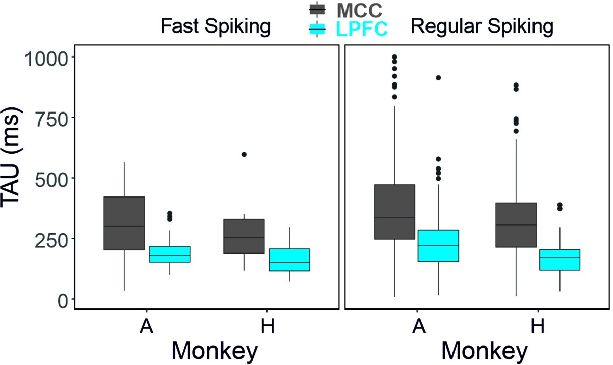
Average TAU for each cell type, area, and for each animal separately.
Sample sizes: monkey A: LPFC FS n=31, RS n=142; MCC FS n=31, RS n=163 - for monkey H: LPFC FS n=26, RS n=73 ; MCC FS n=10, RS n=94.
Figure 3
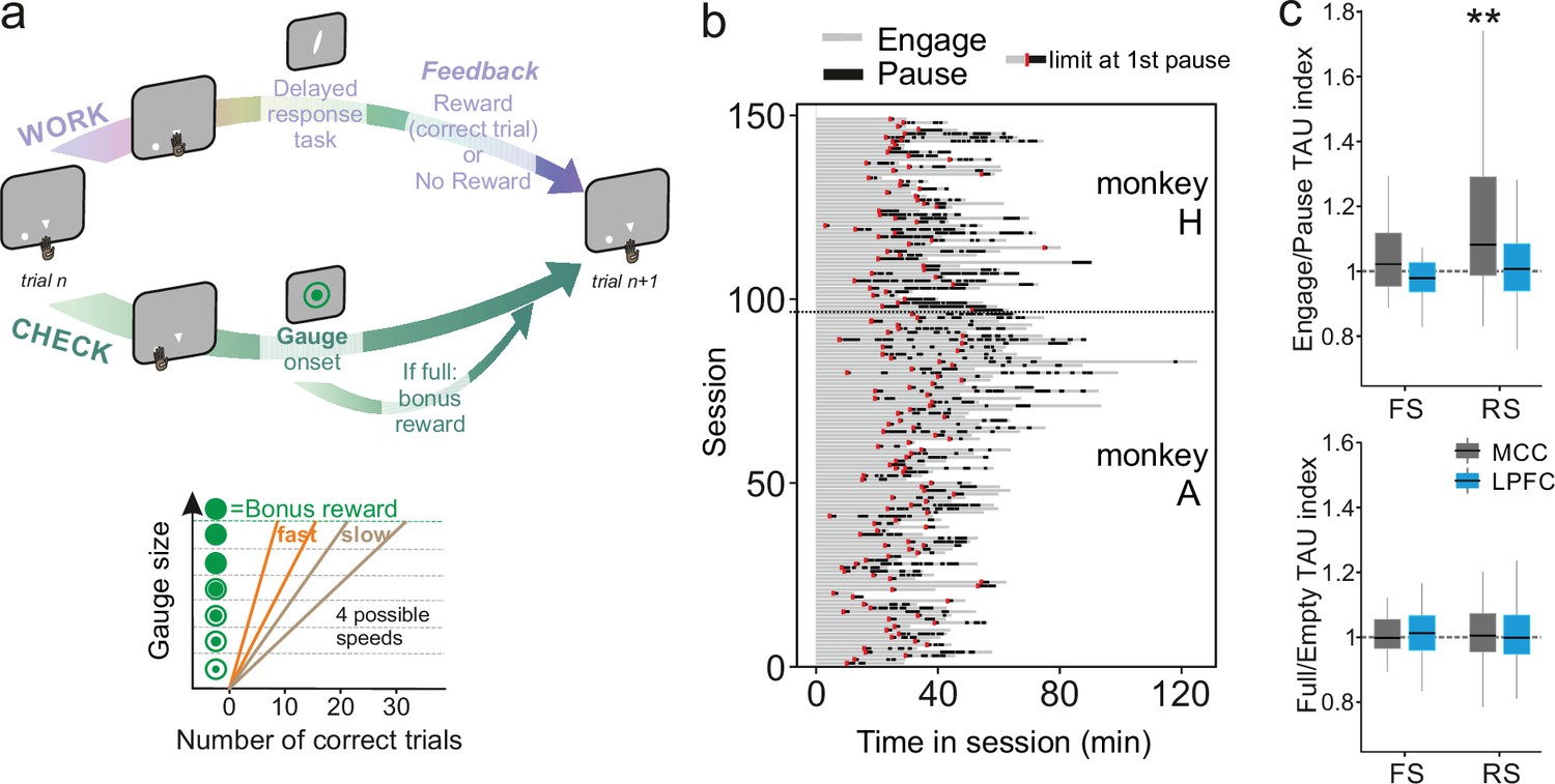
Behavioural engagement in task and spiking timescale changes.
(a) Schematic representation of the task. At the start of each trial, animals can either initiate a delayed response task (WORK option) which can lead to one reward delivery, or use the CHECK option to check the current size of the gauge (or collect the bonus reward). Each reward in the task contributes to increase the gauge size and bring the bonus availability closer. The graph (bottom) schematized the speed of increase of the gauge size which varies between blocks (fast or slow blocks). (b) Distribution of pauses in sessions. Each line represents the time course of behaviour for one session for monkey H and monkey A. Grey zones represent engagement in the task, black zones represent pauses in work. Red marks indicate the start limit of the first pause in session which defined the beginning of the period taken for control analyses. (c) Boxplots of indices for each unit type and region calculated to estimate potential changes in TAU between engage and pause (top), and between empty and full gauge (bottom). TAUs increased in engage vs. pause only for midcingulate cortex (MCC) regular spiking (RS) units.
Figure 4 with 2 supplements
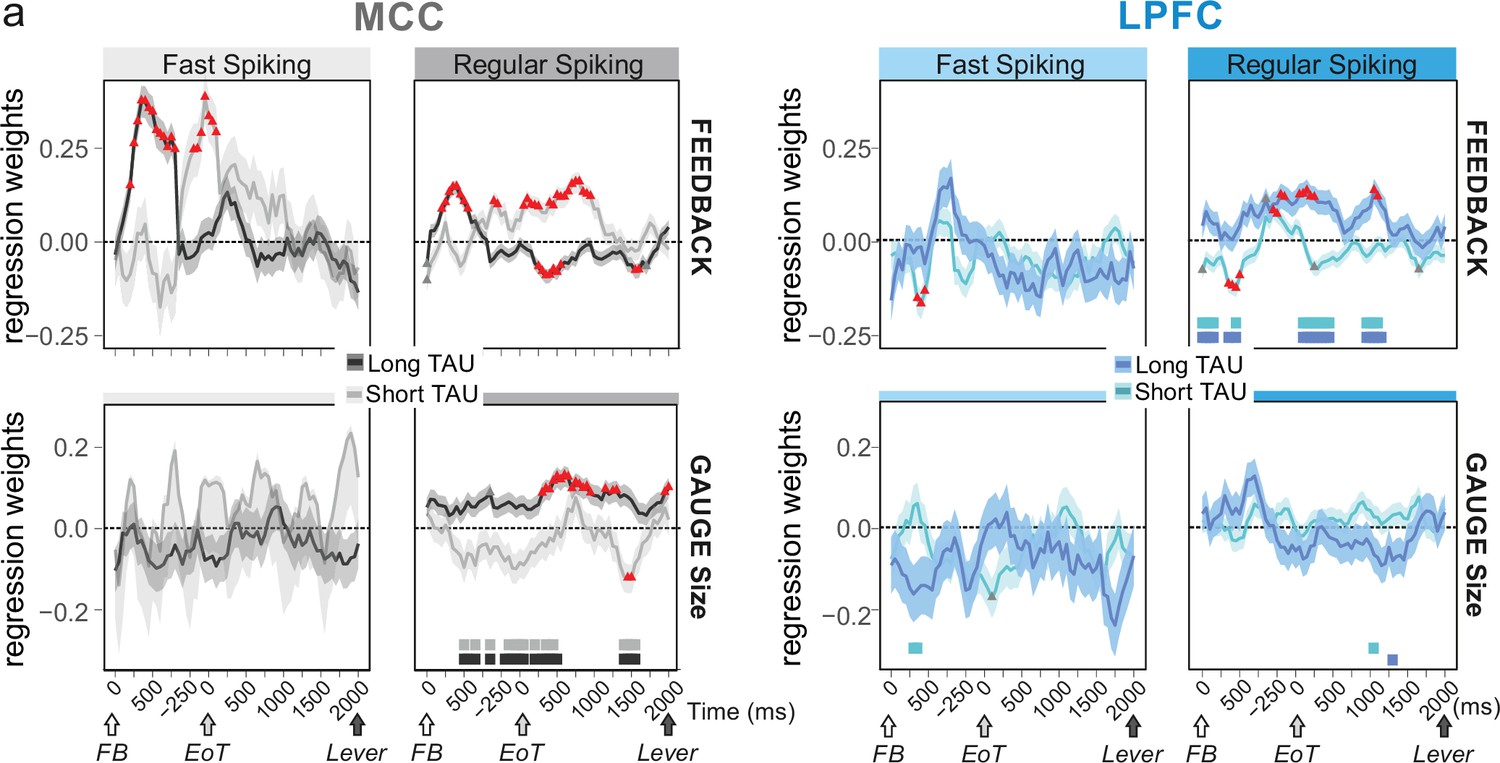
Encoding of feedback and gauge size for different unit types and spiking timescales and rostro-caudal distribution.
(a) Regression weights (β-coefficients) for the midcingulate cortex (MCC) (grey) and lateral prefrontal cortex (LPFC) (blue) unit populations obtained from time-resolved glmm for feedback (reward vs. no reward; top graphs) and gauge size (bottom) (see group analyses using glmm’ in Materials and methods). Regression weights are obtained at successive time points covering the entire intertrial period between feedback onset and the lever onset in the following trial. Significant effects are indicated by a red triangle (p<0.05 corrected) when more than two successive bins are concerned, shadings indicate standard deviations. Positive values depict a population activity bias towards negative feedback (top) and positive slope of linear coding for gauge size (bottom). Data are presented for fast spiking (FS) and regular spiking (RS) units (left and right respectively for each panel) and have been obtained on subpopulations with short or long TAU values (determined by a median split). Short and long TAU populations are represented by light and dark colour intensity, respectively. Thick bars above the x-axes indicate significance of the coloured corresponding data compared to a null distribution generated through permutations of median split unit identity. Note in particular the dissociation for RS MCC units with short and long TAU respectively coding for feedback and gauge size.
Figure 4—figure supplement 1
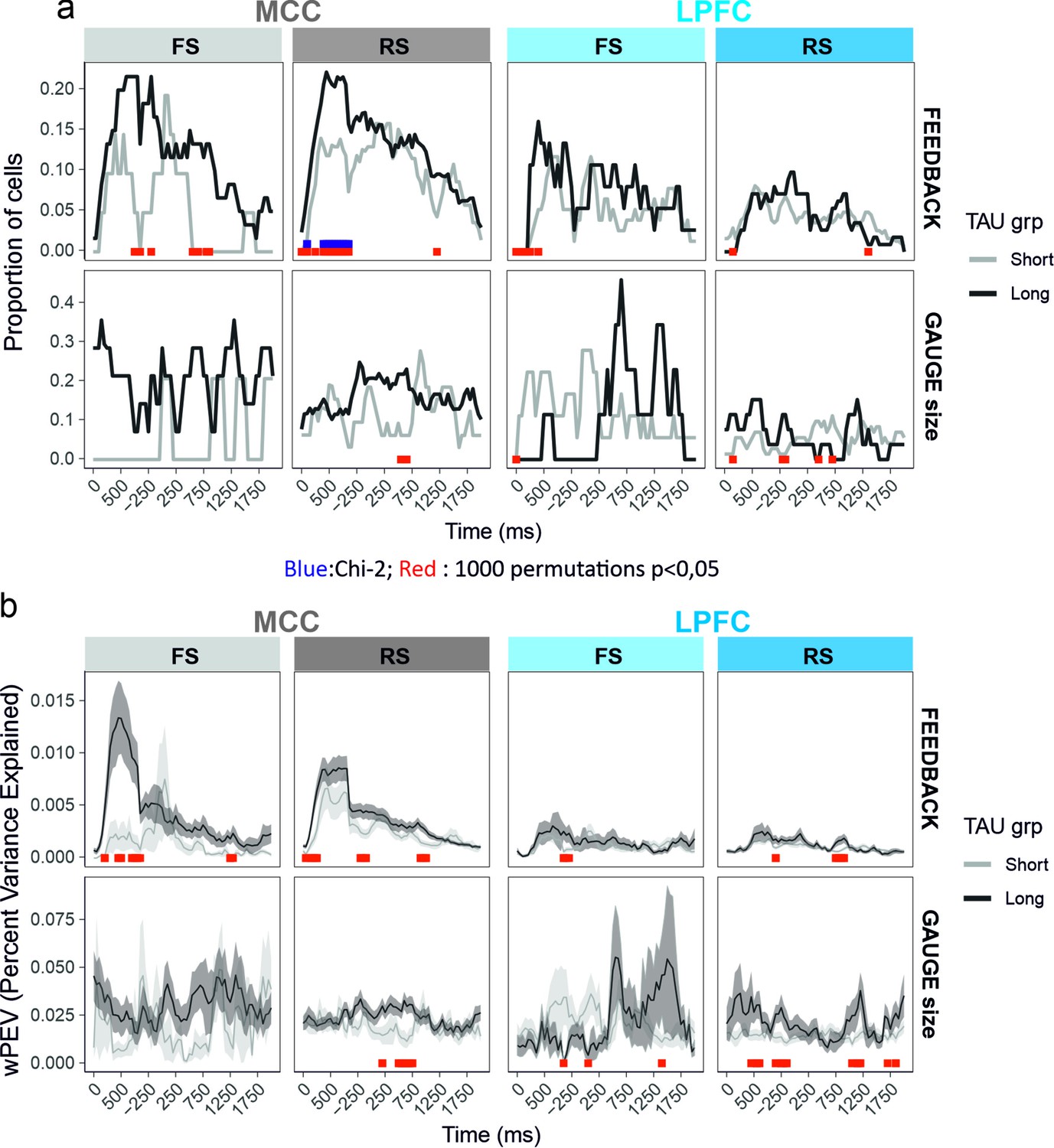
Time-resolved single unit analyses of gauge size and feedback valence encoding between the feedback time (0) and lever onset.
Each single unit activity has been analysed using a glm including feedback, gauge, and decision as fixed effects. The proportion of single units presenting significant variation by each factor at the successive time bins is presented in (a). The average weighted mean proportion of explained variance (wPEV) is presented in (b). Data are shown for the two median split populations based on TAU values computed on the entire session. Red and blue marks on the x axes reflect time bins for which the proportions for the unit populations are not equal (Chi-2, blue in a), and for which values differ from null distribution obtained from 1000 permutations across unit types labels. In red significance results for permutations of TAU labels within cell_type × area to construct two NULL distributions (short and long) to compare the real data to. Permutations of TAU labels hence provide two statistics. For the sake of clarity, red marks of the figure indicate time bins for which at least one of the permutation tests was significant (a=0.05).
Figure 4—figure supplement 2
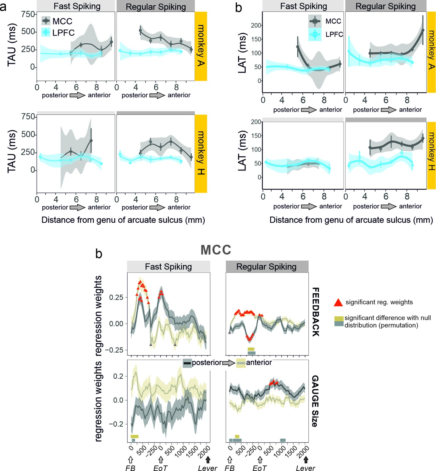
Anatomical heterogeneity of TAU.
(a) Averaged TAU values measured along the postero-anterior axis in the midcingulate cortex (MCC) and lateral prefrontal cortex (LPFC), for both monkeys. (b) Anatomical distribution of LAT in MCC and LPFC for the two monkeys. (c) Regression weights reflecting the coding strength of feedback and gauge size for MCC unit populations separated by their posterior vs. anterior location and unit type (fast spiking vs. regular spiking). Thick bars above the x-axes indicate significance of the corresponding coloured data compared to a null distribution generated through permutations of anatomical unit identity.
Figure 5 with 3 supplements

Temporal signature of LPFCm and MCCm recurrent network biophysical models.
(a) Scheme of the frontal recurrent networks modelled, with 80% excitatory (green) and 20% inhibitory (red) neurons and sparsity of synaptic connections. (b) Membrane potential in the 484 excitatory (lower part) and 121 inhibitory (upper part) neurons of LPFC and MCC example network models (respectively LPFCm and MCCm ; 'm' for model) with parameter set to approximate LPFC dynamics (gCAN = 0.025 mS·cm–2, gAHP = 0.022 mS·cm–2, gGABA-B=0.0035 mS·cm–2; see text and legend of Figure 6b for the choice of LPFCm and MCCm standard gAHP and gGABA-B maximal conductances) and MCC dynamics (gCAN = 0.025 mS·cm–2, gAHP = 0.087 mS·cm–2, gGABA-B=0.0143 mS·cm–2). (c) (Upper left) Membrane potential of an example excitatory neuron of LPFCm. Scaling bars 1 s and 10 mV (spikes truncated). (Lower left) Autocorrelogram of this LPFCm example excitatory neuron (black) and its exponential fit (red, see Materials and methods). (Right) Bivariate probability density distribution of autocorrelogram parameters in LPFCm excitatory neurons. Contour lines at 50%, 75%, and 90% of the maximum of the bivariate probability density distribution in LPFC monkey regular spiking (RS) units. (d) Same as (c) for LPFCm inhibitory neurons, with contour lines from the bivariate probability density distribution in LPFC monkey fast spiking (FS) units. (e,f) Same as (c,d), for the MCCm and MCC.
-
Figure 5—source data 1
Summary of the effects of the main parameters determining TAU and LAT in the network model.
- https://cdn.elifesciences.org/articles/63795/elife-63795-fig5-data1-v2.docx
Figure 5—figure supplement 1
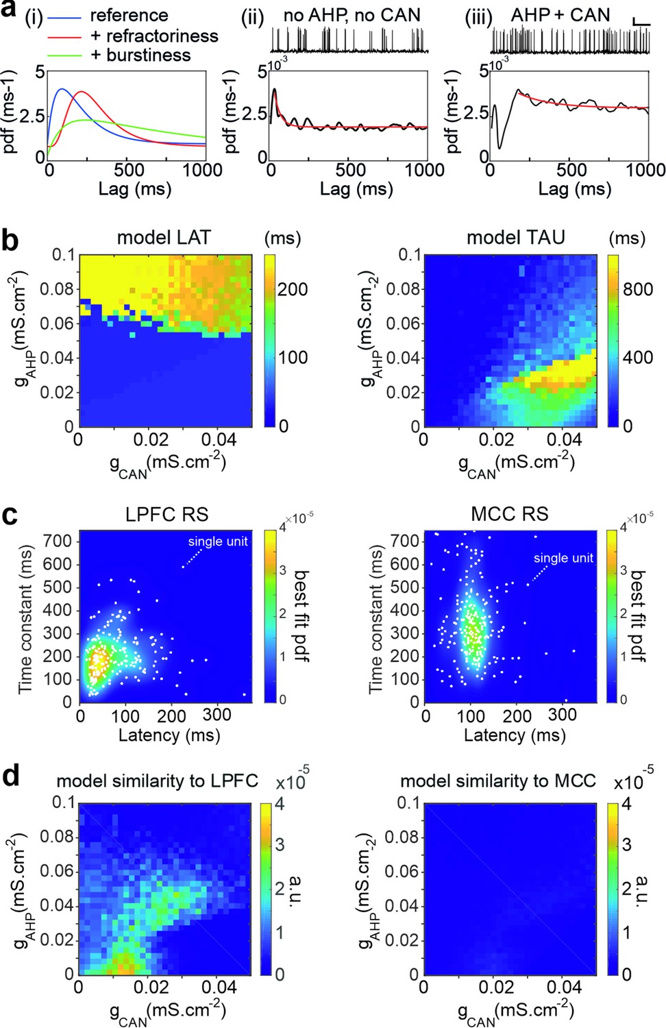
Temporal signature in the pyramidal biophysical neuron model.
(a) In (i) schematic shapes of the autocorrelogram of a neuron (e.g. regular spiking, blue), of the same neuron with a larger refractory period (e.g. due to increased hyperpolarizing ionic conductance, red) or with higher burstiness of the spike discharge (e.g. due to increased depolarizing conductance-mediated positive feedbacks, green). (ii–iii) Autocorrelogram of a model pyramidal neuron (ii) in the absence (gCAN = 0 mS·cm-2, gAHP = 0 mS·cm-2) of CAN or AHP, or (iii) with gCAN = 0.05 mS·cm-2 and gAHP = 0.1 mS·cm-2. Scaling bars 1 s and 25 mV. (b) Maps of the autocorrelogram latency (left) and time constant (right), as a function of gCAN and gAHP maximal conductances. (c) Bivariate probability density distribution of neuronal autocorrelogram LAT and TAU in regular spiking (RS) units in both the lateral prefrontal cortex (LPFC) (left) and midcingulate cortex (MCC) (right) in monkeys (each dot represents an individual unit and the underlying map is the best-fit distribution). (d) Similarity of the temporal signature between the frontal pyramidal neuron model and the population of RS units in the LPFC (left) and MCC (right), as a function of gCAN and gAHP maximal conductances.
Figure 5—figure supplement 2
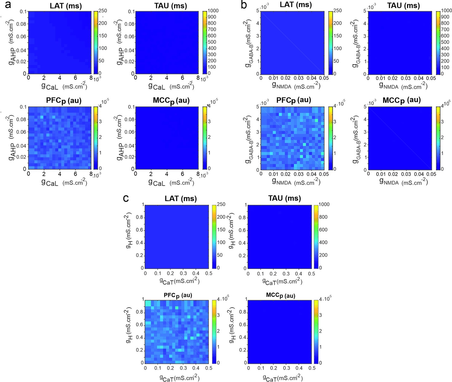
Temporal signature in the pyramidal neuron model as a function of adaptation and rebound intrinsic and slow synaptic conductances.
Maps of LAT (upper left) and TAU (upper right) and of the temporal signature similarity of the pyramidal neuron to regular spiking (RS) neurons of the modelled prefrontal cortex (PFCm) (lower left) and midcingulate cortex (MCCm) (lower right), as a function of (a) the high-threshold calcium and after-hyperpolarization maximal conductances (gCaL and gAHP) that set adaptation properties, (b) the low-threshold calcium (CaT) and hyperpolarization-activated H maximal conductances (gCaT and gH) that set post-inhibitory rebound properties, and (c) the synaptic NMDA and GABA-B maximal conductances (gNMDA, gGABA-B) that set slow synaptic transmission.
Figure 5—figure supplement 3
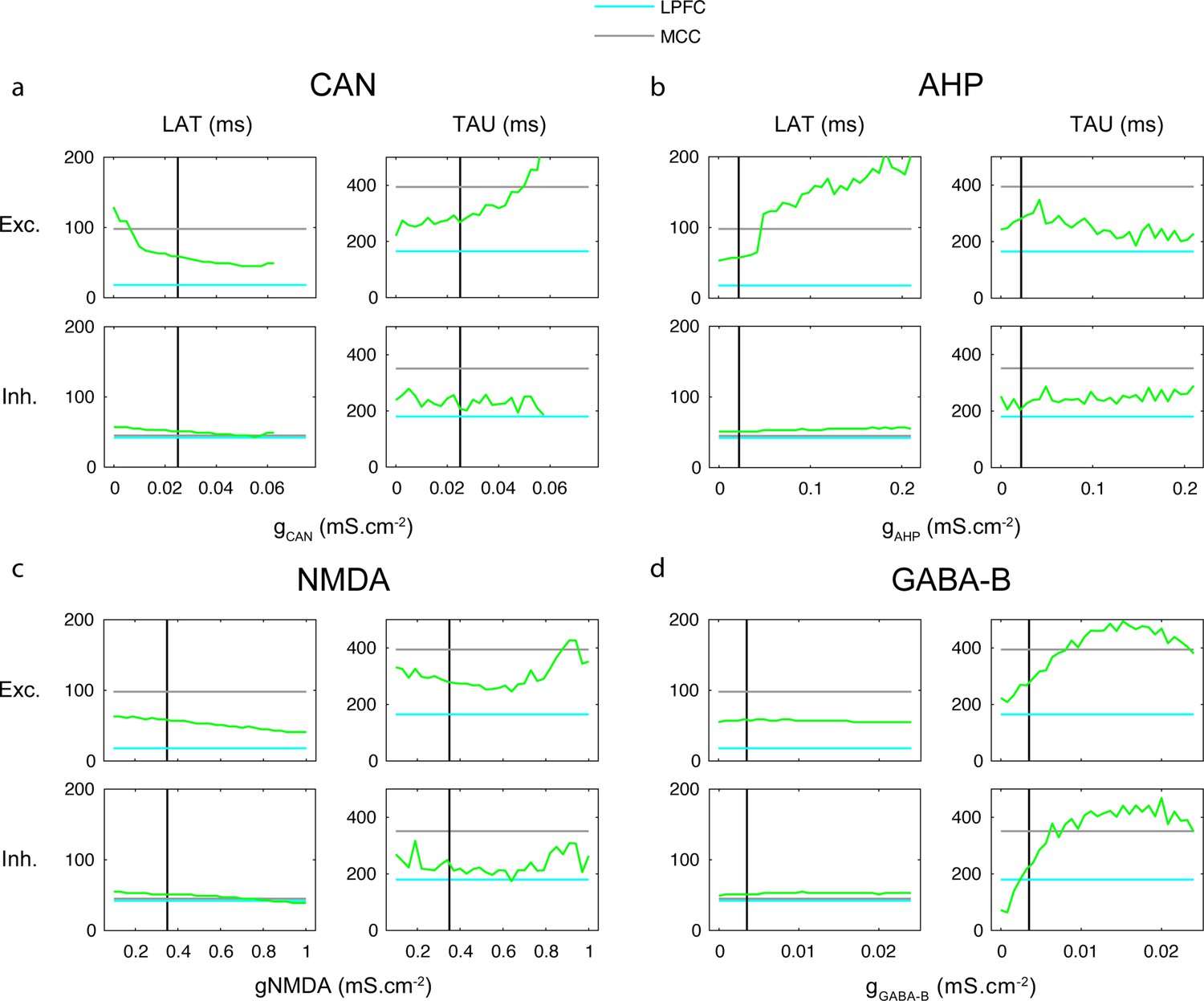
One-dimensional explorations of key parameters determining TAU and LAT in the network model.
LAT (left) and TAU (right) in Exc (upper) and Inh (lower) neurons in the model (green), as a function of the (a) CAN, (b) AHP, (c) NMDA, and (d) GABA-B maximal conductances. The default lateral prefrontal cortex (LPFCm) model parameter value is indicated (vertical black) as well as experimental LAT and TAU in the LPFC (blue) and midcingulate cortex (MCC) (grey).
Figure 6 with 2 supplements
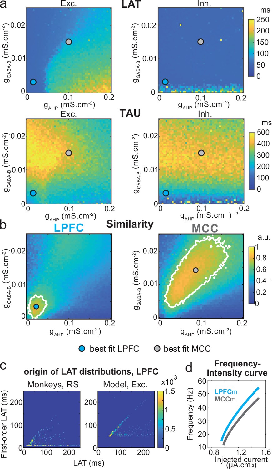
Similarity to monkey lateral prefrontal cortex (LPFC) and midcingulate cortex (MCC) temporal signatures critically depends on AHP and GABAB conductance in the network model.
(a) Mean population LAT (top) and TAU (bottom) in Exc (left) and Inh (right) neurons, as a function of AHP and GABA-B maximal conductances. Blue and grey dots indicate the (gAHP, gGABA-B) parameter values of the best fits for LPFCm and MCCm, respectively. (b) Similarity of the temporal signature between the network model and monkey data in the LPFC (left) and MCC (right), as a function of AHP and GABA-B maximal conductances (see Materials and methods). In (a) and (b), the value for each (gAHP, gGABA-B) is averaged over five simulations. Contour line at 80% of maximum similarity. LPFCm and MCCm (gAHP, gGABA-B) parameter values calculated as coordinates of the contour delimited area’s weighted average. (c) Bivariate probability density distribution of the autocorrelogram LAT and first-order latency (the latency of the inter-spike interval [ISI] distribution) in regular spiking (RS) units in monkey LPFC (left) and excitatory neurons in the example LPFCm (right). The model accounts for two distinct neuronal subsets in RS neurons, where LAT is determined by first-order latency solely (due to gAHP-mediated refractoriness; diagonal band), or in conjunction with other factors (gGABA-B slow dynamics-mediated burstiness and recurrent synaptic weight variability; horizontal band). (d) Single excitatory neuron frequency/intensity relationship in LPFCm (blue) and MCCm (grey) in response to a constant injected current.
Figure 6—figure supplement 1
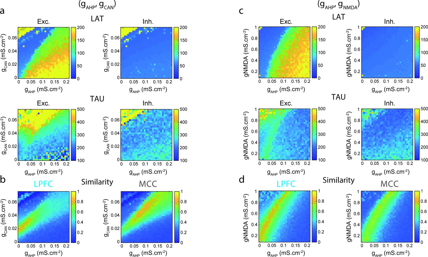
Two-dimensional explorations in (gAHP, gCAN) and (gAHP, gNMDA) spaces.
(a) Mean population LAT (top), TAU (bottom) in Exc (left) and Inh (right) neurons, as a function of AHP and CAN maximal conductances. (b) Similarity of the temporal signature between the network model and monkey data in the lateral prefrontal cortex (LPFC) (left) and midcingulate cortex (MCC) (right), as a function of AHP and CAN maximal conductances (see Materials and methods). (c) Same as (a) and (d) same as (b) as a function of AHP and NMDA maximal conductances.
Figure 6—figure supplement 2
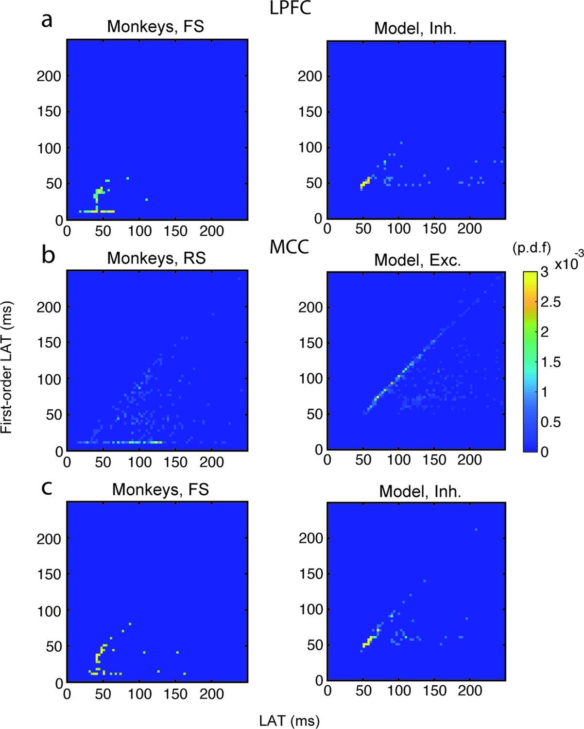
Relationship between autocorrelogram latency and first-order (inter-spike interval [ISI]) latency in lateral prefrontal cortex (LPFC) fast spiking (FS) units/inhibitory (Inh) neurons, and in midcingulate cortex (MCC) regular spiking (RS) units/excitatory (Exc) and MCC FS units/Inh neurons.
Bivariate probability density distribution of the autocorrelogram LAT and first-order latency (i.e. the latency of the ISI distribution) in (a) LPFC monkey FS units (left) and network Inh neurons (right), (b) MCC monkey RS units (left) and network Exc neurons (right), and (c) MCC monkey FS units (left) and network Inh neurons (right).
Figure 7 with 4 supplements
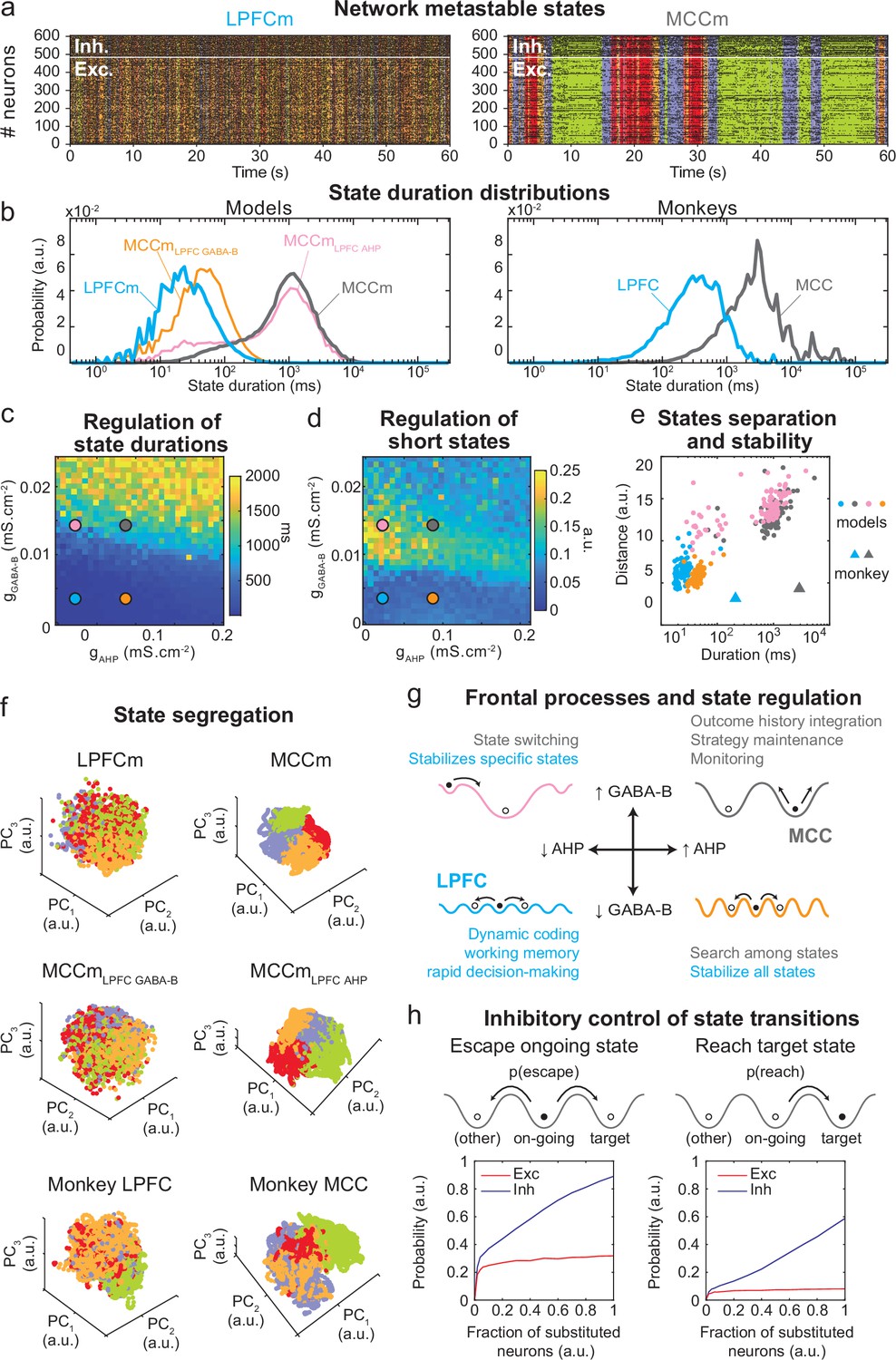
Properties of metastable states in the lateral prefrontal cortex (LPFC) and midcingulate cortex (MCC).
(a) LPFCm and MCCm spiking raster plots (black dots), with Hidden Markov model states (HMM, coloured bands). (b) State duration distributions: probability distributions of being in states of given durations in LPFCm (blue), MCCm (grey), MCCm with LPFCm gAHP (MCCmLPFC AHP pink), and MCCm with LPFCm gGABA-B (MCCmLPFC GABA-B, orange) models (left) and monkey LPFC (blue) and MCC (grey) areas (right). Each model was simulated 100 times and analysed via HMM, while monkey data was analysed via HMM with 100 different initiation parameter states. Periods above 300 s were excluded. (c, d) Regulation of state duration and short states: median state duration (c) and Kolmogorov-Smirnov one-sample test statistic or maximal distance of state duration probability distributions to log-normality, as a measure of the over-representation of short states (d), as a function of gAHP and gGABA-B maximal conductances. Coloured disks indicate parameter values of models LPFCm, MCCm, MCCmLPFC AHP, and MCCmLPFC GABA-B, respectively. Each point is the average of five simulations. (e) Separation between states: average distances between HMM states (averaged pairwise distance between neural centred standardized frequency centroids [temporal averages] of HMM states), as a function of median state durations. Distances calculated over 100 simulations in models and once for monkey LPFC and MCC data. (f) State segregation: projection of neural activity on the principal components of the principal component analysis (PCA) space of example model simulations and of monkey data. State colours as in (a). (g) Frontal processes and state regulation: schematic attractor landscapes in the LPFC and MCC. Horizontal and vertical arrows indicate possible regulations of AHP and GABAB conductance levels respectively by intrinsic/synaptic plastic processes or neuromodulation in the LPFC and MCC. Likely functional processes operating in these landscapes are indicated in blue for the LPFC and grey for the MCC. (h) Inhibitory control of state transitions: probability to escape an ongoing state (left) and to reach a target state (right), when the ongoing state is perturbed by substituting a given proportion of its excitatory (vs. inhibitory) neurons’ activity by that of the same neurons in the (perturbing) target state (see Materials and methods). Average (full line), ± s.e.m. (shaded areas, almost imperceptible).
-
Figure 7—source data 1
Spiking statistics comparison between monkey and model data.
Mean firing rates, coefficient of variations (CV), CV2, Lv, and Fano factors in monkey and model data for individual neurons, and averaged them across all neurons in each case. For the model, reported values are averaged over the network and across 100 simulations.
- https://cdn.elifesciences.org/articles/63795/elife-63795-fig7-data1-v2.docx
-
Figure 7—source data 2
Analysing the causal relationship between neural frequency drift and Hidden Markov model (HMM) state durations in monkey spike data.
Neurons are divided into two halves – most or least drifting – according to how much their frequency drifts across time to then analyse the spiking activity of each group via HMM (on data from 0 to 600 s). The neural frequency drift averaged across neurons is ~6.6× higher in most drifting vs. least drifting neurons across areas. The average HMM state duration increased by ~1.7× in most vs. least drifting neurons across areas, whereas the ratio of MCC vs. LPFC average state duration across groups was ~5.75×. Thus, neural frequency drift causally increases HMM state durations, but not enough to cause the difference between lateral prefrontal cortex (LPFC) and midcingulate cortex (MCC) average state durations.
- https://cdn.elifesciences.org/articles/63795/elife-63795-fig7-data2-v2.docx
Figure 7—figure supplement 1
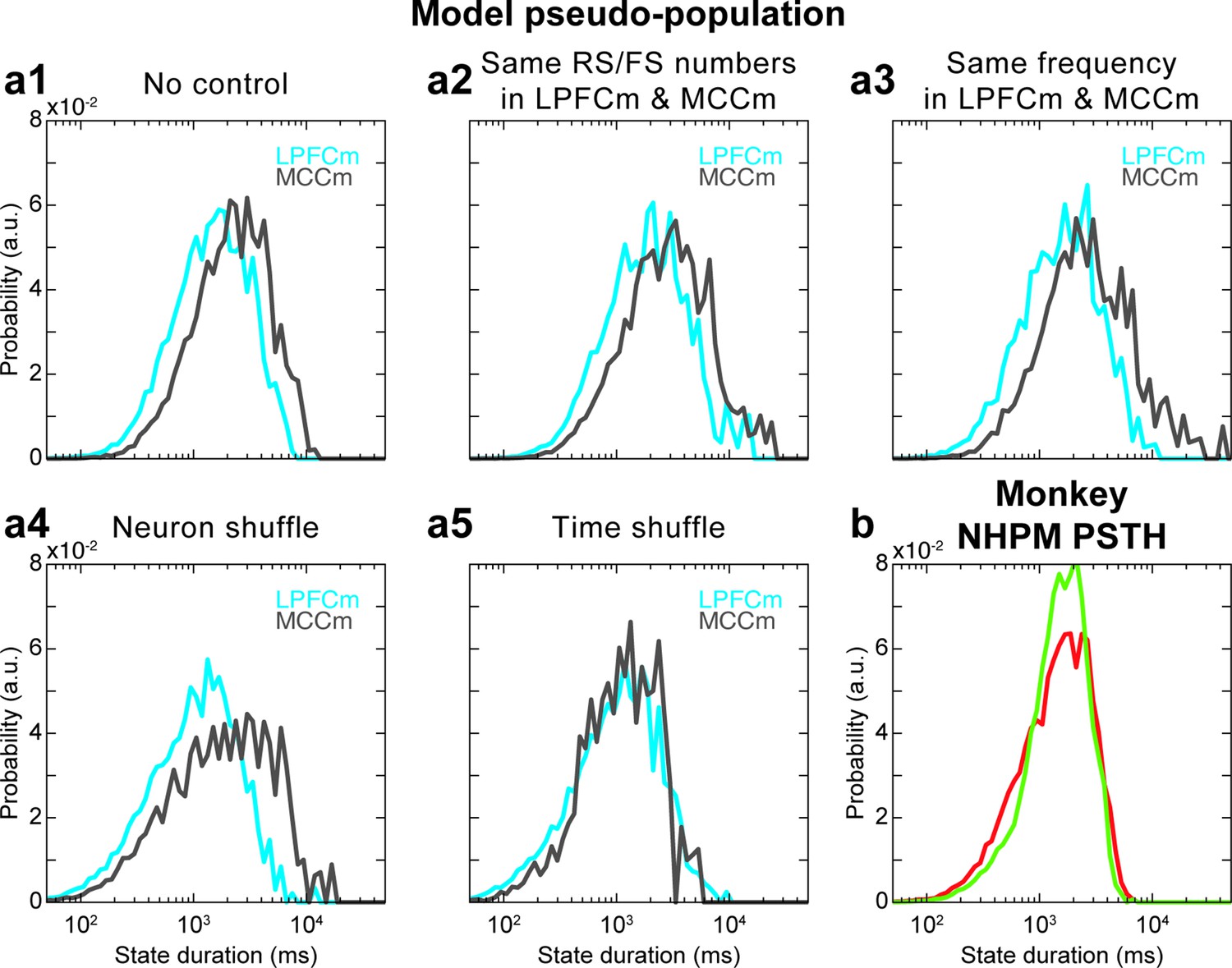
Hidden Markov model (HMM) of model pseudo-population datasets and analysis of the role of task variable coding in HMM analyses.
(a) State duration distributions in the lateral prefrontal cortex (LPFC) (grey) and midcingulate cortex (MCC) (blue) of pseudo-populations built from (a1) model data with a procedure equivalent (see Materials and methods) to monkey data (Figure 7b right), which gives a state duration MCC/LPFC ratio of 1.5 in the absence of control procedure, and for different controls where (a2) group statistics are chosen the same (i.e. those of monkey LPFC group statistics [ratio of 1.52]), (a3) randomly spikes are removed in LPFCm data such that LPFCm and MCCm have precisely the same frequency (ratio of 2.03), (a4) the neural identity is shuffled (the neuron to which each spike is associated is randomly reattributed) (ratio of 1.92) and (a5) the timing of spikes is shuffled in each neuron (ratio of 1.01). Distributions are averaged over 10 independent HMM analyses for each panel. Panels (a1–a4) altogether indicate that state durations are robustly larger in the MCC, compared to the LPFC, even when using pseudo-populations in the model (a1), as quantitatively similar results are obtained even when strong degradations of model data are operated to examine the contribution of possible confounding factors (a2–a4). Panel (a5) indicates that larger state durations in the MCC in model pseudo-populations emerge from the global temporal structure of neural activity in the model. (b) HMM of experimental pseudo-population data where neural spiking activity of each neuron in LPFC and MCC areas is simulated as a non-homogeneous Poisson model (NHPM) whose instantaneous firing rate is given by the post-stimulus time histogram (PSTH) of that neuron within each epoch type between all possible task events (e.g. reward, go signal, etc.). This simulated activity only depends on task-variable coding but does not contain any specific fine-grained activity temporal structure internally generated by frontal areas. There is no difference of state durations between LPFC and MCC, indicating that task variable coding is not responsible for the state duration difference between LPFC and MCC but relies on the precise temporal structure of spiking, independent of task epochs. Thus, accounting for neural states in monkeys with a biophysical model devoid of task structure is not an issue per se.
Figure 7—figure supplement 2
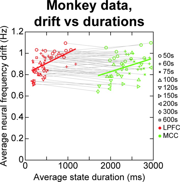
Analysing the correlational relationship between neural frequency drift and Hidden Markov model (HMM) state durations in monkey spike data.
The HMM analysis was repeated on temporal segments of 50 s of the 600 s monkey data (i.e. performed on spike data from 0 to 50 s, 50–100 s, etc. all the way up to 550–600 s). This procedure was repeated for different segment durations (i.e. segments of 50, 60, 75 s, 100, 120, 150, 200, 300, 600 s), to find at which timescale such neural frequency drifts might bias HMM state durations, if at all. In each case, the average neural frequency drift was measured as the absolute difference in neural frequency between the first and second half of the data segment (e.g. 0–25 vs. 25–50 s for first 50 s segment), averaged across all neurons. The average neural frequency drifts are correlated to average HMM state durations within each cortical area when pooling all segment durations (lateral prefrontal cortex [LPFC] [red markers]: rho ~ 0.54, p ~ 9.9*10–5; midcingulate cortex [MCC] [green markers]: rho ~ 0.38, p ~ 8.3*10–3). However, state duration and frequency drift are never correlated when pooling data from both cortical areas, be it within or across temporal subdivisions, indicating that average neural frequency drift does not account for the observed difference in state durations between LPFC and MCC. Four outliers were removed from LPFC and MCC data according to the scaled median absolute deviation of HMM state durations using the standard (rmoutliers MATLAB function).
Figure 7—figure supplement 3
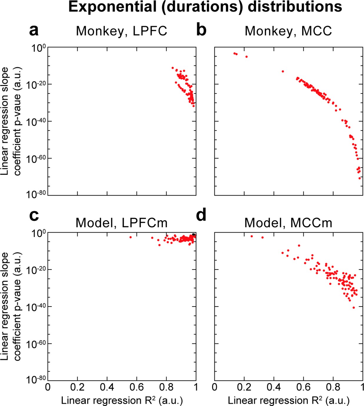
Hidden Markov model (HMM) state durations are distributed exponentially as implied by metastability.
HMM state metastability implies that state durations follow an exponential distribution. Thus, we performed robust linear regressions on the logarithm of the count probability (binned in 50 ms bins) of HMM state durations for each of the 100 HMM analyses, and reported the slope coefficient p-value and R2, for both cortical areas in both monkey and model data. HMM state durations here refer to the durations of each state period, rather than the definition used elsewhere and introduced in the Materials and methods section, being the proportion of time spent in state periods of duration d. We observed overall that R2 scores were above ~0.6, indicating reasonable fits, as well as significantly non-zero slopes (p<0.05, red points; ns: black points) in all monkey HMM analyses, in all MCCm and in the immense majority of PFCm (98/100). Thus, state duration distributions appear exponential, lending credence to the metastable nature of HMM states.
Figure 7—figure supplement 4
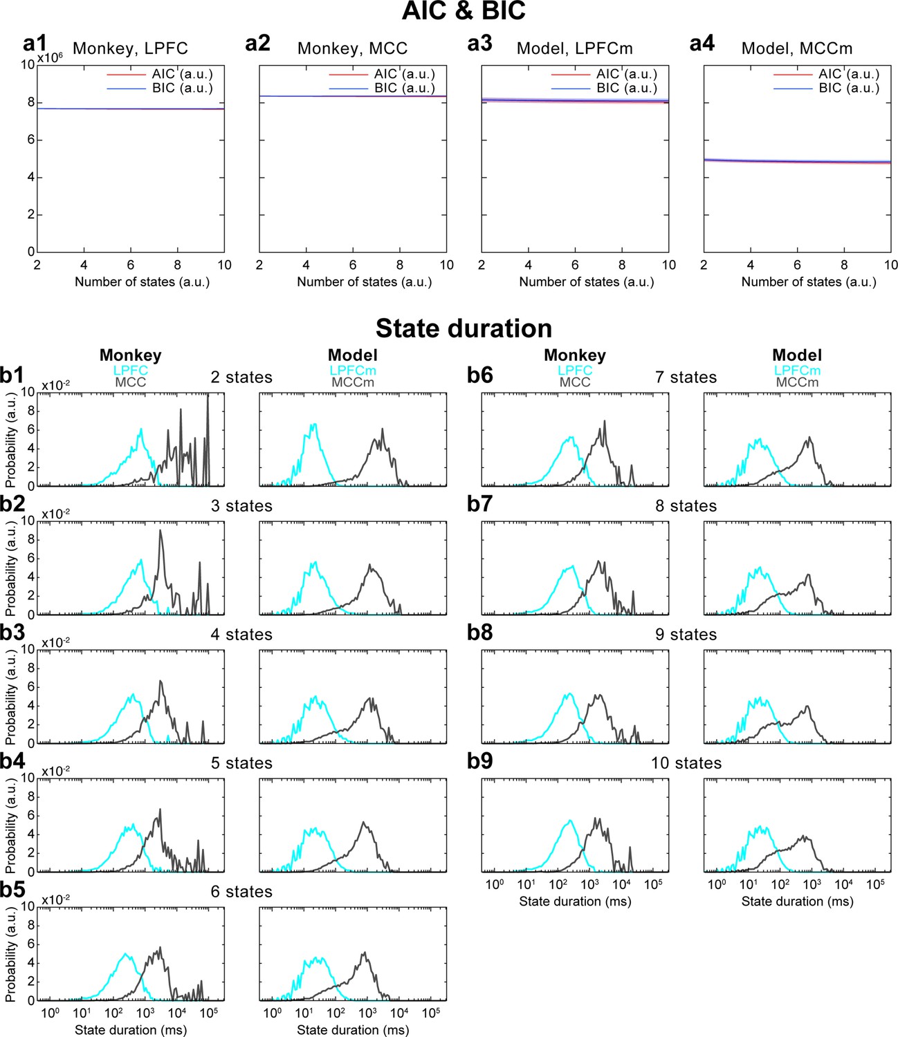
Akaike information criterion (AIC) and Bayesian information criterion (BIC) analysis of the number of Hidden Markov model (HMM) states, and its influence on HMM state durations.
(a) AIC and BIC values for different numbers of states in both cortical areas and in both monkey and model data. AIC and BIC do not substantially change when increasing the number of states. This analysis was repeated five times for each sub-panel. Solid lines are average values, shaded areas are confidence intervals of the mean. (b) When changing the number of states, HMM state duration results did not strongly differ compared to those with four states: while lateral prefrontal cortex (LPFC) and midcingulate cortex (MCC) state durations slightly decreased with more states (since the same time period is divided into a greater number of states), MCC state durations remained one to two orders of magnitude longer than LPFC state durations.
Author response image 1

Author response image 2
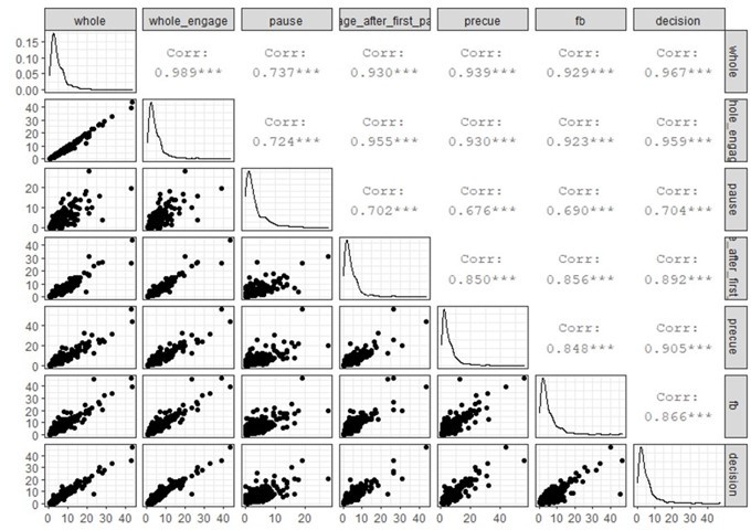
Firing rate correlations computed across different periods.
Author response image 3
Additional files
Download links
A two-part list of links to download the article, or parts of the article, in various formats.
Downloads (link to download the article as PDF)
Open citations (links to open the citations from this article in various online reference manager services)
Cite this article (links to download the citations from this article in formats compatible with various reference manager tools)
Inhibitory control of frontal metastability sets the temporal signature of cognition
eLife 11:e63795.
https://doi.org/10.7554/eLife.63795


