Automated annotation of birdsong with a neural network that segments spectrograms
- Department of Brain Sciences, Weizmann Institute of Science, Israel
- Biology department, Emory University, United States
- Biology department, Boston University, United States
- Phil and Penny Knight Campus for Accelerating Scientific Impact, University of Oregon, United States
Figures
Figure 1 with 2 supplements

Manual annotation of birdsong.
(A) Schematic of the standard two-step process for annotating song by hand (e.g. with a GUI application). Top axes show a spectrogram generated from a brief clip of Bengalese finch song, with different syllable types. Middle and bottom axes show the steps of annotation: first, segments are extracted from song by setting a threshold (’thr.’, dashed horizontal line, bottom axes) on the amplitude and then finding continuous periods above that threshold (colored regions of amplitude trace, bottom axes). This produces segments (colored bars, middle axes) that an expert human annotator manually labels (characters above colored bars), assigning each segment to one of the syllable classes that the annotator defines for each individual bird. (B) Examples showing how the standard approach of segmenting with a fixed amplitude threshold does not work well for canary song. Above threshold amplitudes are plotted as thicker colored lines. For a fixed threshold (dotted line, bottom axes), syllables of type ’b’ are correctly segmented, but syllables of type 'a' are incorrectly segmented into two components, and syllables of type 'c' are not segmented.
Figure 1—figure supplement 1
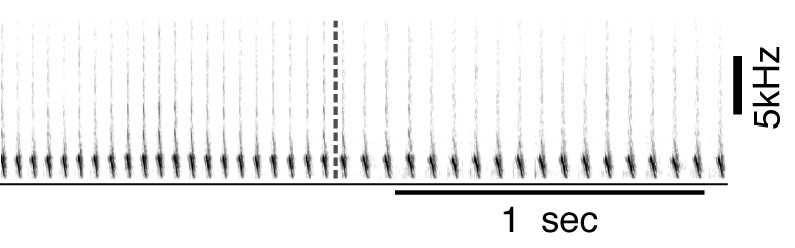
Example of two consecutive canary phrases that differ mostly in inter-syllable gaps.
In this case, annotation methods that first segment syllables and then use acoustic parameters to classify them will introduce errors. By simultaneously learning acoustic and sequence properties, TweetyNet overcomes this weakness.
Figure 1—figure supplement 2
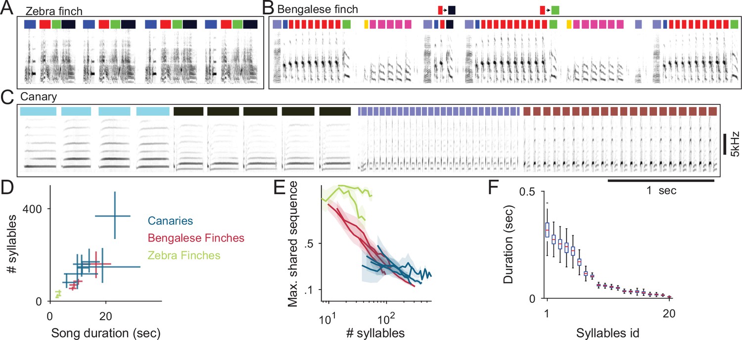
Comparison of descriptive statistics of birdsong syllables across species.
(A) The zebra finch repeating motif allows annotation by matching its template spectrogram without segmenting different syllables (colored bars). (B) Bengalese finch songs segmented to syllables shows variable transitions and changing numbers of syllable repeats. (C) A third of one domestic canary song of median duration segmented to syllables reveals repetitions (phrase) structure. (D) The median, 0.25 and 0.75 quantiles of song durations (x-axis) and number of syllables per song (y-axis) for two canary strains, Bengalese finches and Zebra finches (color coded) (E) Variable songs are not suited for template matching. Songs contain repeating sequences of syllables but because of sequence variability songs with more syllables (x-axis) share smaller sequence fractions (y-axis) (F) Distributions of syllable duration for one domestic canary. The bird had 20 different syllable types (x-axis, ordered by mean syllable duration). Box plot shows median, 0.25 and 0.75 quantiles of syllable durations. Whiskers show the entire range.
Figure 2
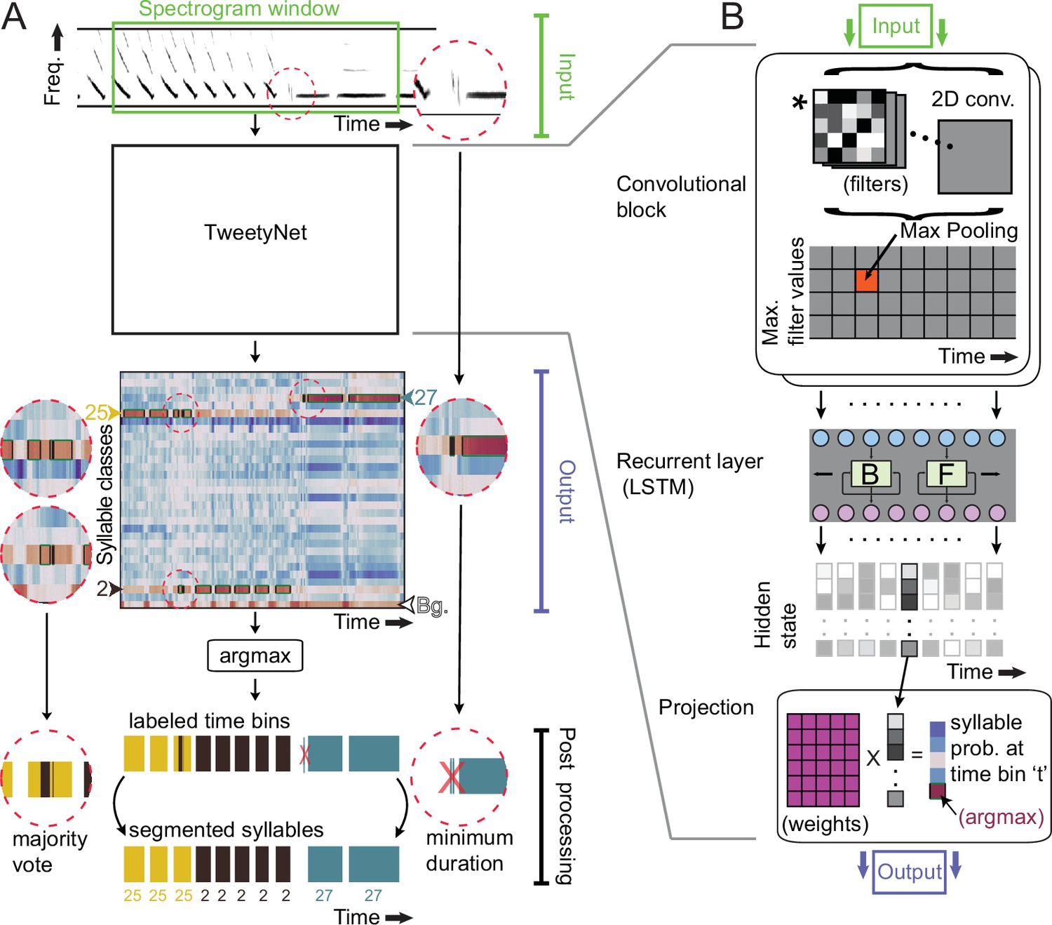
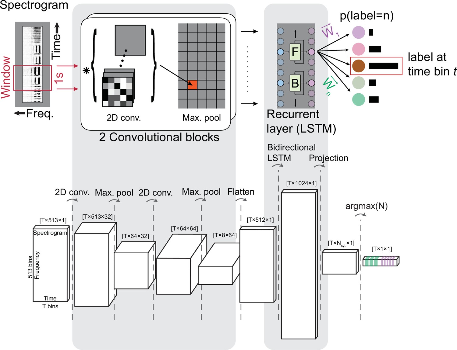
TweetyNet operation and architecture.
(A) TweetyNet takes as input a window from a spectrogram, and produces as output an estimate of the probability that each time bin in the spectrogram window belongs to a class from the set of predefined syllable classes . This output is processed to generate the labeled segments that annotations are composed of: (1) We apply the argmax operation to assign each time bin the class with the highest probability. (2) We use the ‘background’ class we add during training (indicated as ‘Bg.’) to find continuous segments of syllable class labels. (3) We post-process these segments, first discarding any segment shorter than a minimum duration (dashed circle on right side) and then taking a majority vote to assign each segment a single label (dashed circles on left side). (B) TweetyNet maps inputs to outputs through a series of operations: (1) The convolutional blocks produce a set of feature maps by convolving (asterisk) their input and a set of learned filters (greyscale boxes). A max-pooling operation downsamples the feature maps in the frequency dimension. (2) The recurrent layer, designed to capture temporal dependencies, is made up of Long Short Term Memory (LSTM) units. We use a bidrectional LSTM that operates on the input sequence in both the forward (F) and backward (B) directions to produce a hidden state for each time step, modulated by learned weights in the LSTM units. (3) The hidden states are projected onto the different syllable classes by a final linear transformation, resulting in a vector of class probabilities for each time bin . For further details, please see section ‘Neural network architecture’ in Materials and methods.
Figure 3
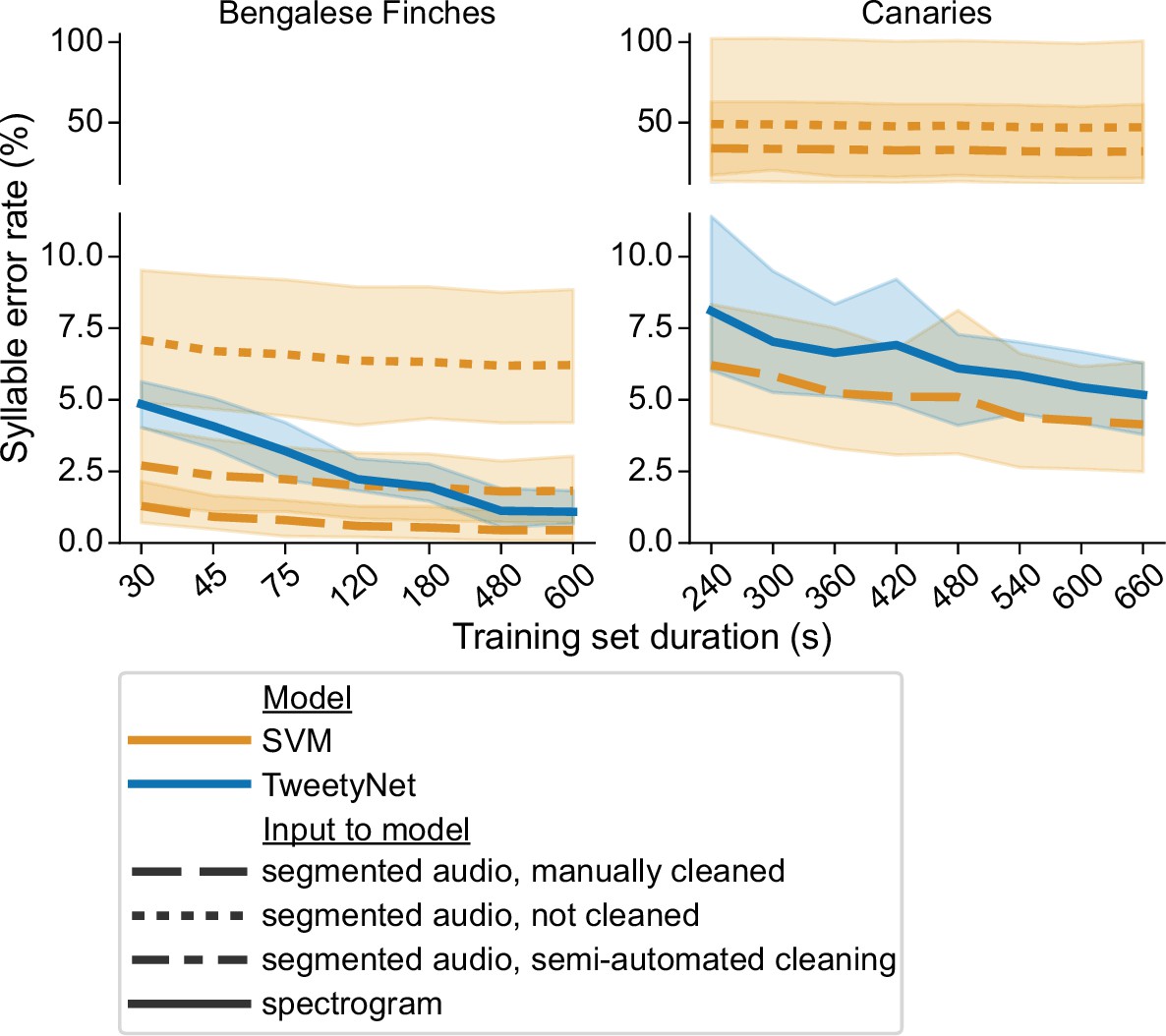
Comparison of TweetyNet with a support vector machine (SVM) model.
Plots show syllable error rate (y axis) as a function of training set size (x axis, size of training set in seconds). Syllable error rate is an edit distance computed on sequences of text labels. Here it is measured on a fixed, held-out test set (never seen by the model during training). Hues correspond to model type: TweetyNet neural network (blue) or SVM (orange). Shaded areas around lines indicate the standard deviation across song of individual birds, and across model training replicates (each trained with different subsets of data randomly drawn from a total training set, n = 4 Bengalese finches, 10 replicates per bird;n = 3 canaries, 7 replicates per bird). Line style indicates input to model: spectrogram (solid line), or segmented audio, processed in three different ways, either manually cleaned by human annotators (dashed), not cleaned at all (dotted), or cleaned with a semi-automatic approach (dot-dash).
-
Figure 3—source data 1
Data used to generate line plots.
- https://cdn.elifesciences.org/articles/63853/elife-63853-fig3-data1-v2.csv
Figure 4

Performance of TweetyNet across songs of 8 Bengalese finches and three canaries.
Plots show frame error (y axis, top row) and syllable error rate (y axis, bottom row) as a function of training set size (x axis, in seconds). Frame error is simple accuracy of labels the network predicted for each time bin in spectrograms, while syllable error rate is an edit distance computed on sequences of labels for the segments that we recover from the vectors of labeled time bins (as described in main text). Thick line is mean across all individuals, thinner lines with different styles correspond to individual birds (each having a unique song). Shaded areas around lines for each bird indicate standard deviation of metric plotted across multiple training replicates, each using a different randomly-drawn subset of the training data. Metrics are computed on a fixed test set held constant across training replicates. Here hue indicates species (as in Figure 5A below): Bengalese finches (magenta, left column) and canaries (dark gray, right column).
-
Figure 4—source data 1
Data used to generate plots for Bengalese finches.
- https://cdn.elifesciences.org/articles/63853/elife-63853-fig4-data1-v2.csv
-
Figure 4—source data 2
Data used to generate plots for canaries.
- https://cdn.elifesciences.org/articles/63853/elife-63853-fig4-data2-v2.csv
Figure 5 with 4 supplements
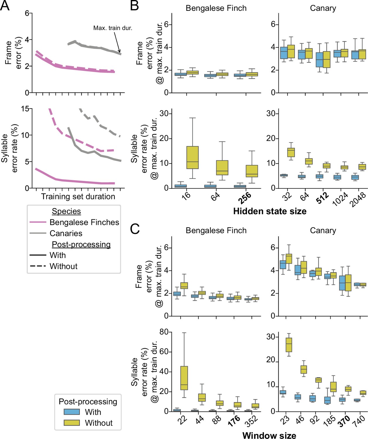
The effect of post-processing and hyperparameters on TweetyNet performance.
(A) Mean frame error (top row) and mean syllable error rate, across all birds and training replicates, as a function of training set duration. Hue indicates species (Bengalese finches, magenta; canaries, dark gray). Line style indicates whether the metric was computed with (solid lines) or without (dashed lines) post-processing of the vectors of labeled time bins that TweetyNet produces as output. (Note solid lines are same data as Figure 4). (B, C). Performance for a range of values for two key hyperparameters: the size of windows from spectrograms shown to the network (B) and the size of the hidden state in the recurrent layer (C). Box-and-whisker plots show metrics computed at the maximum training set duration we used for the curves in A (‘Max. train dur.’, black arrow in A). We chose the maximum training set durations because at those metrics were closest to the asymptotic minimum approached by the learning curves. Top row of axes in both B and C shows frame error, and bottom row of axes shows syllable error rate. Blue boxes are metrics computed with post-processing transforms applied, orange boxes are error rates without those transforms. Ticks labels in boldface on axes in B and C represent the hyperparameters we used for results shown in A, and Figures 3 and 4.
-
Figure 5—source data 1
Data used to generate line plots in Figure 5A, B, Figure 5—figure supplement 3.
- https://cdn.elifesciences.org/articles/63853/elife-63853-fig5-data1-v2.csv
-
Figure 5—source data 2
Data used to generate box plots in Figure 5B, C, Figure 5—figure supplement 3.
- https://cdn.elifesciences.org/articles/63853/elife-63853-fig5-data2-v2.csv
Figure 5—figure supplement 1
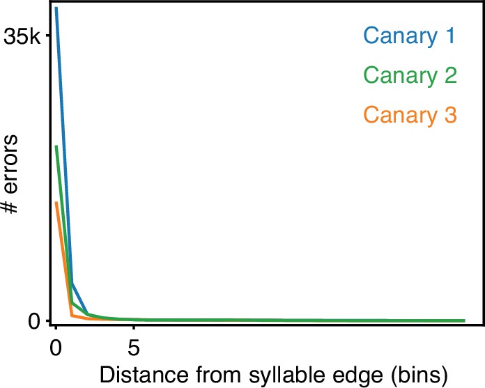
Most frame errors of trained TweetyNet models are disagreement on syllable boundaries of 0–2 time bins.
Potential syllable boundary disagreements are time bins in which the ground truth test set or the trained TweetyNet model disagree and just one of them assigns the ’background’ label. The histograms show the distances of those time bins from the nearest syllable boundary in test sets 5000 second long.
Figure 5—figure supplement 2
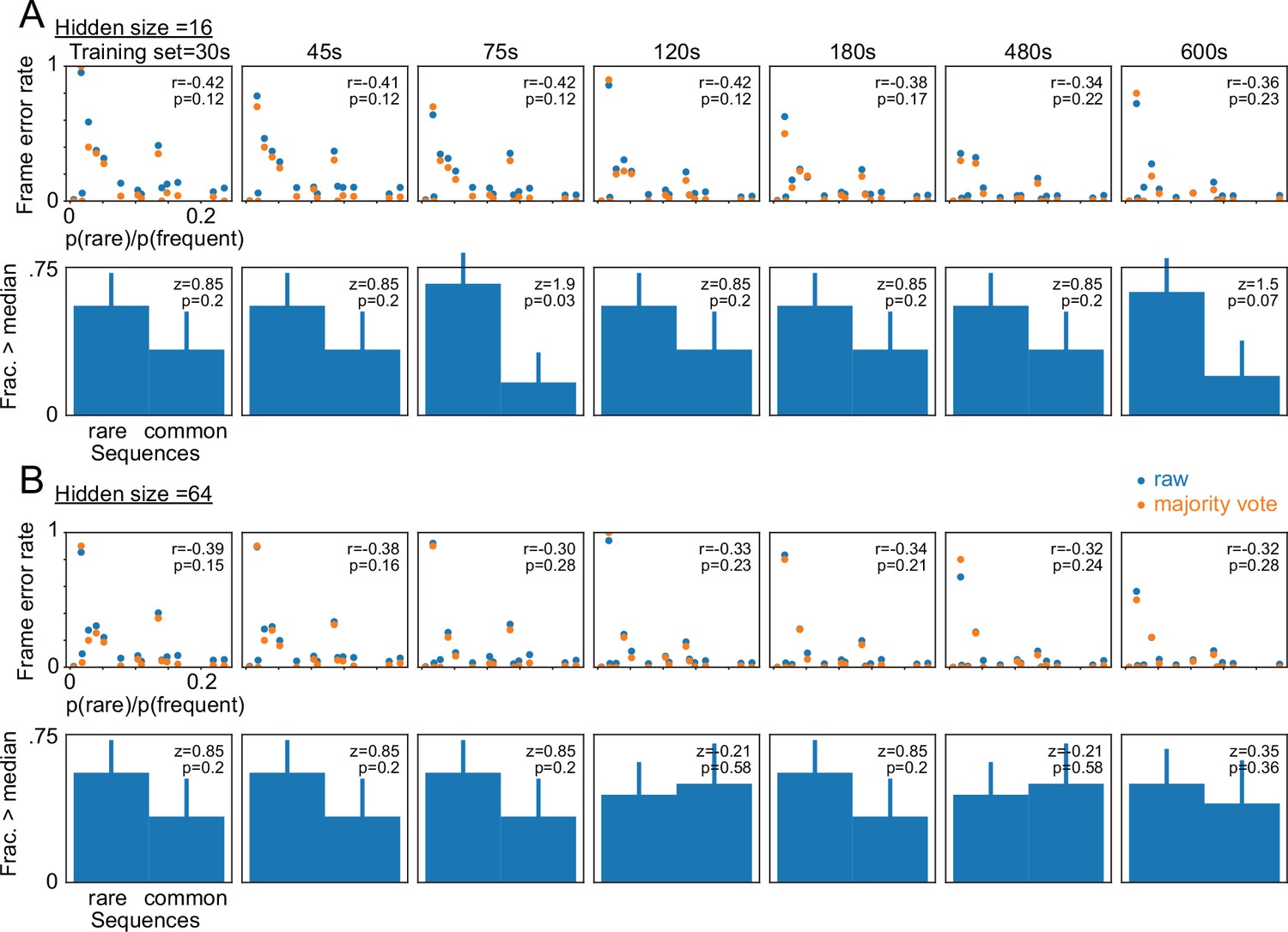
frame errors in rarely-occurring Bengalese finch sequences.
Each dot represents a syllable sequence a-b-y. The x-axis shows the ratio between the frequency of a-b-y and the frequency of the most common sequence a-b-x (p(rare) and p(frequent) respectively). The y-axis shows the frame error measured in the segments y occurring in the context a-b-y. (A) TweetyNet models with very small hidden state sizes will have large error rates in some, but not all, of the rarely occurring events. This is seen in the negative Pearson correlation (top panel, r values) between the error rate (y-axis) and the relative rarity of the sequence (x-axis) and in larger fractions of above-median error rates in the more rare events compared to the more common among the data in the top panel (Bars, bottom panel. Error bars showing S.E.). These effects are almost never significant (Pearson r,p in the top panels and the binomial z-test and p values in the bottom panels) and decrease if applying the majority vote transform (orange dots) or when training the networks with more data (left to right panels showing training sets 30–600 s long). Note these results are from networks trained with a hidden state size of 16. For main results in Figures 5A and 6 we used a size of 256. (B) Repeats A but with hidden state size of 64, and showing an even smaller effect.
Figure 5—figure supplement 3
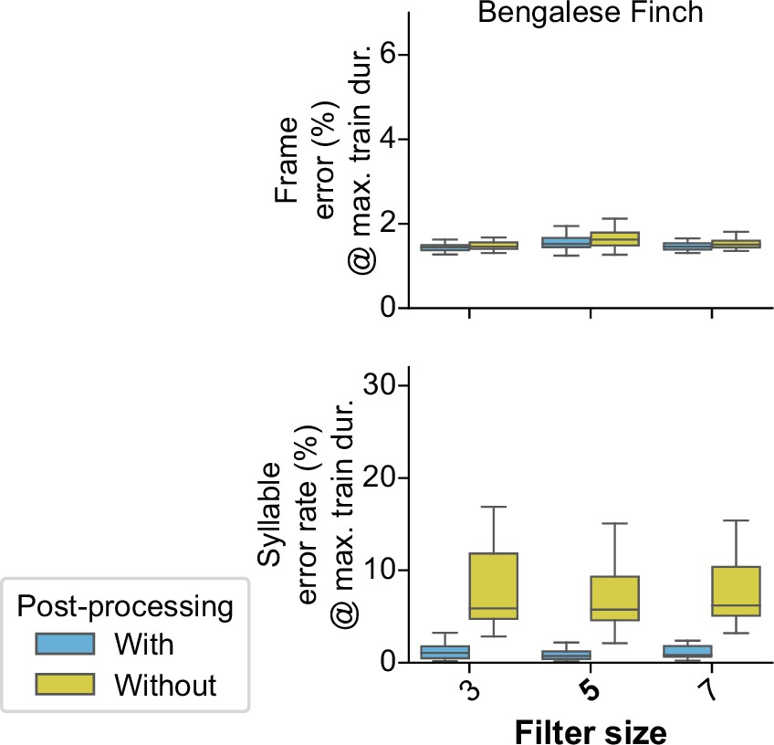
Filter size experiments.
Figure 5—figure supplement 4
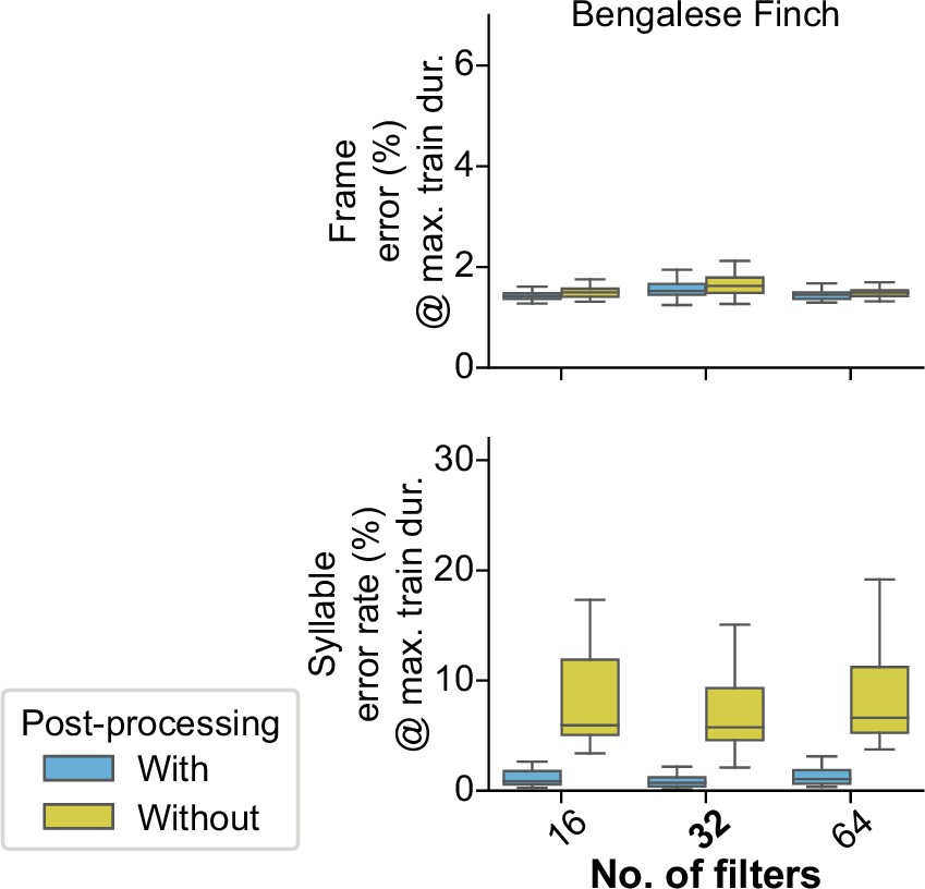
Filter number experiments.
Figure 6
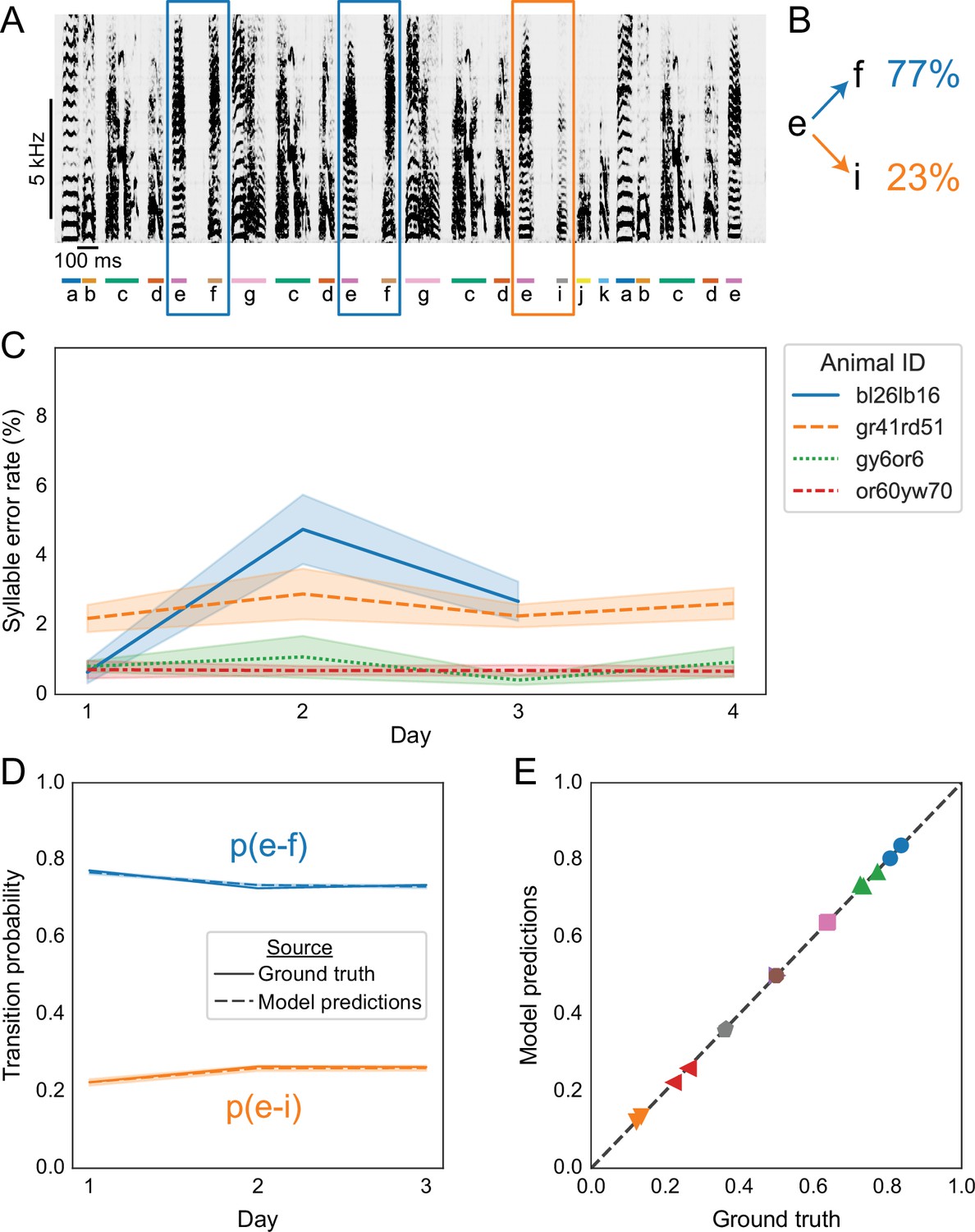
Replicating results on branch points in Bengalese finch song with annotations predicted by TweetyNet.
(A) Representative example of a Bengalese finch song with a branch point: the syllable labeled ’e’ can transition to either ’f’, as highlighted with blue rectangles, or to ’i’, as highlighted with an orange rectangle. (B) Transition probabilities for this branch point, computed from one day of song. (C) Syllable error rates per day for each bird from Nicholson et al., 2017. Solid line is mean and shaded area is standard deviation across 10 training replicates. Line color and style indicate individual animals. TweetyNet models were trained on 10 min of manually annotated song, a random subset drawn from data for day 1. Then syllable error rates were computed for the remaining songs from day 1, and for all songs from all other days. (D) Transition probabilities across days for the branch point in A and B, computed from the ground truth annotations (solid lines) and the annotations predicted by TweetyNet (dashed lines). Shaded area around dashed lines is standard deviation of the estimated probabilities, across the 10 training replicates. (E) Group analysis of transition. x axis is probability computed from the ground truth annotations, and the y axis is probability estimated from the predicted annotations. Dashed line is ‘x = y’, for reference. Each (color, marker shape) combination represents one branch point from one bird.
-
Figure 6—source data 1
Data used to generate line plot in Figure 6C.
- https://cdn.elifesciences.org/articles/63853/elife-63853-fig6-data1-v2.csv
-
Figure 6—source data 2
Data used to generate line plot in Figure 6D.
- https://cdn.elifesciences.org/articles/63853/elife-63853-fig6-data2-v2.csv
-
Figure 6—source data 3
Data used to generate scatter plot in Figure 6E.
- https://cdn.elifesciences.org/articles/63853/elife-63853-fig6-data3-v2.zip
Figure 7 with 2 supplements
Replicating and extending results about canary syntax dependencies with annotations predicted by TweetyNet.
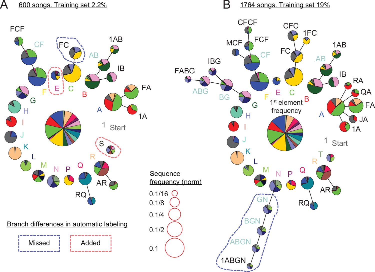
(A) Long-range order found in 600 domestic canary songs annotated with human proof reader (methods, similar dataset size to Markowitz et al., 2013). Letters and colors indicate phrase types. Each branch terminating in a given phrase type indicates the extent to which song history impacts transition probabilities following that phrase. Each node corresponds to a phrase sequence, annotated in its title, and shows a pie chart representing the outgoing transition probabilities from that sequence (e.g. the pie ’1A’ shows the probabilities of phrases ’B’, ’C’, and ’F’ which follow the phrase sequence ’1→ A’). The nodes are scaled according to their frequency (legend). Nodes that can be grouped together (chunked as a sequence) without significantly reducing the power of the model are labeled with blue text. These models are built by iterative addition of nodes up the branch to represent longer Markov chains, or a transition's dependence on longer sequences of song history. A TweetyNet model was trained using 2.2% of 1,764 songs (9.5% of the data in A). The PST created from the model’s predicted annotation of the entire dataset is very similar to A (see full comparison in Figure 7—figure supplement 1). Here, branch differences between the hand labeled and model labeld song are marked by red and blue dashed lines for added and missed branches. (B) PST created using all 1,764 hand labeled songs. An almost identical PST was created without a human proof reader from a TweetyNet model trained on 19% of the data (see full comparison in Figure 7—figure supplement 2).
Figure 7—figure supplement 1
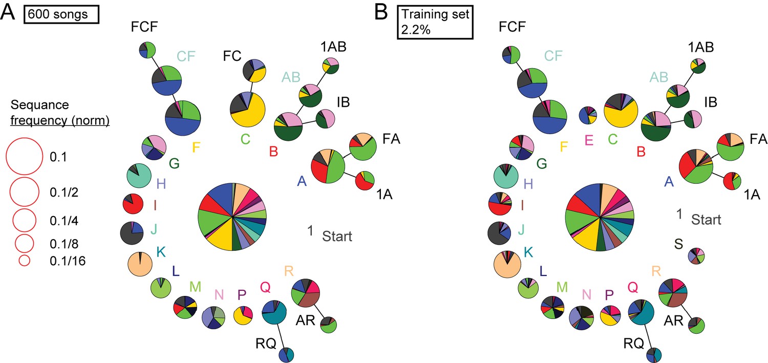
Detailed comparison of syntax structure in 600 hand labeled or TweetyNet-labeled canary songs.
We plot the full probabilistic suffix trees created from 600 hand labeled canary songs (A) and from the prediction of a TweetyNet model trained on 2.2% of this bird’s song (B).
Figure 7—figure supplement 2
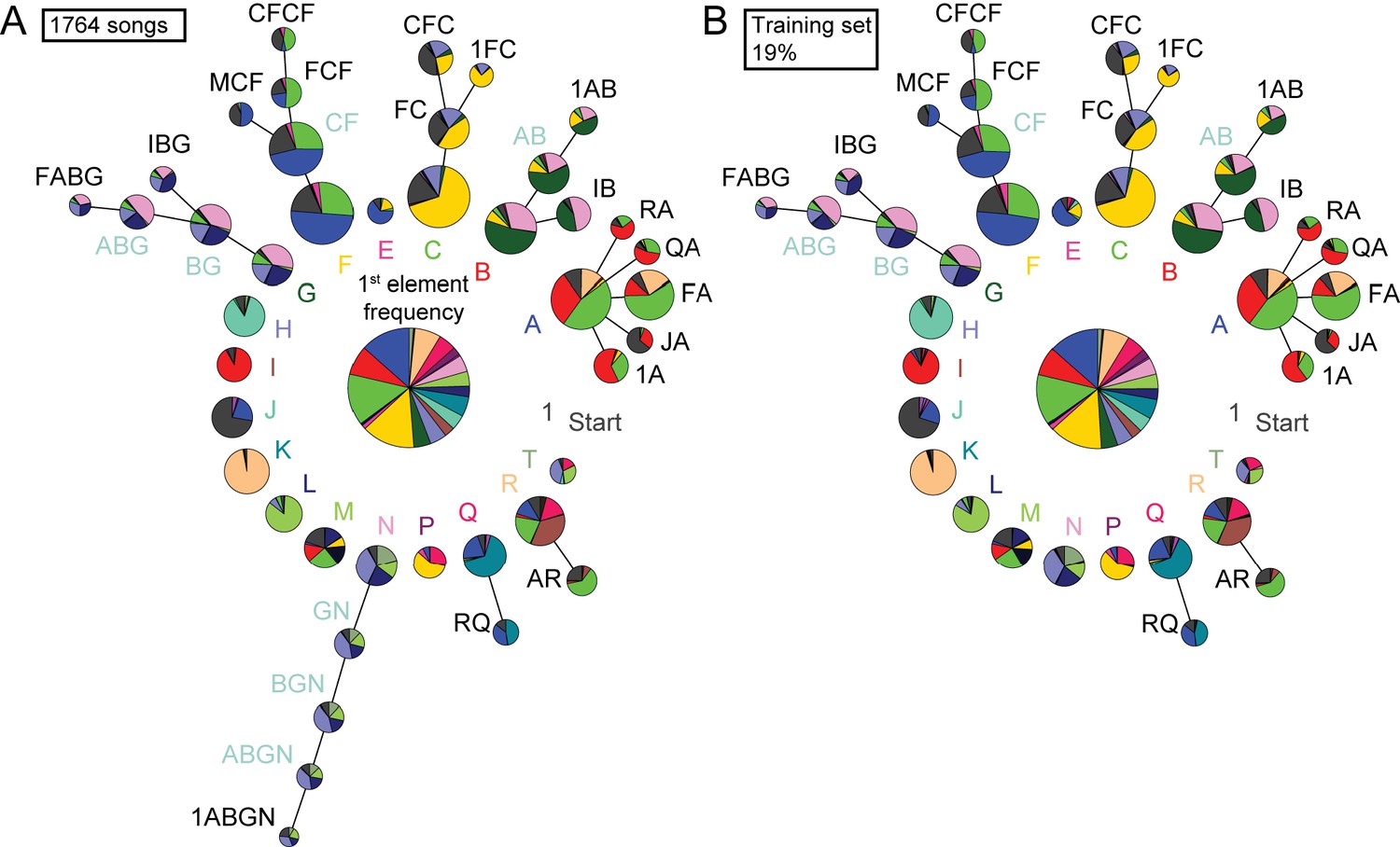
Detailed comparison of syntax structure in 1764 hand labeled or TweetyNet-labeled canary songs.
Supporting Figure 7B. We plot the full probabilistic suffix trees created from 1,764 hand labeled canary songs (A) and from the prediction of a TweetyNet model trained on 19% of this bird’s song (B). The fluctuation in transition probabilities accumulates in long sequences and, in this example, increases the minimal sequence probability included in the PST. This increase prevented the inclusion of the ’N’ branch in the model built on TweetyNet’s prediction.
Figure 8
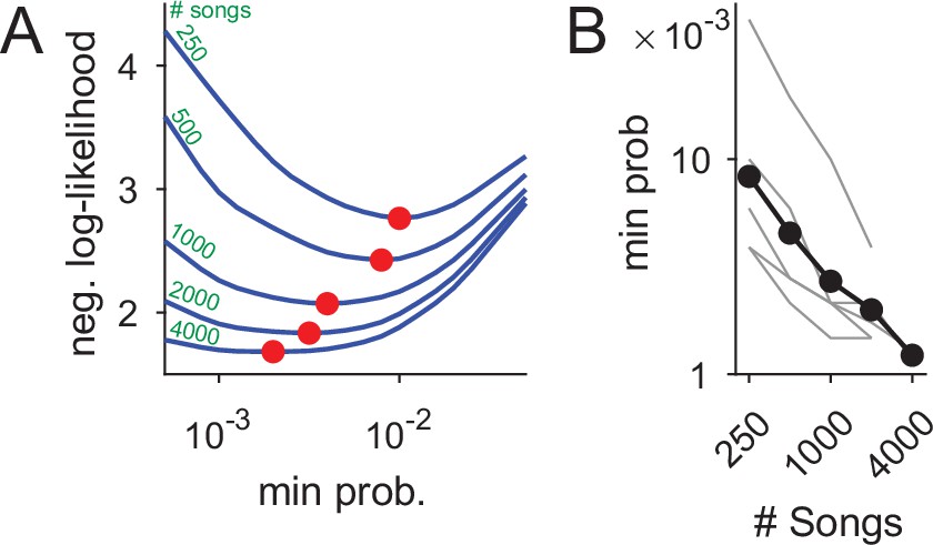
Using datasets more than five times larger than previously explored increases statistical power and the precision of syntax models.
(A) Ten-fold cross validation is used in selection of the minimal node probability for the PSTs (x-axis). Lines show the mean negative log-likelihood of test set data estimated by PSTs in 10 repetitions (methods). Curves are calculated for datasets that are sub sampled from about 5000 songs. Red dots show minimal values - the optimum for building the PSTs. (B) The decrease in optimal minimal node probability (y-axis, red dots in panel A) for increasing dataset sizes (x-axis) is plotted in gray lines for six birds. The average across animals is shown in black dots and line.
-
Figure 8—source data 1
Data used to generate lines in Figure 8A.
- https://cdn.elifesciences.org/articles/63853/elife-63853-fig8-data1-v2.csv
-
Figure 8—source data 2
Data used to generate dots in Figure 8A.
- https://cdn.elifesciences.org/articles/63853/elife-63853-fig8-data2-v2.csv
-
Figure 8—source data 3
Data used to generate lines in Figure 8B.
- https://cdn.elifesciences.org/articles/63853/elife-63853-fig8-data3-v2.csv
Figure 9

Rare variants of canary song introduce segmentation and annotation errors.
(A-E) Spectrograms on top of the time-aligned likelihood (gray scale) assigned by a well-trained TweetyNet model to each of the labels (y-axis, 30 syllable types and the tag ’Bg.’ for the background segments). Green and red vertical lines and numbers on top of the spectrograms mark the onset, offset, and labels predicted by the model. (A,B) Canary phrase transitions can contain a vocalization resembling the two flanking syllables fused together. A TweetyNet model trained to split this vocalization performed very well (A) but failed in a rare variant (B). The network output highlights a general property: TweetyNet assigned high likelihood to the same flanking syllable types and not to irrelevant syllables. (C) Syllables produced soft, weak, and acoustically imprecise at the onset of some canary phrases are mostly captured very well by TweetyNet but, on rare occasions, can be missed. In this example the model assigned high likelihood to the correct label but higher to the background. (D) Some human annotators, called 'splitters', define more syllable classes. Others, the 'lumpers', group acoustically-diverse vocalizations under the same label. TweetyNet models trained on acoustically-close classes assign high likelihood to both labels and, on rare occasions, flip between them. This example demonstrates that TweetyNet does not use the a-priori knowledge of syllable repeats hierarchically-forming canary phrases. (E) Canaries can simultaneously produce two notes from their two bronchi. This occurs in phrase transitions and the spectrogram of the resulting vocalization resembles an overlay of flanking syllables. While the network output shows high likelihood for both syllables the algorithm is forced to choose just one.
Figure 10
TweetyNet architecture and tensor shapes resulting from each operation in the network.
Additional files
Download links
A two-part list of links to download the article, or parts of the article, in various formats.
Downloads (link to download the article as PDF)
Open citations (links to open the citations from this article in various online reference manager services)
Cite this article (links to download the citations from this article in formats compatible with various reference manager tools)
Automated annotation of birdsong with a neural network that segments spectrograms
eLife 11:e63853.
https://doi.org/10.7554/eLife.63853


