Relative demographic susceptibility does not explain the extinction chronology of Sahul’s megafauna
- Global Ecology Partuyarta Ngadluku Wardli Kuu, College of Science and Engineering, Flinders University, Australia
- ARC Centre of Excellence for Australian Biodiversity and Heritage, Australia
- Dynamics of Eco-Evolutionary Pattern, University of Tasmania, Australia
- College of Science and Engineering, Flinders University, Australia
- Faculty of Biological and Environmental Sciences, University of Helsinki, Finland
Figures
Figure 1
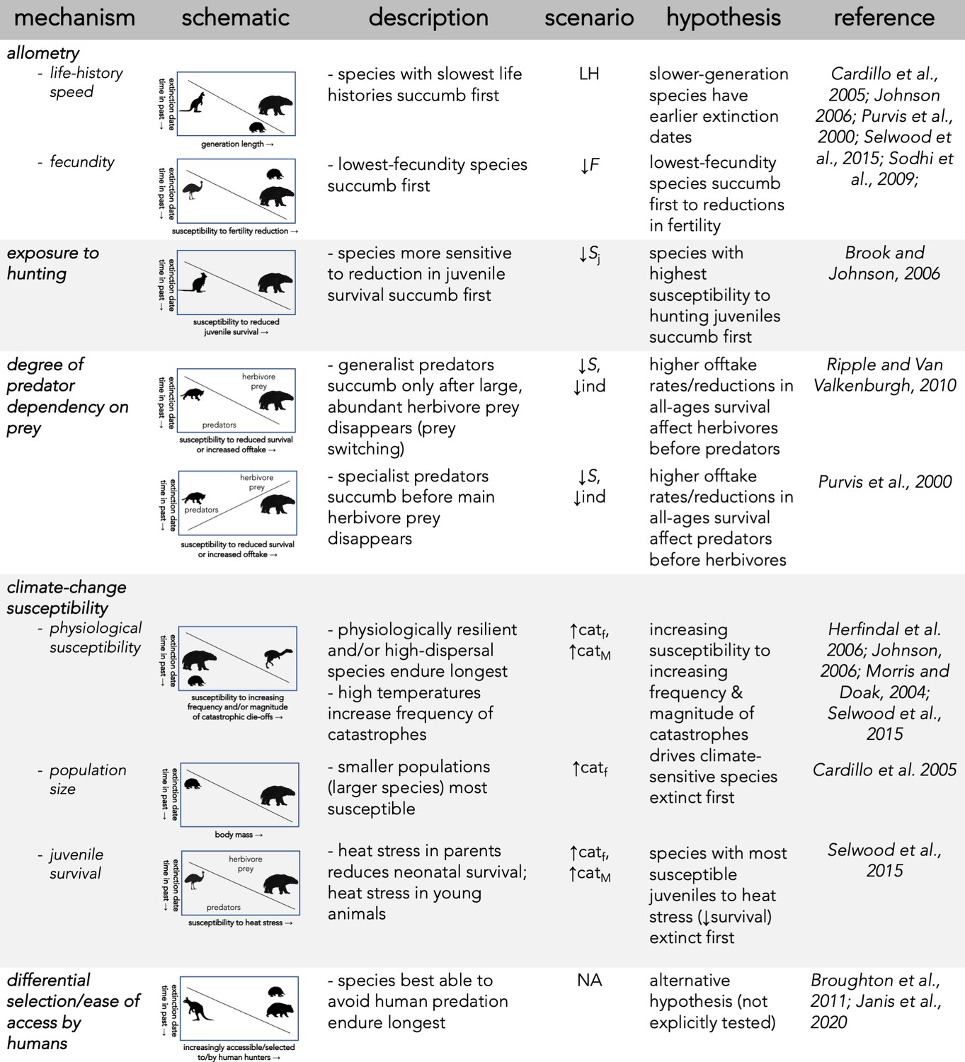
Description of five dominant mechanisms by which megafauna could have been driven to extinction and the associated seven perturbation scenarios examined.
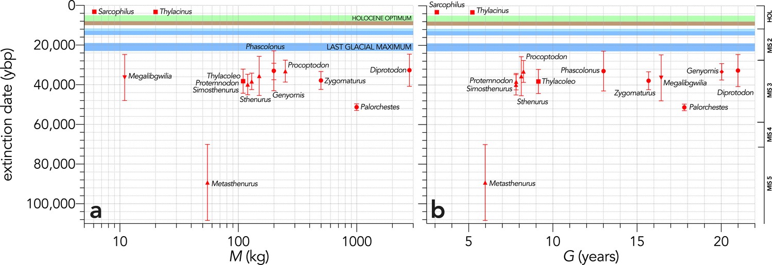
Figure 2
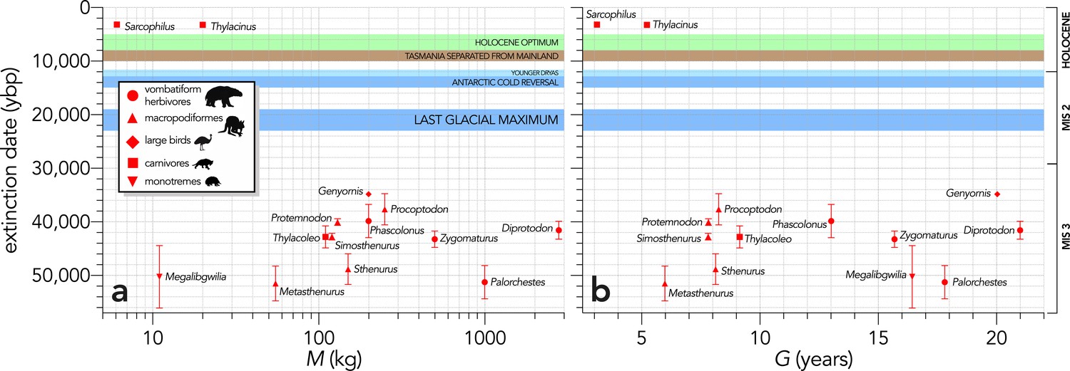
Relationship between estimated date of species extinction (across the entire continent) and (a) body mass (M, kg) or (b) generation length (G, years) (Scenario LH).
Extinction-timing windows are estimated based on the agreement among six different models that correct for the Signor-Lipps effect (described in Materials and methods) in chronologies of quality-rated (Rodríguez-Rey et al., 2015) fossil dates for the studied taxa described in Peters et al., 2019. Here, we have depicted Sarcophilus as ‘extant’, even though it went extinct on the mainland >3000 years ago. Also shown are the approximate major climate periods and transitions: Marine Isotope Stage 3 (MIS 3), MIS 2 (including the Last Glacial Maximum, Antarctic Cold Reversal, and Younger Dryas), and the Holocene (including the period of sea level flooding when Tasmania separated from the mainland, and the relatively warm, wet, and climatically stable Holocene optimum).
Figure 3
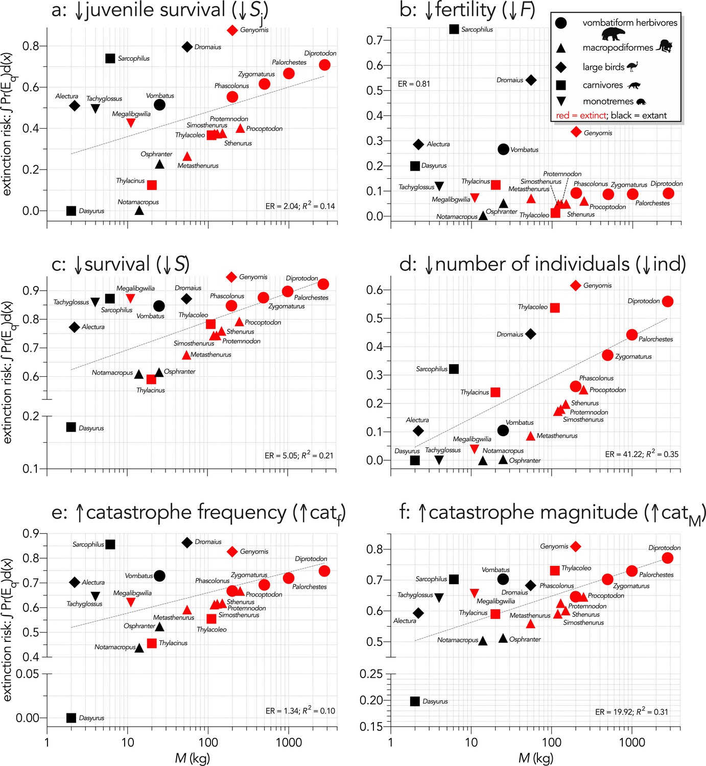
Area under the quasi-extinction curve (from Appendix 6—figure 1) — extinction risk: ∫Pr(Eq)d(x) — as a function of body mass (M, kg) for (a) (Scenario ↓Sj) decreasing juvenile survival, (b) (Scenario ↓F) decreasing fertility, (c) (Scenario ↓S) decreasing survival across all age classes, (d) (Scenario ↓ind) increasing number of individuals removed year−1, (e) (Scenario ↑catf) increasing frequency of catastrophic die-offs per generation, and f: (Scenario ↑catM) increasing magnitude of catastrophic die-offs.
Shown are the information-theoretic evidence ratios (ER) and variation explained (R2) for the lines of best fit (grey dashed) in each scenario. Here, we have depicted Sarcophilus as ‘extant’, even though it went extinct on the mainland >3000 years ago.
Figure 4
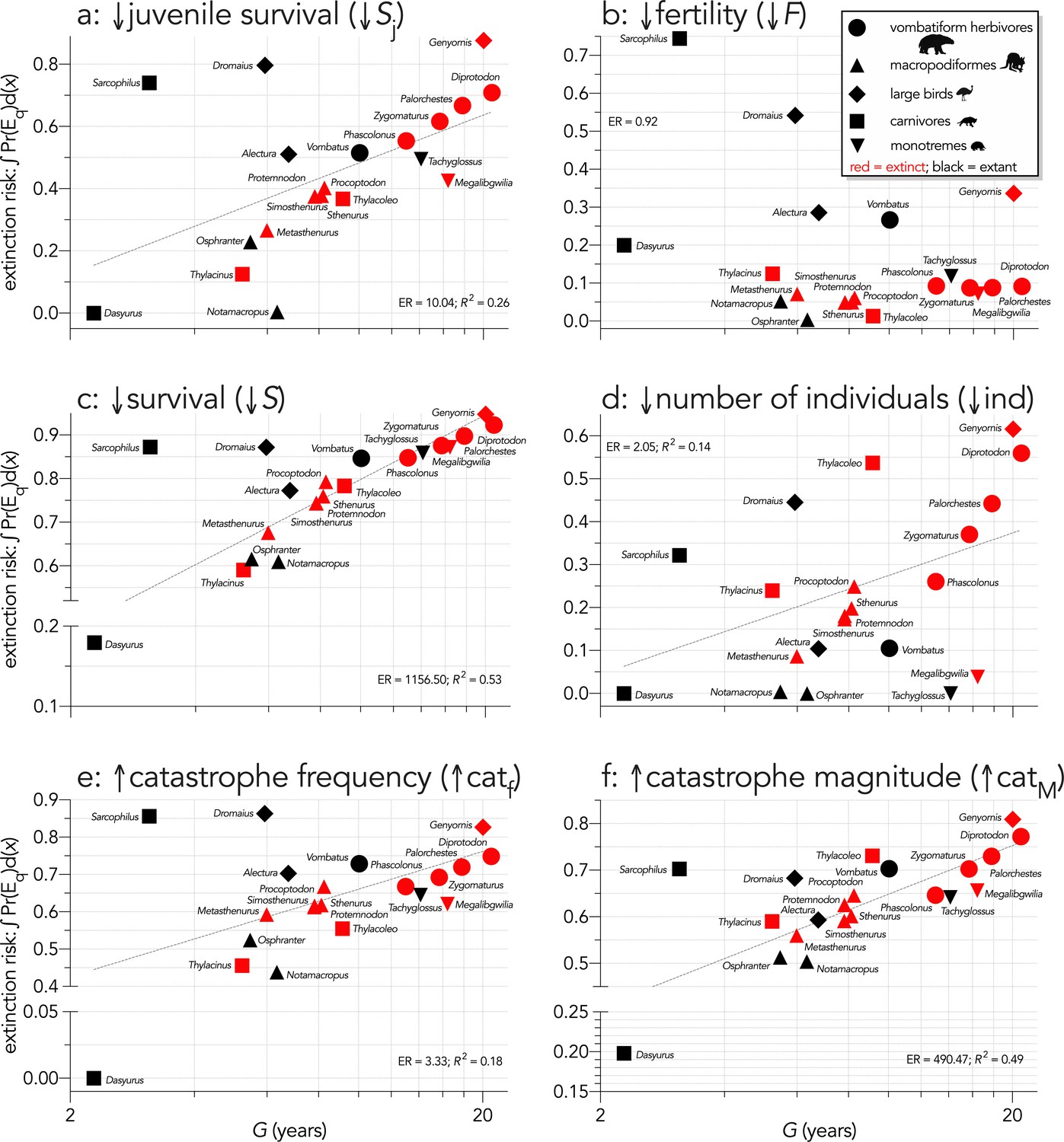
Area under the quasi-extinction curve (from Appendix 6—figure 1) — extinction risk: ∫Pr(Eq)d(x) — as a function of generation length (G, years) for (a) (Scenario ↓Sj) decreasing juvenile survival, (b) (Scenario ↓F) decreasing fertility, (c) (Scenario ↓S) decreasing survival across all age classes, (d) (Scenario ↓ind) increasing number of individuals removed year−1, (e) (Scenario ↑catf) increasing frequency of catastrophic die-offs per generation, and f: (Scenario ↑catM) increasing magnitude of catastrophic die-offs.
Shown are the information-theoretic evidence ratios (ER) and variation explained (R2) for the lines of best fit (grey dashed) in each scenario. Here, we have depicted Sarcophilus as ‘extant’, even though it went extinct on the mainland >3000 years ago.
Figure 5

Inset: Increasing extinction risk for birds — quasi-extinction probability: Pr(Eq) — as a function of increasing the mean number of eggs harvested per female per year (Scenario ↓Fe).
The main graph shows the area under the quasi-extinction curve — extinction risk: ∫Pr(Eq)d(x) — as a function body mass (M, kg).
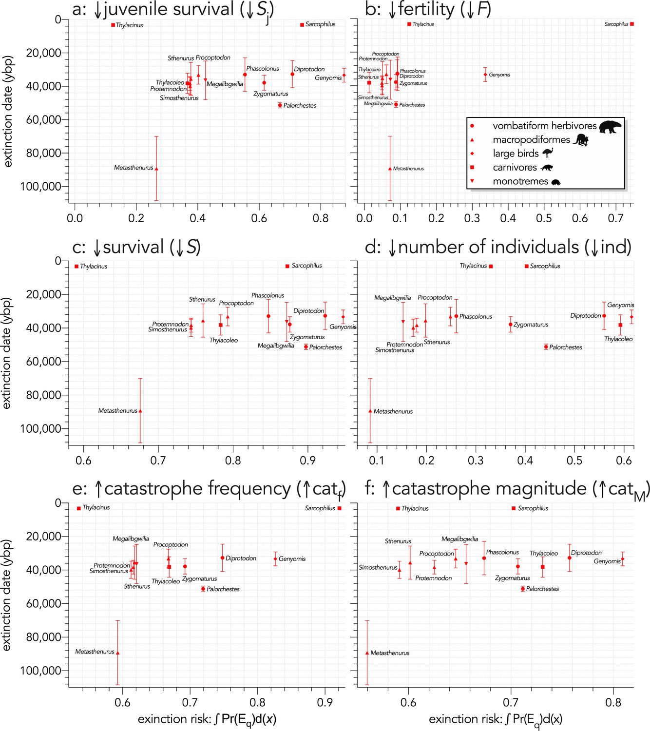
Figure 6

Relationship between estimated date of species extinction (across entire mainland) and area under the quasi-extinction curve (from Appendix 7—figure 1) — extinction risk: ∫Pr(Eq)d(x) — for (a) (Scenario ↓Sj) decreasing juvenile survival, (b) (Scenario ↓F) decreasing fertility, (c) (Scenario ↓S) decreasing survival across all age classes, (d) (Scenario ↓ind) increasing number of individuals removed year−1, (e) (Scenario ↑catf) increasing frequency of catastrophic die-offs per generation, and f: (Scenario ↑catM) increasing magnitude of catastrophic die-offs.
Extinction-timing windows are estimated based on the agreement among six different models that correct for the Signor-Lipps effect (described in Materials and methods) in chronologies of quality-rated (Rodríguez-Rey et al., 2015) fossil dates for the studied taxa described in Peters et al., 2019.
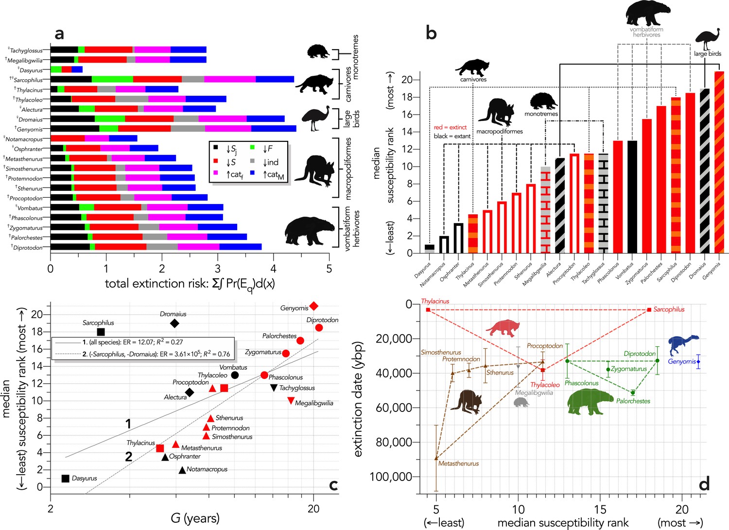
Figure 7
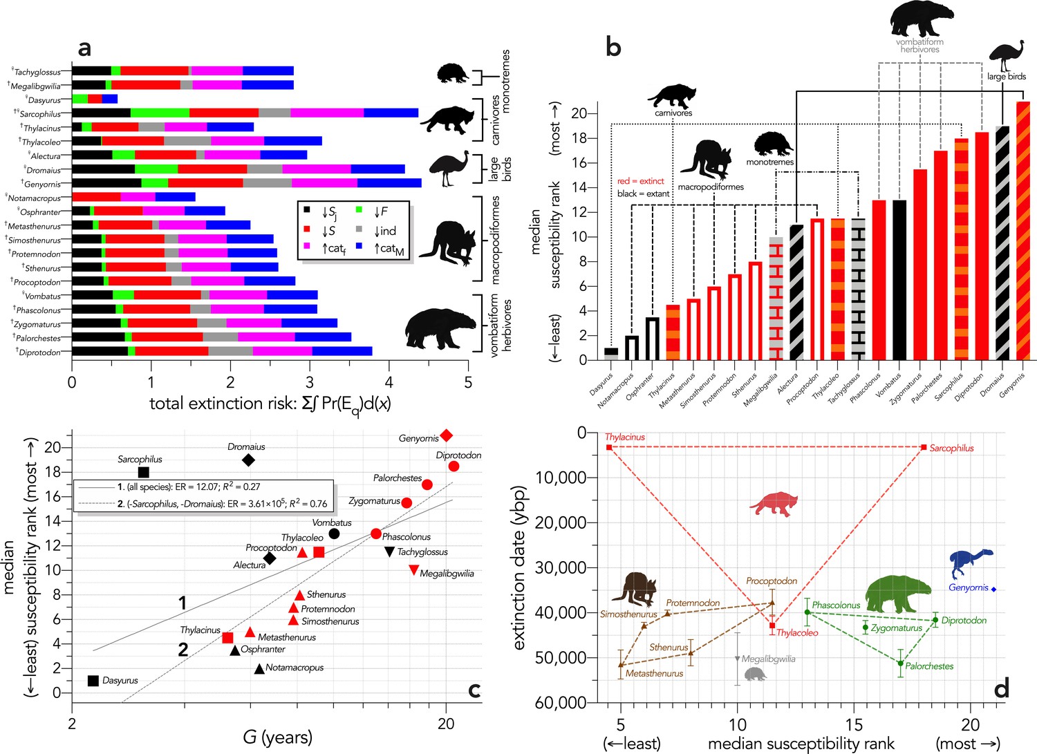
Extinction susceptibility of the 21 modelled species.
(a) Sum of the areas under the quasi-extinction curve for each of the six scenarios considered — total extinction risk: Σ∫Pr(Eq)d(x) — for each of the 21 modelled species (†extinct; ♀extant; scenario abbreviations: ↓Sj = reducing juvenile survival; ↓F = reducing fertility; ↓S = reducing survival; ind = reducing number of individuals; ↑catf = increasing frequency of catastrophe; ↑catM = increasing magnitude of catastrophe); (b) median susceptibility rank across the six scenarios considered (where higher ranks = higher susceptibility to extinction) for each species (red = extinct; black = extant; outline-only bars = macropodiformes; solid bars = vombatiforms; angled crosshatching = birds; vertical crosshatching = carnivores; brick crosshatching = monotremes); (c) median susceptibility rank as a function of log10 generation length (G, kg) — there was a weak correlation including all species (solid grey line 1), but a strong relationship removing Sarcophilus and Dromaius (dashed gray line 2) (information-theoretic evidence ratio [ER] and variance explained [R2] shown for each); (d) estimated date of species extinction (across entire continent) as a function of median susceptibility rank; taxonomic/functional groupings are indicated by coloured symbols and convex hulls (macropodids: brown; monotremes: grey; vombatiforms: green; birds: blue; carnivores: red). Extinction-timing windows are estimated based on the agreement among six different models that correct for the Signor-Lipps effect (described in Materials and methods) in chronologies of quality-rated (Rodríguez-Rey et al., 2015) fossil dates for the studied taxa described in Peters et al., 2019.
Appendix 1—figure 1
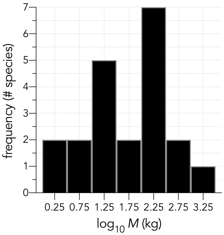
Histogram of log10 adult body masses (in kg) for the 21 species examined.
The distribution is approximately log-Normal (Shapiro-Wilk Normality test on log10M: W = 0.9804; p=0.9305).
Appendix 3—figure 1

Mass-predicted abundance and biomass for the 21 modelled species.
(a) Stable population sizes (Nstable) for each modelled species predicted from allometric estimates of population density for a 500 km × 500 km (250,000 km2) landscape (outline-only bars = macropodiformes; solid bars = vombatiforms; angled crosshatching = birds; vertical crosshatching = carnivores; brick crosshatching = monotremes); (b) Nstable plotted against body mass (M, in kg), showing the allometric scaling separating the vombatiform herbivores (green)/macropodiformes (brown), flightless birds (blue), carnivores (red), and monotremes (grey); (c) predicted landscape biomass (Nstable × M) for each species (outline-only bars = macropodiformes; solid bars = vombatiforms; angled crosshatching = birds; vertical crosshatching = carnivores; brick crosshatching = monotremes).
Here, we have depicted Sarcophilus as ‘extant’, even though it went extinct on the mainland >3000 years ago.
Appendix 5—figure 1
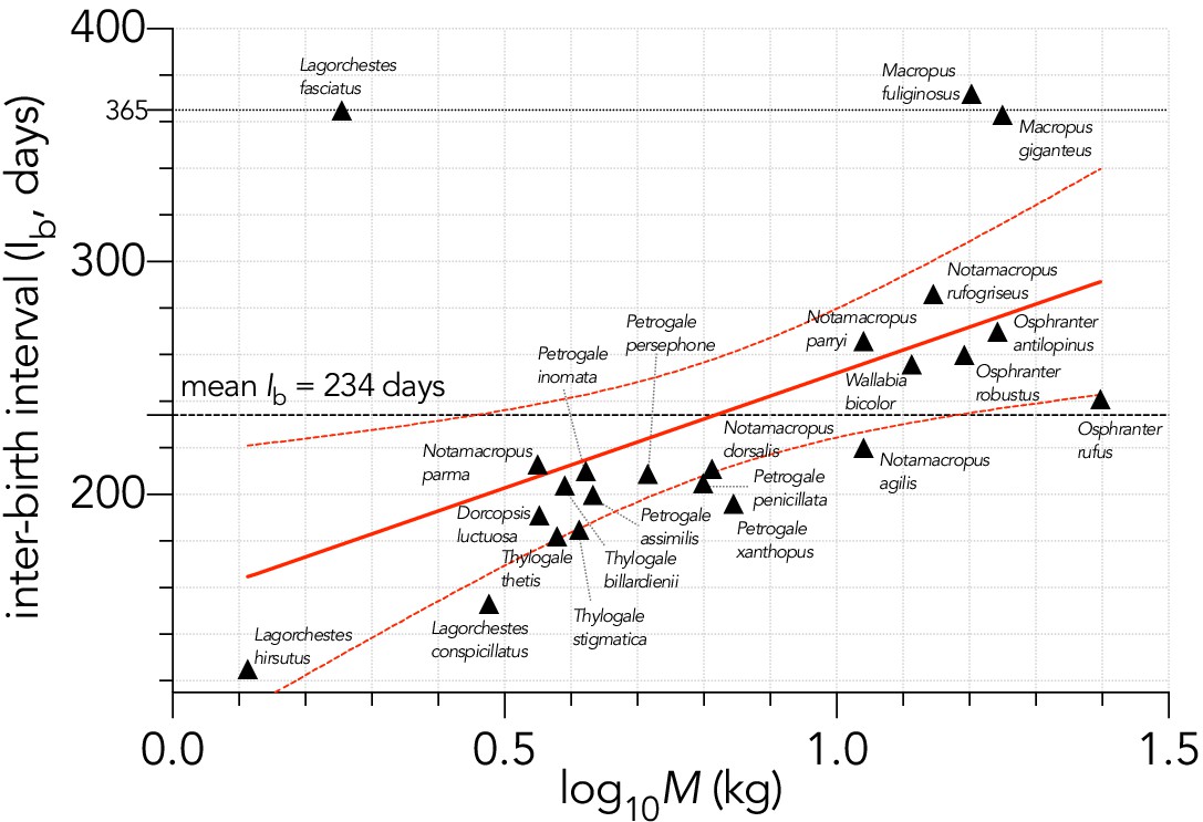
Relationship between the logarithm of adult female body mass (M, kg) and inter-birth interval (Ib, in days) for 23 extant macropodid herbivores (Fisher et al., 2001).
The estimated parameters of the linear fit (y ~ α + βx) are: α = 159.3 ± 31.5 days (± SE) and β = 93.6 ± 36.4, explaining 24.2% of the variation (), with the information-theoretic evidence ratio (ER) of the slope versus intercept-only model = 11.0.
Appendix 5—figure 2
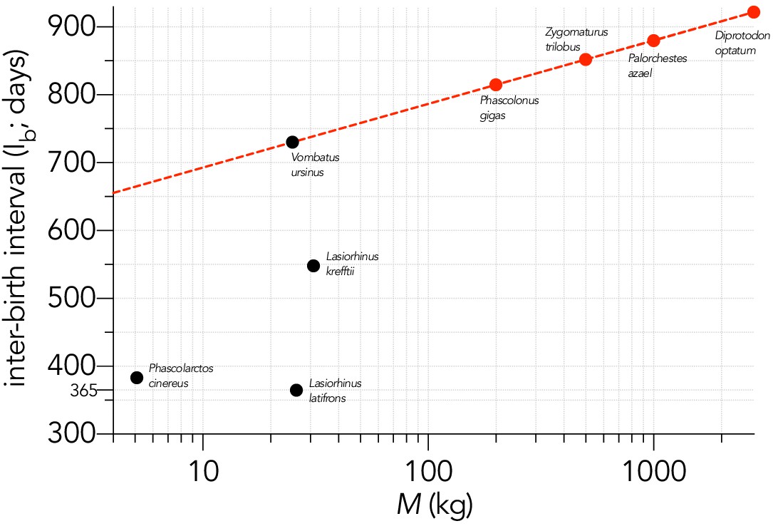
Relationship between the logarithm of adult female body mass (M, kg) and inter-birth interval (Ib, in days) for four large, extant phoscolarctid and vombatiform herbivores (black circles): koala Phascolarctos cinereus; common wombat Vombatus ursinus; northern hairy-nosed wombat Lasiorhinus krefftii; southern hairy-nosed wombat L. latifrons.
Shown is the assumed relationship between Ib and log10M setting the slope to that estimated for the extant macropodiforms (β = 93.6; Appendix 5—figure 1) and an intercept that aligned with Vombatus (α = 599 days) to estimate the inter-birth interval for the four extinct vombatiform herbivores (red circles) considered in this analysis.
Appendix 5—figure 3
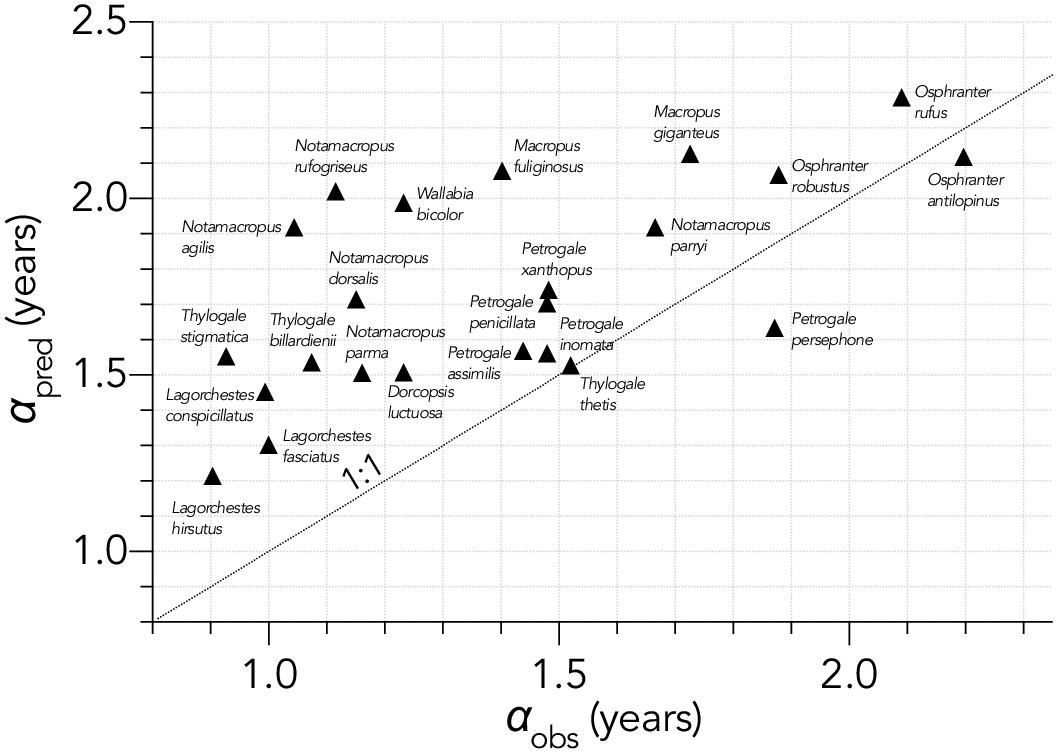
Relationship between the predicted age (years) at first breeding (αpred) and observed α (αobs) for 23 extant macropodid herbivores (Fisher et al., 2001).
The allometric prediction over-estimated α by and average of ~20%. Also shown is the 1:1 line (dashed).
Appendix 5—figure 4

Negative relationship between the logarithm of the maximum rate of intrinsic population growth (log10rm) and the logarithm of the age at primiparity (log10α) for the 21 species examined.
The estimated parameters of the linear fit (y ~ α + βx) including all species (black lines) are: α = -0.388 ± 0.075 (± SE) and β = -0.931 ± 0.146, and explaining 66.4% of the variation (), with the information-theoretic evidence ratio (ER) of the slope versus intercept-only model = 4.052×10⁴. This relationship is similar to the theoretical expectation for the intercept = -0.15 and slope = -1.0 for mammals (Hone et al., 2010). Birds (Alectura, Dromaius, Genyornis; ◆) potentially fall outside this relationship, so just considering the remaining mammals (●), the parameters for the linear fit (red lines) become: α = -0.388 ± 0.083 (± SE), β = -0.875 ± 0.170, = 60.1%, and ER = 1.567×10³.
Appendix 6—figure 1
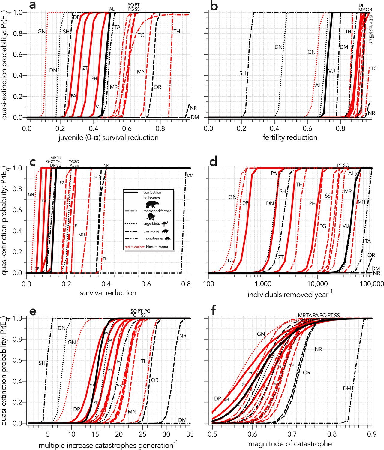
Increasing probabilities of quasi-extinction — quasi-extinction probability: Pr(Eq) — as a function of (a) decreasing juvenile survival (Scenario ↓Sj), (b) decreasing fertility (Scenario ↓F), (c) decreasing survival across all age classes (Scenario ↓S), (d) increasing number of individuals removed year−1 (Scenario ↓ind), (e) increasing frequency of catastrophic die-offs per generation (Scenario ↑catf), and (f) increasing magnitude of catastrophic die-offs (Scenario ↑catM).
Species notation: DP = Diprotodon optatum, PA = Palorchestes azael, ZT = Zygomaturus trilobus, PH = Phascolonus gigas, VU = Vombatus ursinus (vombatiform herbivores); PG = Procoptodon goliah, SS = Sthenurus stirlingi, PT = Protemnodon anak, SO = Simosthenurus occidentalis, MN = Metasthenurus newtonae, OR = Osphranter rufus, NR = Notamacropus rufogriseus (macropodiformes); GN = Genyornis newtoni, DN = Dromaius novaehollandiae, AL = Alectura lathami (large birds); TC = Thylacoleo carnifex, TH = Thylacinus cynocephalus, SH = Sarcophilus harrisii, DM = Dasyurus maculatus (carnivores); TA = Tachyglossus aculeatus, MR = Megalibgwilia ramsayi (monotreme invertivores). Here, we have depicted SH as ‘extant’, even though it went extinct on the mainland >3000 years ago.
Appendix 7—figure 1
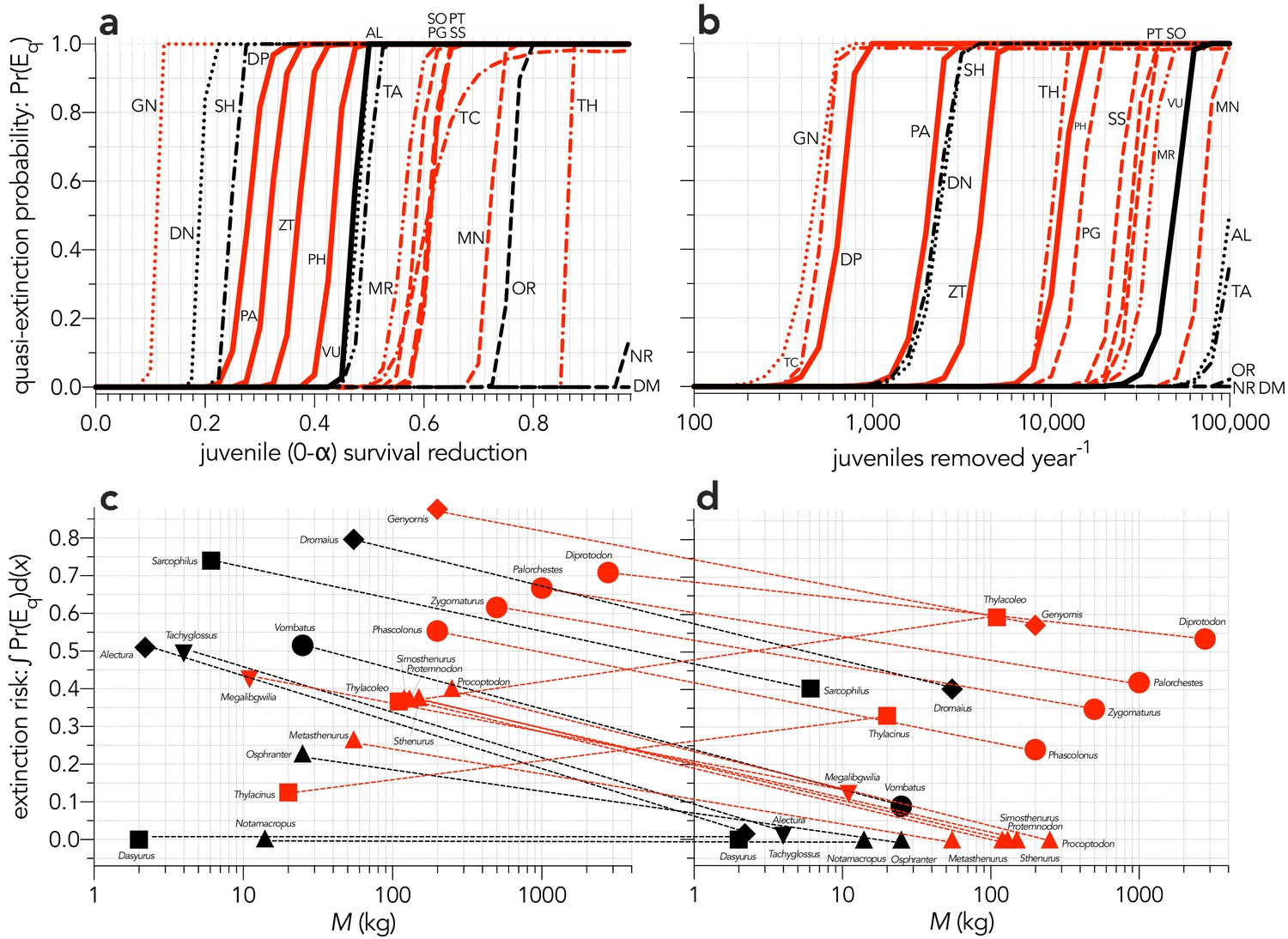
Increasing probabilities of quasi-extinction — quasi-extinction probability: Pr(Eq) — as a function of (a) decreasing juvenile survival (Scenario ↓Sj), and (b) increasing number of juvenile individuals removed year−1 (Scenario ↓indj).
Also shown is the corresponding area under the quasi-extinction curve — extinction risk: ∫Pr(Eq)d(x) — as a function body mass for (c) increasing juvenile mortality and (d) increasing number of juvenile individuals removed year−1. The dashed lines in c and d indicate the change in relative susceptibility between scenarios. Species notation: DP = Diprotodon optatum, PA = Palorchestes azael, ZT = Zygomaturus trilobus, PH = Phascolonus gigas, VU = Vombatus ursinus (vombatiform herbivores); PG = Procoptodon goliah, SS = Sthenurus stirlingi, PT = Protemnodon anak, SO = Simosthenurus occidentalis, MN = Metasthenurus newtonae, OR = Osphranter rufus, NR = Notamacropus rufogriseus (macropodiformes); GN = Genyornis newtoni, DN = Dromaius novaehollandiae, AL = Alectura lathami (large birds); TC = Thylacoleo carnifex, TH = Thylacinus cynocephalus, SH = Sarcophilus harrisii, DM = Dasyurus maculatus (carnivores); TA = Tachyglossus aculeatus, MR = Megalibgwilia ramsayi (monotreme invertivores). Red = extinct; black = extant. Here, we have depicted SH as ‘extant’, even though it went extinct on the mainland >3000 years ago.
Appendix 8—figure 1
Relationship between estimated date of species extinction (across the entire continent) based on a jack-knifed GRIWM approach (Bradshaw et al., 2012; Saltré et al., 2015) and (a) body mass (kg) or (b) generation length (years) (Scenario LH).
Extinction-timing windows are estimated based on the agreement among six different models that correct for the Signor-Lipps effect (described in Materials and methods) in chronologies of quality-rated (Rodríguez-Rey et al., 2015) fossil dates for the studied taxa described in Peters et al., 2019. Here, we have depicted Sarcophilus as ‘extant’, even though it went extinct on the mainland >3000 years ago. Also shown are the approximate major climate periods and transitions: Marine Isotope Stage 5 (MIS 5), MIS 4, MIS 3, MIS 2 (including the Last Glacial Maximum, Antarctic Cold Reversal, and Younger Dryas), and the Holocene (including the period of sea level flooding when Tasmania separated from the mainland, and the relatively warm, wet, and climatically stable Holocene optimum).
Appendix 8—figure 2
Relationship between estimated date of species extinction (across the entire mainland) based on a jack-knifed GRIWM approach (Bradshaw et al., 2012; Saltré et al., 2015) and area under the quasi-extinction curve (from Fig. S7) — extinction risk: ∫Pr(Eq)d(x) — for (a) (Scenario ↓Sj) decreasing juvenile survival, (b) (Scenario ↓F) decreasing fertility, (c) (Scenario ↓S) decreasing survival across all age classes, (d) (Scenario ↓ind) increasing number of individuals removed year−1, (e) (Scenario ↑catf) increasing frequency of catastrophic die-offs per generation, and (f) (Scenario ↑catM) increasing magnitude of catastrophic die-offs.
Extinction-timing windows are estimated based on the agreement among six different models that correct for the Signor-Lipps effect (described in Materials and methods) in chronologies of quality-rated (Rodríguez-Rey et al., 2015) fossil dates for the studied taxa described in Peters et al., 2019.
Appendix 8—figure 3
(a) Sum of the areas under the quasi-extinction curve for each of the six scenarios considered — total extinction risk: Σ∫Pr(Eq)d(x) — for each of the 21 modelled species (†extinct; ♀extant; scenario abbreviations: ↓Sj = reducing juvenile survival; ↓F = reducing fertility; ↓S = reducing survival; ind = reducing number of individuals; ↑catf = increasing frequency of catastrophe; ↑catM = increasing magnitude of catastrophe); (b) median susceptibility rank across the six scenarios considered (where higher ranks = higher susceptibility to extinction) for each species (red = extinct; black = extant; outline-only bars = macropodiformes; solid bars = vombatiforms; angled crosshatching = birds; vertical crosshatching = carnivores; brick crosshatching = monotremes); (c) median susceptibility rank as a function of log10 generation length (G, kg) — there was a weak correlation including all species (solid grey line 1), but a strong relationship after removing Sarcophilus and Dromaius (dashed grey line 2) (information-theoretic evidence ratio [ER] and variance explained [R2] shown for each); (d) estimated date of species extinction (across entire continent) as a function of median susceptibility rank; taxonomic/functional groupings are indicated by colored symbols and convex hulls (macropodids: brown; monotremes: grey; vombatiforms: green; birds: blue; carnivores: red).
Extinction-timing windows are on a jack-knifed GRIWM approach (Bradshaw et al., 2012; Saltré et al., 2015) that corrects for the Signor-Lipps effect in chronologies of quality-rated (Rodríguez-Rey et al., 2015) fossil dates for the studied taxa described in Peters et al., 2019.
Appendix 9—figure 1
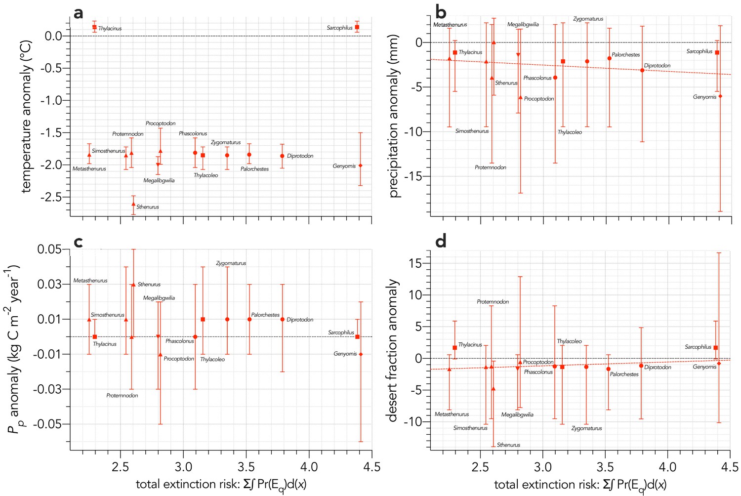
Sum of the areas under the quasi-extinction curve over the six scenarios considered — total extinction risk: Σ∫Pr(Eq)d(x) — for each of the 13 extinct (mainland only) modelled species relative to (a) mean annual temperature anomaly (°C): information-theoretic evidence ratio of the slope model relative to the intercept-only model (ERmean) = 0.75 for the mean climate values; probability of a non-random slope relationship incorporating full uncertainty in the climate variable pu = 0.603.
(b) mean annual precipitation anomaly (mm): ERmean = 9.6; pu = 0.461. (c) net primary production anomaly (kg C m−2 year−1): ERmean <0.01; pu = 0.411. (d) desert fraction anomaly: ERmean = 4.2; pu = 0.425. The dashed red line in panels a, b, and d indicate evidence for a slope model versus the intercept-only model for these variables (ERmean >2). Error bars indicate ±1 standard deviation.
Tables
Appendix 2—table 1
Predicted demographic values for each species (equations provided in Materials and methods and this appendix).
M = mass, rm = maximum rate of instaneous exponential population growth predicted allometrically, = realised rm predicted from the constructed matrix (see text), ω = longevity, F = fertility (daughters per breeding female per year), α = age at first reproduction (primiparity), Sad = yearly adult survival, G = generation length. †extinct; ♀extant. See Appendix 2—table 2 for rank correlations among demographic values across species.
| Species | M (kg) | rm | D (km−2) | ω (yrs) | F (n♀yr−1♀−1) | α (yrs) | Sad (yr−1) | G (yrs) | |
|---|---|---|---|---|---|---|---|---|---|
| vombatiform herbivores | |||||||||
| Diprotodon† | 2786 | 0.100 | 0.061 | 0.134 | 48 | 0.1311 | 7 | 0.985 | 18.1 |
| Palorchestes† | 1000 | 0.131 | 0.077 | 0.285 | 42 | 0.1705 | 6 | 0.981 | 15.1 |
| Zygomaturus† | 500 | 0.157 | 0.095 | 0.476 | 39 | 0.2038 | 5 | 0.977 | 13.2 |
| Phascolonus† | 200 | 0.200 | 0.121 | 0.938 | 34 | 0.2586 | 4 | 0.972 | 10.7 |
| Vombatus♀ | 25 | 0.345 | 0.119 | 4.370 | 26 | 0.2500 | 2 | 0.953 | 10.0 |
| macropodiform herbivores | |||||||||
| Proctoptodon† | 250 | 0.189 | 0.188 | 0.795 | 17 | 0.524 | 3 | 0.973 | 8.3 |
| Sthenurus† | 150 | 0.216 | 0.215 | 1.161 | 17 | 0.617 | 3 | 0.970 | 8.1 |
| Protemnodon† | 130 | 0.224 | 0.224 | 1.290 | 16 | 0.646 | 3 | 0.969 | 7.8 |
| Simosthenurus† | 120 | 0.229 | 0.226 | 1.369 | 16 | 0.663 | 3 | 0.968 | 7.8 |
| Metasthenurus† | 55 | 0.281 | 0.280 | 2.438 | 14 | 0.858 | 2 | 0.961 | 6.0 |
| Osphranter♀ | 25 | 0.345 | 0.343 | 4.370 | 13 | 0.750 | 2 | 0.953 | 5.5 |
| Notamacropus♀ | 14 | 0.402 | 0.351 | 6.712 | 16 | 0.668 | 1 | 0.993 | 6.3 |
| large birds | |||||||||
| Genyornis† | 200 | 0.041 | 0.041 | 0.101 | 38 | 0.658 | 9 | 0.987 | 20.0 |
| Dromaius♀ | 55 | 0.100 | 0.100 | 0.290 | 17 | 1.938 | 3 | 0.983 | 5.9 |
| Alectura♀ | 2.2 | 0.176 | 0.175 | 3.633 | 27 | 7.188 | 2 | 0.967 | 6.8 |
| carnivores | |||||||||
| Thylacoleo† | 110 | 0.234 | 0.201 | 0.028 | 14 | 0.500 | 4 | 0.967 | 9.1 |
| Thylacinus† | 20 | 0.366 | 0.368 | 0.159 | 10 | 1.556 | 1 | 0.950 | 5.2 |
| Sarcophilus†,♀ | 6.1 | 0.500 | 0.094 | 0.539 | 5 | 1.205 | 1 | 0.820 | 3.1 |
| Dasyurus♀ | 2.0 | 0.701 | 0.644 | 2.023 | 4 | 1.582 | 1 | 0.910 | 2.3 |
| monotremes | |||||||||
| Megalibgwilia† | 11.0 | 0.307 | 0.107 | 3.522 | 51 | 0.222 | 3 | 0.977 | 16.4 |
| Tachyglossus♀ | 4.0 | 0.400 | 0.112 | 9.883 | 45 | 0.275 | 3 | 0.950 | 14.1 |
-
Sarcophilus harrisii is extinct in mainland Australia, but extant in the island state of Tasmania.
Thylacinus could also be treated like Sarcophilus in that Thylacinus survived in Tasmania until historical times (1930s).
-
In the case of the vombatiform and macropodiform herbivores, ω shown in the table is in fact the downscaled ω′ calculated for each group (see below). Likewise, both allometric predictions of F and α are corrected for these groups (see Supplementary Information Appendix 5).
Appendix 2—table 2
Kendall’s rank correlation (τ) among demographic values given in Appendix 2—table 1 across species.
M = mass, rm = maximum rate of instaneous exponential population growth predicted allometrically, = realised rm predicted from the constructed matrix (see text), ω = longevity, F = fertility (daughters per breeding female per year), α = age at first reproduction (primiparity), Sad = yearly adult survival, G = generation length.
| M (kg) | rm | rm' | D (km−2) | ω (yrs) | F (n♀yr−1♀−1) | α (yrs) | Sad (yr−1) | |
|---|---|---|---|---|---|---|---|---|
| rm | −0.684 | |||||||
| rm' | −0.350 | 0.507 | ||||||
| D (km−2) | −0.476 | 0.499 | 0.358 | |||||
| ω (yrs) | 0.390 | −0.511 | −0.605 | −0.068 | ||||
| F (n♀yr−1♀−1) | −0.484 | 0.278 | 0.486 | 0.148 | −0.567 | |||
| α (yrs) | 0.671 | −0.685 | −0.583 | −0.459 | 0.556 | −0.562 | ||
| Sad (yr−1) | 0.552 | −0.681 | −0.394 | −0.328 | 0.484 | −0.327 | 0.572 | |
| G (yrs) | 0.471 | −0.446 | −0.616 | −0.201 | 0.762 | −0.711 | 0.730 | 0.487 |
Additional files
Download links
A two-part list of links to download the article, or parts of the article, in various formats.
Downloads (link to download the article as PDF)
Open citations (links to open the citations from this article in various online reference manager services)
Cite this article (links to download the citations from this article in formats compatible with various reference manager tools)
Relative demographic susceptibility does not explain the extinction chronology of Sahul’s megafauna
eLife 10:e63870.
https://doi.org/10.7554/eLife.63870


