Mesoscale phase separation of chromatin in the nucleus
- Weizmann Institute of Science, Israel
Figures
Figure 1 with 1 supplement
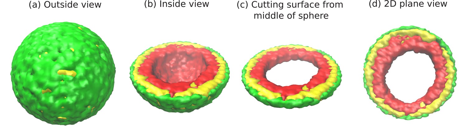
Snapshots of the simulated system from different views.
This representation is generated by drawing the surfaces around the beads that represent the lamin and chromatin. The same set of pictures shown here are depicted in a different graphical representation, in terms of the beads themselves, in Figure 1—figure supplement 1. (a) Outside view: Our model, spherical nucleus is enclosed by lamin (NL) beads (green). Within the sphere, the chromatin chain of N = 37,333 beads contains two types of beads: LAD (yellow) and non-LAD (red). (b) Inside view: The sphere is cut at the equatorial plane to reveal one hemisphere, so that chromatin (red and yellow) is visible. The central region of the nucleus is devoid of chromatin for the particular conditions () of this simulation. (c) Cutting a slice near the equatorial plane: A slice is cut from the hemisphere, resulting in a 3D surface which has width of of the sphere diameter. (d) 2D planar view: We show the equatorial (xy) plane view of the 3D slice and observe that the central regions contains no chromatin.
Figure 1—figure supplement 1
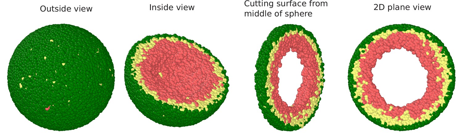
Snapshots of the simulated system visualized in terms of beads.
Outside view: The spherical volume representing the nucleus is surrounded by lamin beads (green). Within the sphere, the chromatin chain of N = 37,333 beads comprises two types beads: LAD (yellow) and non-LAD (red). Inside view: Spherical system is cut at the equatorial plane into two hemispheres, so that chromatin (LAD: yellow beads, non-LAD: red beads) within one hemisphere is visible. Section cut from the equatorial plane of the hemisphere: Sphere is cut from its equatorial plane into a slice with a width of (1/5)th of sphere diameter. 2D plane view: We show the equatorial (xy) plane view of the 3D surface where it is clear that there is no chromatin in the middle which is filled with the aqueous phase.
Figure 2
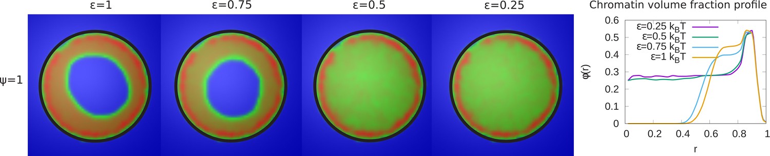
Variation of the chromatin concentration profile as a function of the intra-chromatin attractive interactions.
Left panel: Chromatin concentrations are shown for different intra-chromatin attraction strengths () with a volume fraction of chromatin and maximal LAD-lamina interactions (). For smaller values of the attractions, the chromatin no longer shows peripheral localization, and fills the entire nucleus. This demonstrates the role of the chromatin self-attractions in stabilizing peripheral chromatin organization with a relatively high local volume fraction (red) of chromatin compared to the case of relatively small self-attractions where the chromatin fills the entire nucleus, with a smaller local volume fraction (green). Right panel: The local volume fraction profiles of chromatin for different plotted as a function of the radial distance where is the nuclear center and is the position of the nuclear envelope. These local volume fraction profiles are obtained by averaging over the azimuthal and polar angles in thin spherical shells at distances from the nuclear center to the nuclear periphery.
Figure 3 with 1 supplement
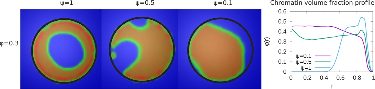
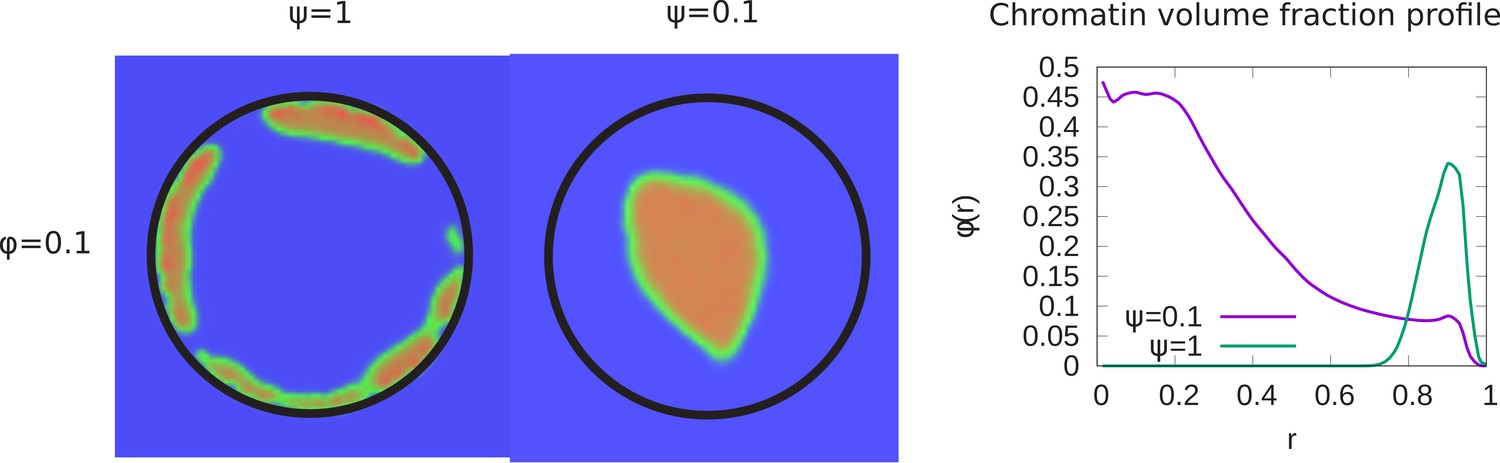
Variation of the chromatin concentration profile as a function of the fraction of LAD domains bound to the lamina.
Left panel: Variation in the fraction ψ of LAD beads that can bond to the lamin, associated domains relative to its maximal value of , where 48% of the chromatin consists of LAD domains that can bind to the lamin. The values of the chromatin volume fraction and chromatin self-interaction strength, are fixed. Those LAD domains (a fraction, ) not bound to the lamin are not necessarily found near the periphery of the nucleus and are mixed with the non-LAD chromatin. For small values of ψ, the chromatin is no longer peripherally localized but fills the nucleus more uniformly (but see the discussion of the ‘wetting droplet’ in Appendix 5 and Appendix 5—figure 1), since there are relatively few LAD-lamin bonds to localize the chromatin at the nuclear periphery. Right panel: The local volume fraction profiles of chromatin as a function of the radial distance , where is the nuclear center and is the location of the nuclear envelope.
Figure 3—figure supplement 1
Transition from peripheral to central chromatin localization.
Here we show the transition from peripheral to central chromatin localization for small chromatin volume fraction as the fraction of chromatin that can bind to the lamin is varied from to . Left panel: For a small chromatin volume fraction , simulation snapshots show peripheral chromatin localization for and central localization (but see the next section on the wetting droplet) for . Right panel: Local chromatin volume fraction shows a peak near the nuclear periphery () for while for , the peak of the local volume fraction is shifted toward the center ().
Figure 4
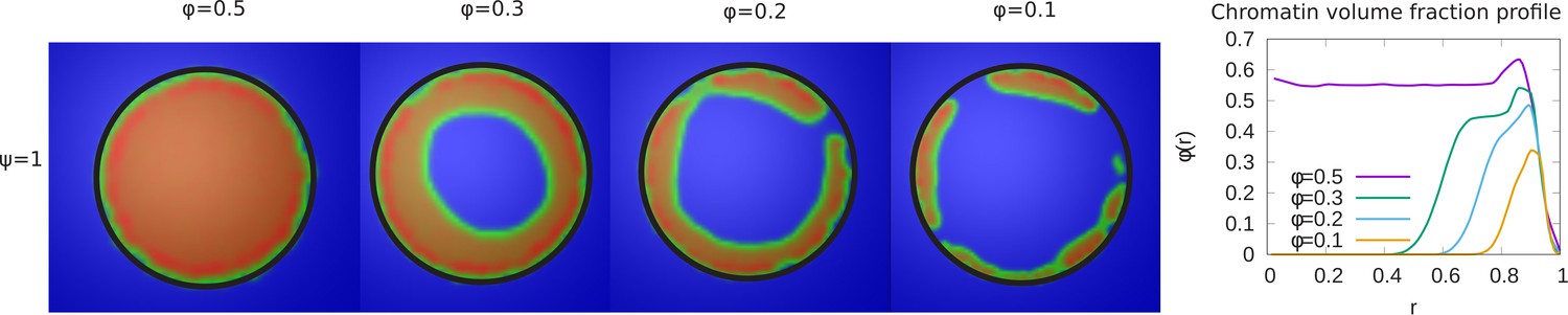
Variation of the chromatin concentration profile as a function of the chromatin volume fraction.
Left panel: Chromatin concentrations are shown for different volume fractions of chromatin, . Right panel: The local volume fraction profiles show peripheral organization for and but not for . This demonstrates the transition from peripheral to conventional chromatin organization as the nucleus is dehydrated and is increased.
Figure 5

State diagrams showing the transition from peripheral to uniform to central localization of chromatin.
(a) For a fixed value of (maximally bonded LAD), we calculated the local volume fraction obtained from simulations with different pairs (24 pairs) of the chromatin volume fraction and self-attraction where and . For each pair of , we used the plots of the local volume fraction to determine the chromatin organization mode. In the graph, the blue line shows the transition between conventional (uniformly distributed) chromatin organization, and peripheral organization. (b) For a fixed value of the chromatin self-attraction , we calculated the local volume fraction obtained from simulations with different pairs (60 pairs) of the chromatin volume fraction and fraction of LAD that can bond to the lamina where and . The blue line shows the transition from central (and wetting drop) to peripheral chromatin organization. In figures (a) and (b), the bars are the simulation results while the line is a guide to the eye.
Figure 6

Angular separation of LAD and non-LAD chromatin.
(a) Simulation snapshot for parameter values , , and , shows peripheral organization with LAD near lamina and non-LADs separated from LADs in the radial direction. (b) Simulation snapshot for parameter values , , and , shows peripheral organization with alternating LAD and non-LAD regions in the angular direction at the nuclear periphery. (c) Experimentally labeled H3K9ac (euchromatin/most of non-LAD/green) and His2B (chromatin/LAD and non-LAD/red) in muscle nuclei of intact Drosophila larvae, shows heterochromatin (associated with LAD) by dark red color and euchromatin (associated with non-LAD) by merging the red and green colors in peripheral organization. Both the experiments and simulations show an angular distribution of LAD and non-LAD as opposed to a radial distribution.
Appendix 1—figure 1
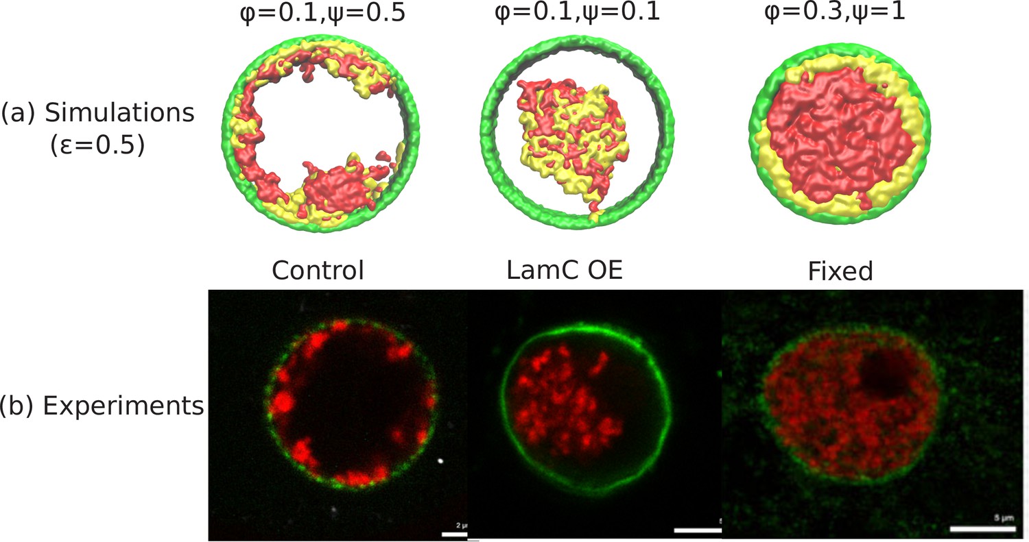
Comparison of the simulations with the experimental images.
(a) Snapshots of simulations for chromatin-chromatin attractions . For relatively small volume fraction of chromatin () and relatively high chromatin-lamina binding interactions (), the simulation shows peripheral organization of chromatin. For (small) and (small), we obtain central organization of chromatin (see Appendix 5 on the wetting droplet). For (high) and (high), the simulations show conventional organization of chromatin, where the entire nucleus is filled. (b) Different organization of chromatin obtained in the experiments: peripheral, central and conventional are seen in experiments in the control, lamin A/C overexpression and fixed nuclei respectively (Amiad-Pavlov et al., 2020).
Appendix 2—figure 1
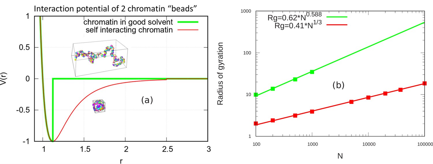
Scaling behavior of unconfined chromatin chains in good and poor solvent.
(a) LJ potential as a function of the distance between two beads, with snapshot of simulations of chromatin chain having 500 beads. Snapshots show unconfined, self-avoiding chromatin in good solvent conditions for a cutoff distance (green) and self-attractive chromatin in poor solvent conditions, for a cutoff distance . (b) Radius of gyration vs. the number of beads is calculated from the simulations of unconfined chromatin chain having beads (green and red dots). The green and red lines are guides to the eye. They can be fit with the power laws shown, demonstrating the polymeric scaling in the unconfined case for both good and poor solvent conditions.
Appendix 3—figure 1
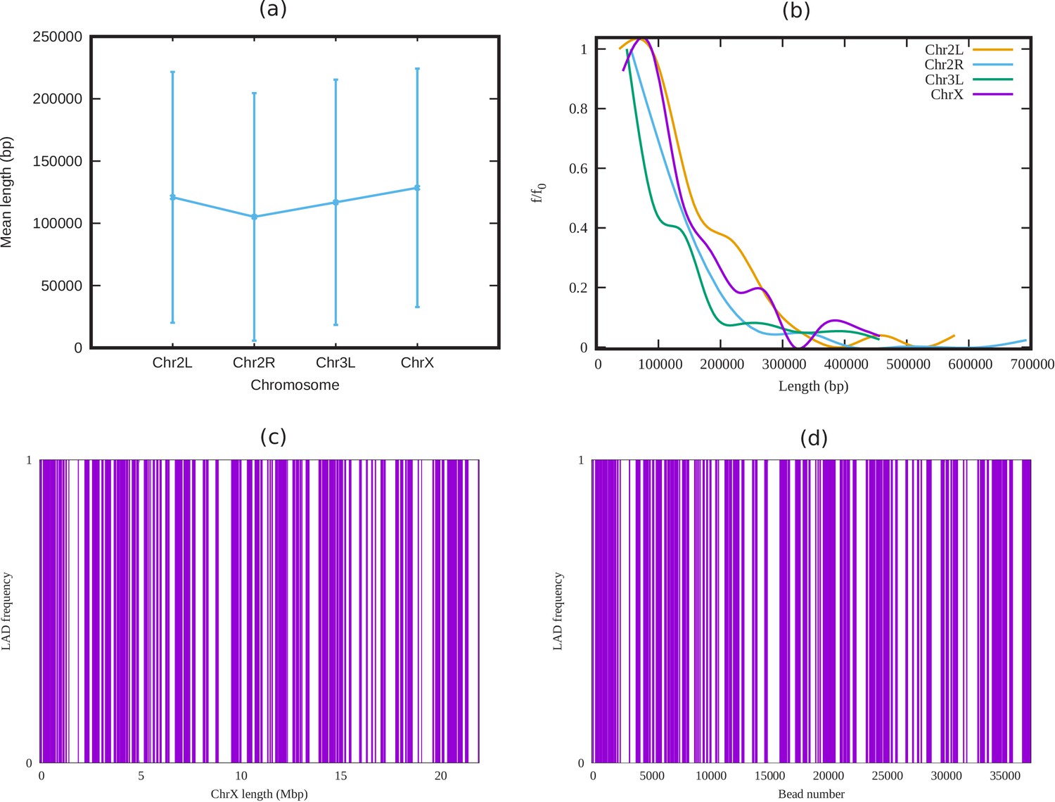
Analysis of LADs sequence data of Drosophila.
(a) Mean cluster length of LAD for different chromosomes of Drosophila (Ho et al., 2014). (b) Length distribution of LAD for different Drosophila chromosomes. In both subfigures (a) and (b), the vertical bars represent the standard deviation (SD). (c) An alternating distribution of LAD (violet) and non-LAD (white) along the 22.4 Mbp regions of chromosome X (ChrX). (d) Same LAD distribution used in our coarse-grain model with a chromatin chain of 37,333 beads. From the sequence data it is clear, LAD regions in Drosophila consist of beads, and not single ones.
Appendix 4—figure 1
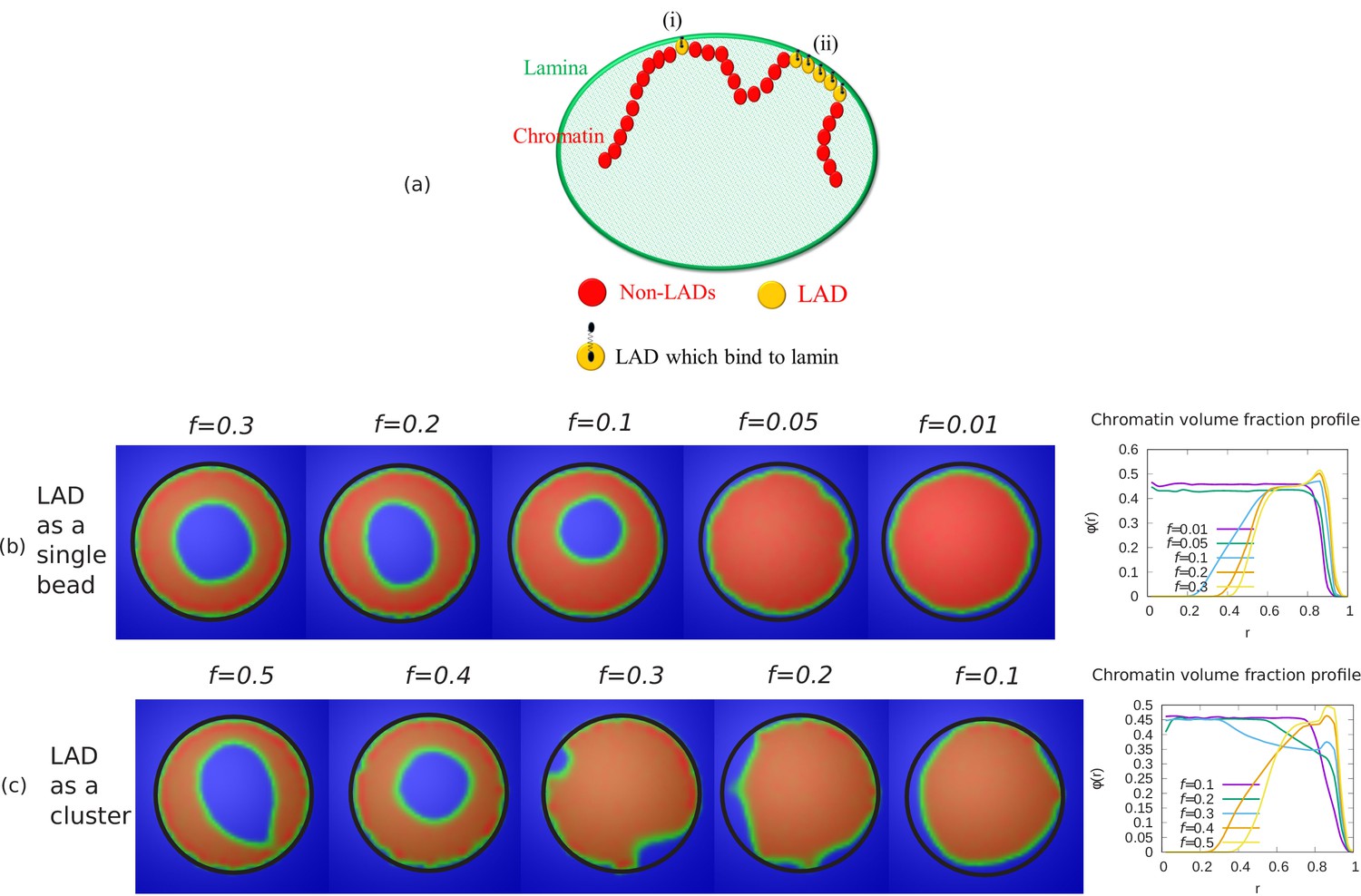
Alternate simulations for random LAD sequences.
(a) Schematic diagram describing our coarse-grained model of chromatin-lamina interactions. Two cases for LAD binding to lamin: (i) Randomly distributed as single beads, (ii) Exponentially distributed cluster (many beads). Chromatin concentrations and local chromatin volume fraction profiles for and are shown when LAD binds to lamin as a (b) single bead (c) cluster.
Appendix 4—figure 2
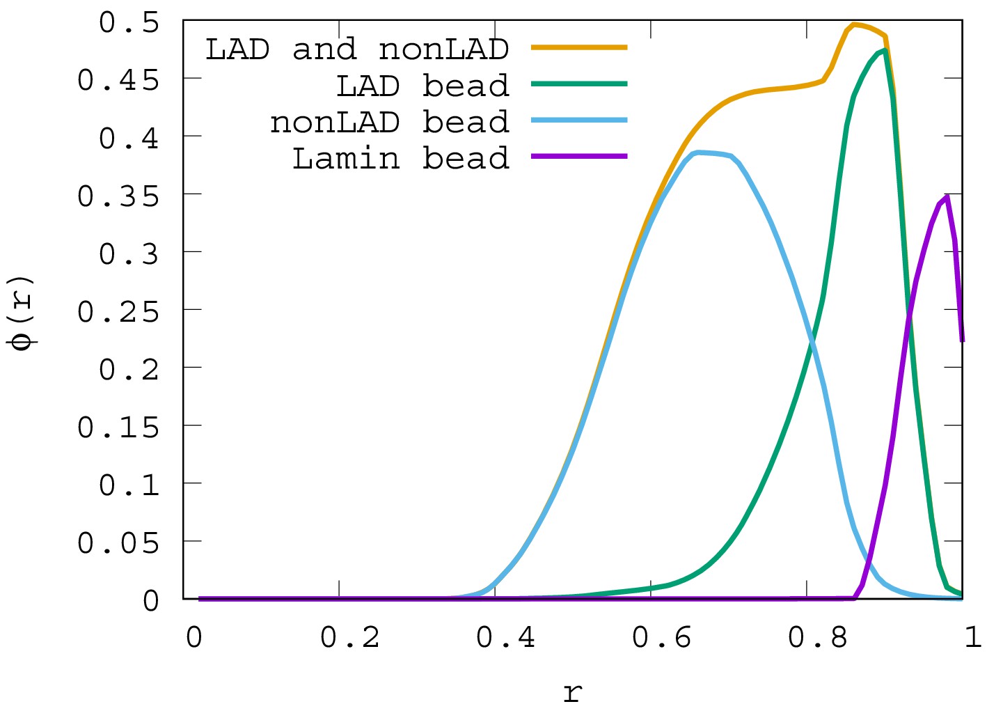
Local volume fraction profiles of LAD, non-LAD, and lamin beads.
For , the local volume fraction profiles of LAD, non-LAD and lamin beads are shown. The graph shows the location of each of these bead types in the spherical volume where is the sphere center and is the sphere surface.
Appendix 5—figure 1
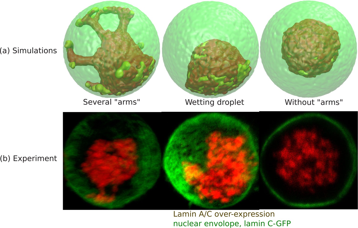
Wetting droplet and central chromatin organization for relatively weak LAD-lamina interactions.
(a) 3D snapshots of simulations showing central organization of chromatin with/without ‘arms’ as well as the wetting droplet. (b) Experiments also suggest central organization of chromatin with/without ‘arms’ as well as the wetting droplet for the case of Lamin A/C overexpression (Amiad-Pavlov et al., 2020).
Appendix 6—figure 1
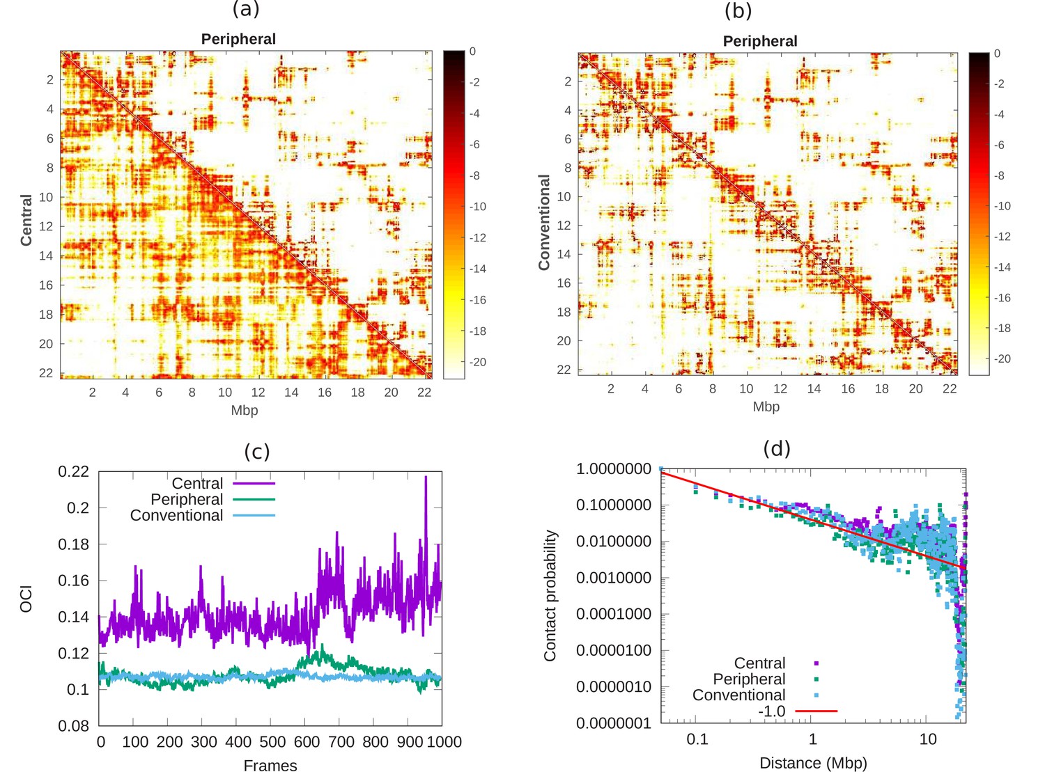
Comparison of chromatin contacts in peripheral, central, and conventional organization.
(a,b) Contact maps from simulations, of different 50-kbp bins, for different chromatin organization. The color scheme varies from black to white, representing high to low contact counts (). (a) Comparison of contact map of central (lower diagonal) and peripheral (upper diagonal) chromatin organization. (b) Comparison of contact map of conventional (lower diagonal) and peripheral (upper diagonal) chromatin organization. (c) Open chromatin index (OCI) plotted with respect to time (simulation frames) for central, peripheral, and conventional organization chromatin. (d) Contact probability as a function of contour distance for central, peripheral, and conventional organization chromatin, calculated from the simulations (dots). The red line is a guide to the eye indicating a power-law behavior, which suggests the fractal globule packing nature.
Appendix 7—figure 1
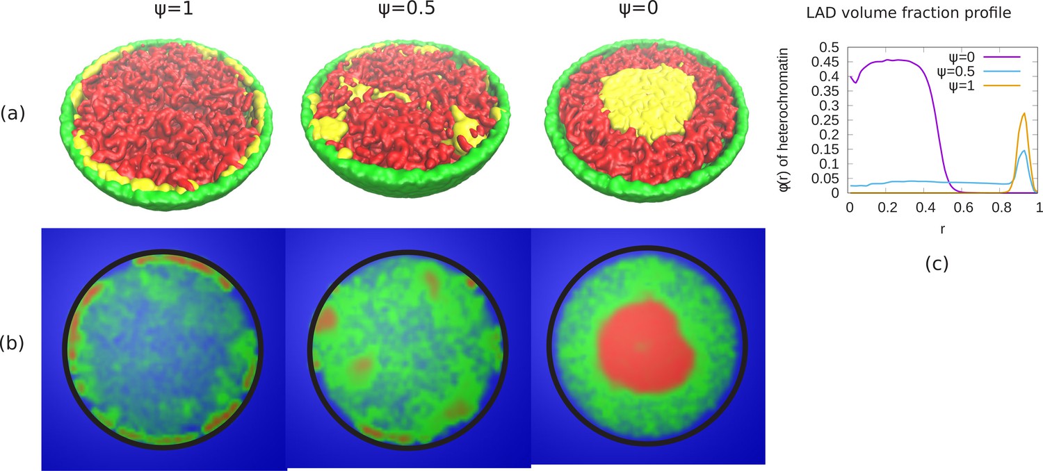
Phase separation of euchromatin-like and heterochromatin-like regions in conventional chromatin.
(a) Snapshots of simulations for different ψ are shown. In figure, LAD beads (yellow) are self attractive chain whereas non-LAD beads (red) are self-avoiding. This modeling results in a stronger separation of the two types of beads into spatially distinct regions. (b) Chromatin concentrations for different ψ are shown. High (red) and low (green) concentrations of chromatin with aqueous phase (blue) shows A/B compartments like (non-uniform) distribution of chromatin. (c) Local volume fraction of the LAD beads shows peripheral organization of those regions for , a uniform distribution for and central organization for .
Tables
Table 1
Parameter values used in the simulations.
| Parameter | Description | Reduced unit | SI unit |
|---|---|---|---|
| Thermal energy | 1.0 | 4.1 × 10⁻²¹J | |
| Bead mass | 1.0 | 10−21 kg | |
| σ | LJ size parameter | 1.0 | 10 nm |
| LJ energy parameter | 4.1 × 10⁻²¹J | ||
| rc | Contact distance | 25 nm | |
| ks | Spring constant | 0.41 Jm−2 | |
| lp | Persistence length | 20 nm | |
| kb | Bending stiffness | 8.2 × 10⁻²¹J | |
| τ | Damping time | 2 µs | |
| Time step | 20 ns |
Additional files
Download links
A two-part list of links to download the article, or parts of the article, in various formats.
Downloads (link to download the article as PDF)
Open citations (links to open the citations from this article in various online reference manager services)
Cite this article (links to download the citations from this article in formats compatible with various reference manager tools)
Mesoscale phase separation of chromatin in the nucleus
eLife 10:e63976.
https://doi.org/10.7554/eLife.63976


