The neural basis of intelligence in fine-grained cortical topographies
- Center for Cognitive Neuroscience, Dartmouth College, United States
- Vicarious AI, United States
Figures
Figure 1

Schematic illustration of coarse- and fine-grained functional connectivity.
Each brain region (e.g., area 150 shown here) comprises multiple cortical vertices (on average 165). Correlations between their time series and time series for all 59,412 vertices in the whole cortex form that region’s full fine-grained connectivity matrix (top row). The fine-grained connectivity profiles for 360 brain regions each have approximately 10 million such correlations. The coarse-grained connectivity profile for the same region (middle row) comprises the average functional connectivity between all of the vertices in that region and all of the vertices in each of the 360 brain regions. Thus, the coarse-grained connectivity profiles for 360 brain regions each have 360 mean correlations. The residual fine-grained connectivity profile (bottom row) for each region is obtained by subtracting the mean correlation for a pair of regions (e.g., regions 1 and 150) from the full fine-grained connectivity profile for that pair and is, thus, unconfounded with coarse-grained functional connectivities. We refer to these unconfounded profiles as fine-grained connectivity profiles for short.
Figure 2
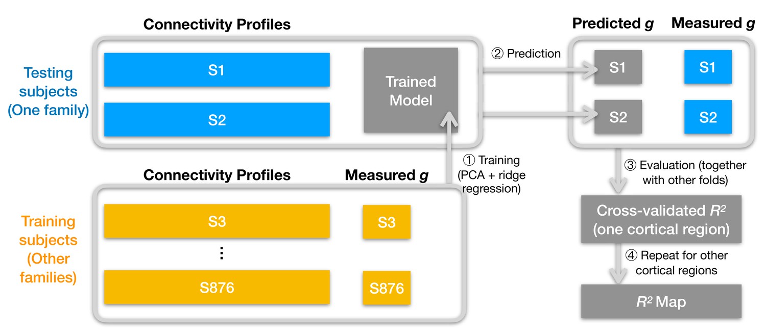
Schematic illustration of analysis pipeline.
We used a leave-one-family-out cross-validation scheme. For each data fold, we built a prediction model based on the training subjects' data (yellow color) to predict general intelligence (g) from the connectivity profile of a cortical region and applied the model to test subjects' connectivity profiles to predict their general intelligence scores (steps 1 and 2). We aggregated predicted and actually measured g across all cross-validation folds to assess model performance with cross-validated R2 (step 3) and repeated this procedure for other cortical regions' connectivity profiles (step 4). After the entire pipeline, we obtained an R2 for each of the 360 cortical regions, which stands for the amount of variance in g that can be accounted for by the region's connectivity profile. We repeated the pipeline for different kinds of connectivity profiles (spatial granularity, dataset, and alignment method) and compared them systematically (Figure 3, Figure 4, Figure 5), and these repetitions only differ in the connectivity profiles fed into the pipeline.
Figure 3
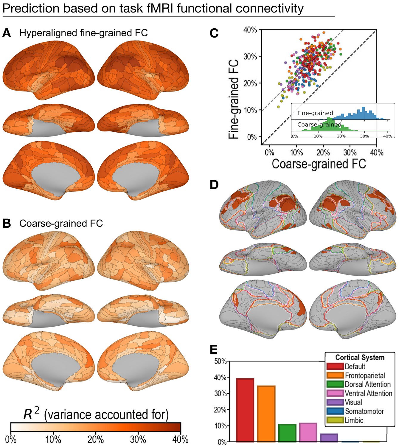
Predicting general intelligence based on regional task functional magnetic resonance imaging (fMRI) connectivity profiles.
Prediction based on hyperaligned fine-grained (A) and coarse-grained (B) connectivity profiles, assessed by the variance in general intelligence accounted for. The scatterplot (C) shows that predictions based on hyperaligned fine-grained profiles accounted for more variance in all 360 regions of interest (ROIs). Prediction models based on each region's fine-grained hyperaligned task functional connectivity profile accounted for 1.85 (95% CI: [1.70, 2.05]) times more variance in general intelligence on average than did models based on coarse-grained functional connectivity profiles. Each circle is a cortical region, and the color of each circle corresponds to the cortical system where it resides, using the same color scheme as in (E). Dashed lines denote average difference in R2 (gray) or identical R2 (black). (D) The 30 regions whose hyperaligned fine-grained connectivity best predicted general intelligence are colored as in (A) and (B). The default mode network is outlined in red, and the frontoparietal network is outlined in orange (Yeo et al., 2011). (E) Proportion of vertices in these regions that are in seven cortical systems delineated with resting state fMRI functional connectivity (Yeo et al., 2011).
Figure 4
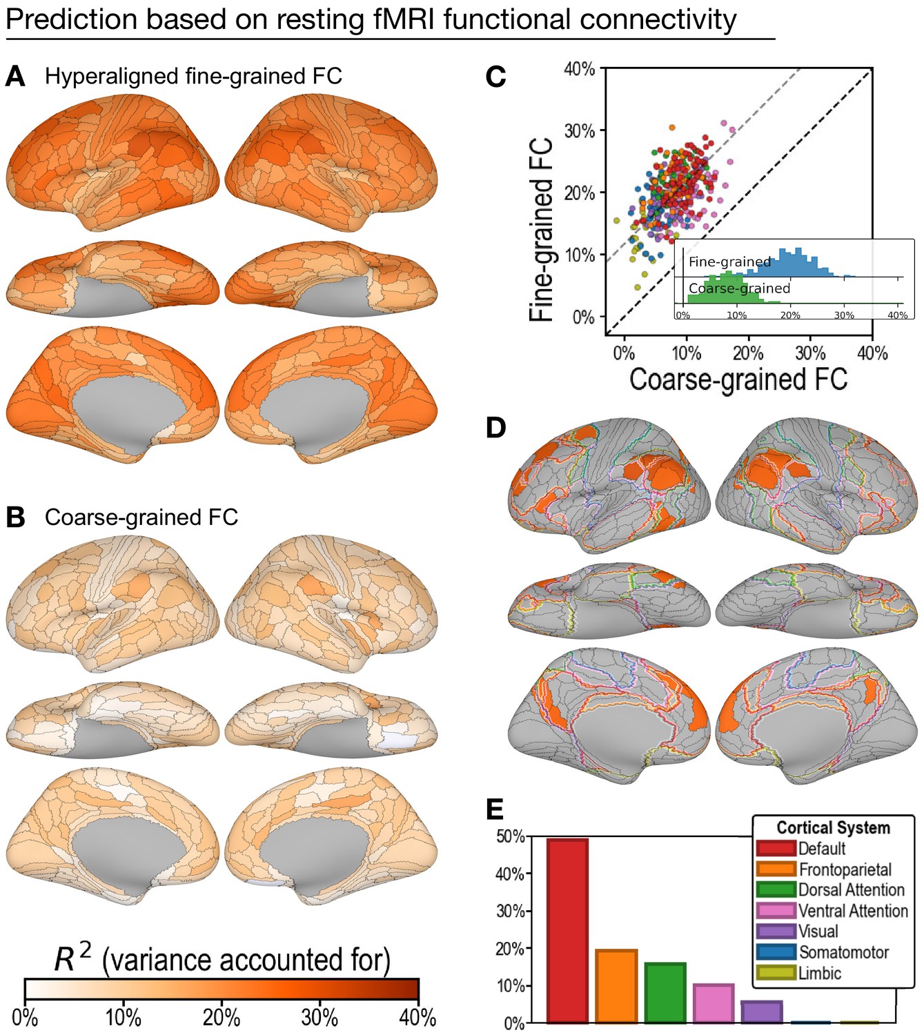
Predicting general intelligence based on regional hyperaligned resting functional magnetic resonance imaging (fMRI) connectivity profiles.
Prediction based on fine-grained (A) and coarse-grained (B) connectivity profiles. The scatterplot (C) shows that regional predictions based on hyperaligned fine-grained profiles accounted for more variance in all 360 ROIs. Prediction models based on each region's fine-grained hyperaligned resting functional connectivity profile accounted for 2.48 (95% CI: [2.18, 2.93]) times more variance in general intelligence on average than did models based on coarse-grained functional connectivity profiles. Each circle is a cortical region, and the color of each circle corresponds to the cortical system where it resides, using the same color scheme as in (E). Dashed lines denote average difference in R2 (gray) or identical R2 (black). (D) The 30 regions whose hyperaligned fine-grained connectivity best predicted general intelligence are colored as in (A) and (B). The default mode network is outlined in red, and the frontoparietal network is outlined in orange (Yeo et al., 2011). (E) Proportion of vertices in these regions that are in seven cortical systems delineated with resting state fMRI functional connectivity (Yeo et al., 2011).
Figure 5
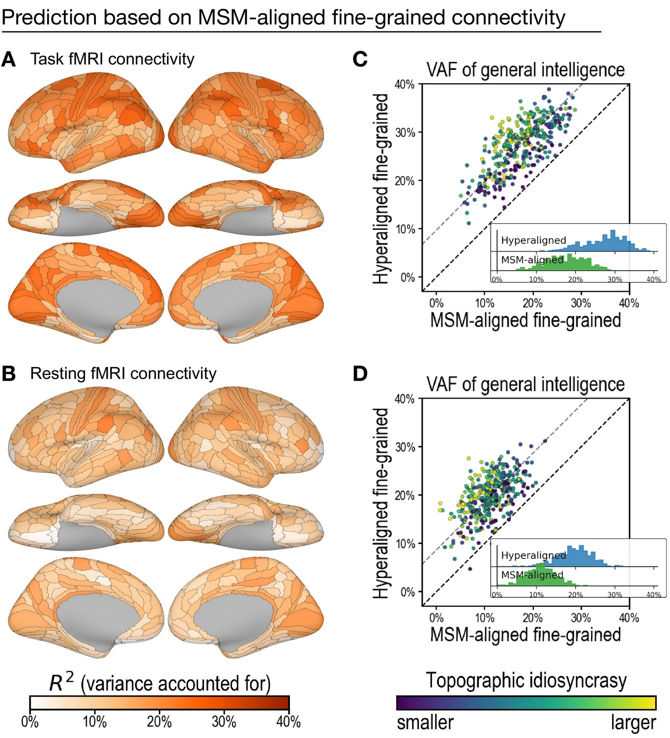
Predicting general intelligence based on multimodal surface matching (MSM)-aligned fine-grained connectivity profiles.
Prediction based on task functional magnetic resonance imaging (fMRI) (A) and resting fMRI (B) connectivity. Scatterplots compare regional predictions based on MSM-aligned to predictions based on hyperaligned task connectivity (C) and resting connectivity (D) data (comparison to results in Figure 3A , Figure 4A).
Appendix 1—figure 1
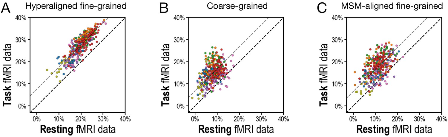
Scatterplots comparing variance accounted for by regional prediction models using task functional magnetic resonance imaging (fMRI) and resting fMRI connectivity.
(A) Hyperaligned, fine-grained connectivity. (B) Coarse-grained connectivity. (C) Multimodal surface matching-aligned fine-grained connectivity. Each circle represents one region. The color of each circle corresponds to the cortical system that each region is part of (based on a plurality of vertices), using the same color scheme as in Figure 3D and Figure 4D.
Appendix 1—figure 2
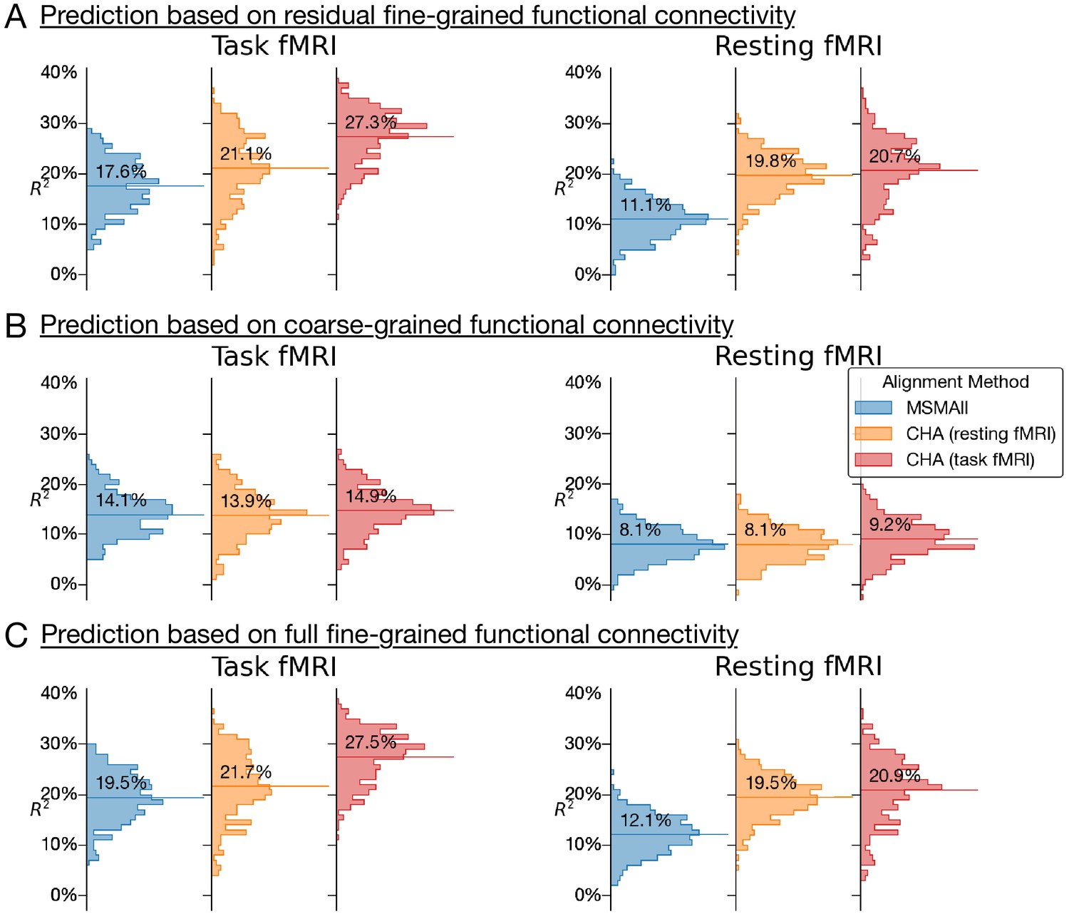
Histograms of variance accounted for by predictions of general intelligence using different functional magnetic resonance imaging connectivity datasets and different alignment methods.
(A) Prediction based on residual fine-grained connectivity. (B) Predictions based on coarse-grained connectivity. (C) Predictions based on full fine-grained connectivity, which includes information in both fine-grained and coarse-grained patterns. CHA: connectivity hyperalignment.
Appendix 1—figure 3
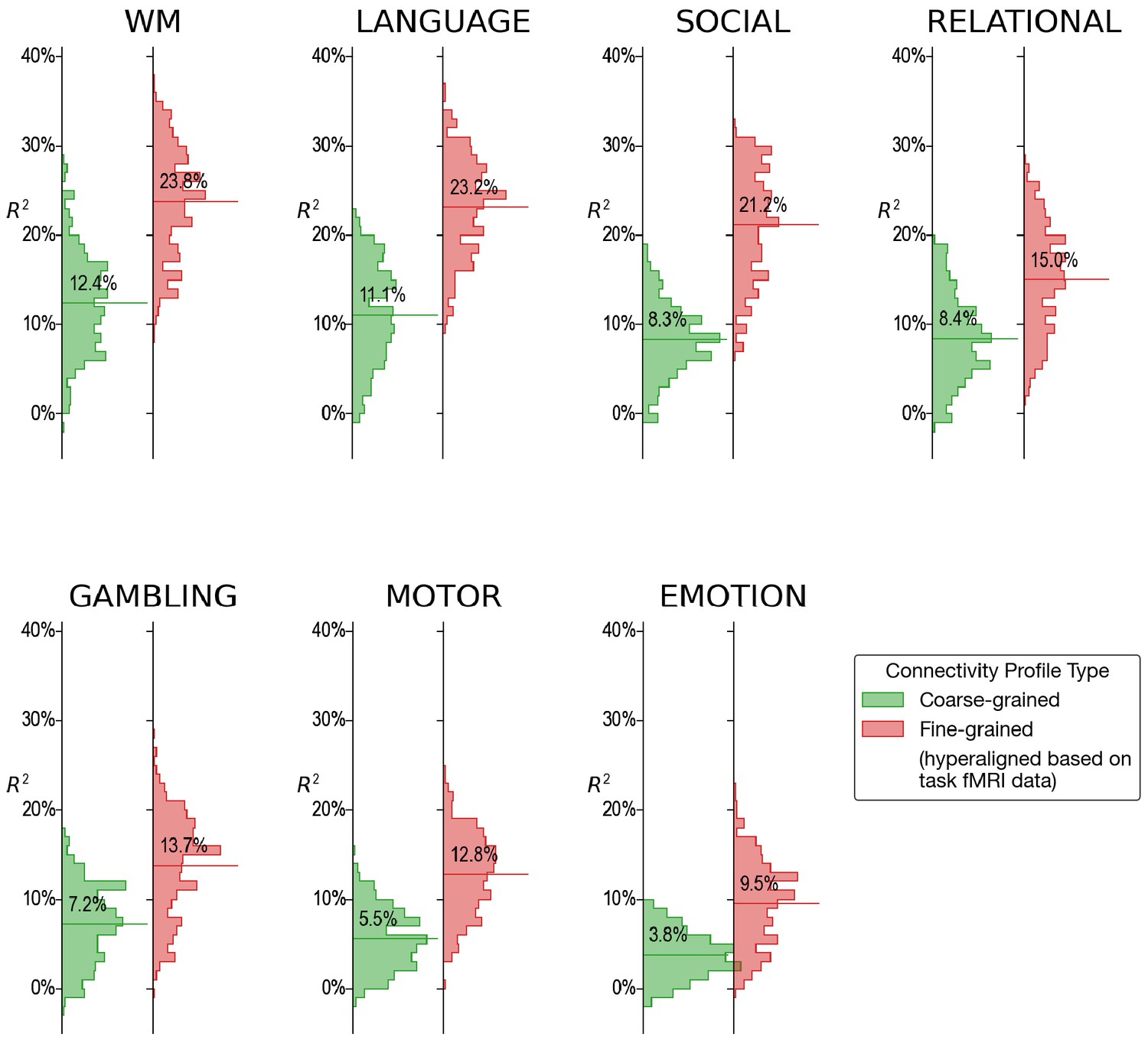
Histograms of variance accounted for by regional prediction models based on connectivity calculated from functional magnetic resonance imaging (fMRI) during single tasks.
For every single fMRI task (4.2–9.7 min), fine-scale hyperaligned connectivity data produced better predictions of general intelligence than did coarse-scale connectivity. The strongest predictions from single task fMRI were obtained from data during performance of the working memory (WM), language, and social cognition tasks.
Appendix 1—figure 4

Permutation testing. For each of the 2160 conditions (360 brain regions × 3 connectivity profile types × 2 functional magnetic resonance imaging data types), we ran a permutation test by training and evaluating prediction models 100 times based on shuffled subject labels. (A) and (B) show results based on task fMRI data and resting fMRI data, respectively.
For 2148 out of 2160 conditions (99.4%), the actual R2 was larger than all 100 permuted R2s. For the remaining 12 conditions, the actual R2 was close to 0 (all <1.3%). In other words, for any model that had an R2 of at least 1.3%, it is also larger than the maximum R2 of all 100 permutations (i.e., p < 0.01).
Appendix 1—figure 5
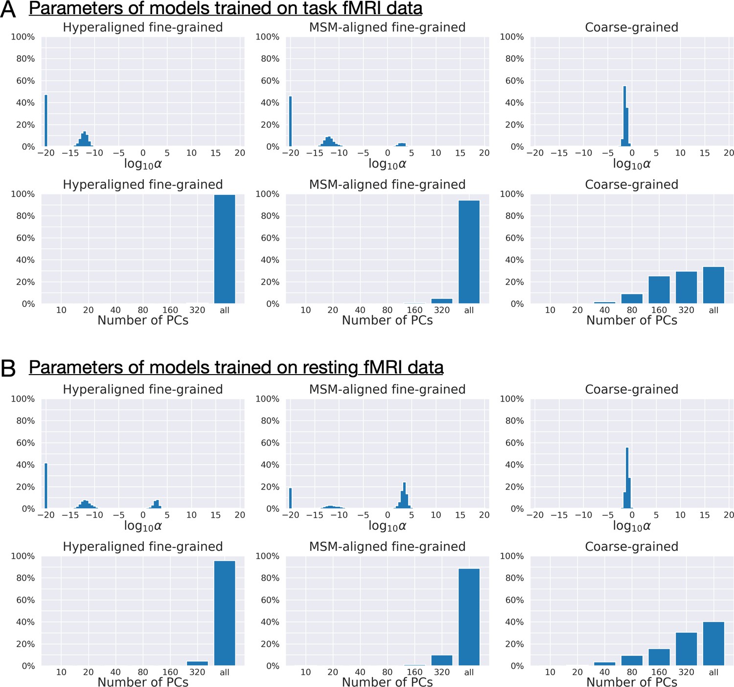
Distribution of regularization parameters α and number of principal components (PCs) for prediction models.
For each kind of functional magnetic resonance imaging (fMRI) data (A: task fMRI; B: resting fMRI) and each kind of connectivity profile (hyperaligned fine-grained, multimodal surface matching-aligned fine-grained, coarse-grained), we summarize the distribution of model parameters (the regularization parameter, α, and the number of PCs) across all cross-validation folds (411 families × 360 regions = 147,960). The maximum number of PCs was usually 360 for coarse-grained connectivity profile and close to 876 for fine-grained connectivity profile (depending on training sample size). Models trained on fine-grained connectivity profiles (left and middle columns) tend to use less regularization (smaller αs) and more PCs compared with models trained on coarse-grained connectivity profiles (right column), especially models trained on hyperaligned fine-grained connectivity profiles. More PCs used by the model suggest that there are more dimensions in the connectivity profiles that are related to general intelligence, and less regularization suggests these PCs contain more signal relative to noise.
Appendix 1—figure 6
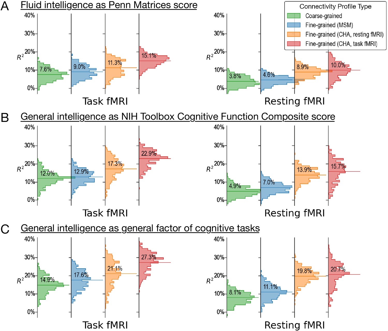
Predicting alternative measures of intelligence based on connectivity profiles.
Our prediction models and connectivity profiles can also be trained to predict other measures of intelligence, such as fluid intelligence measured with the Penn Matrices (A, variable ‘PMAT24_A_CR’ in the dataset) and general intelligence measured as the cognitive function composite score of the NIH Toolbox (B, ‘CogTotalComp_Unadj’). Similar to the results of the main paper (shown here as C for comparisons), predictions based on fine-grained hyperaligned connectivity profiles account for approximately two times more variance in intelligence compared with coarse-grained connectivity profiles for task functional magnetic resonance imaging (fMRI) data, and three times more for resting fMRI data. The four columns on the left side are based on connectivity profiles computed from task fMRI data, and the four on the right from resting fMRI data. For each kind of data, we computed fine-grained connectivity profiles based on three different alignment methods (multimodal surface matching, hyperalignment based on resting fMRI data, and hyperalignment based on task fMRI data), which we colored as blue, orange, and red, respectively. The orange and red colors denote the kind of data used to derive hyperalignment transformations. In the results shown in this figure, they may not be the same as data used to compute connectivity profiles.
Appendix 1—figure 7
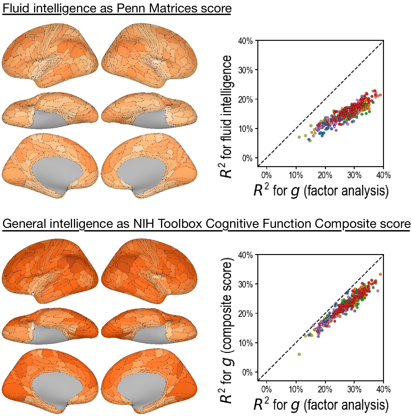
Predicting alternative intelligence measures based on regional hyperaligned fine-grained task functional magnetic resonance imaging connectivity profiles.
Regional connectivity profiles that were more predictive of factor analysis-based general intelligence scores were more likely to be more predictive of matrix reasoning-based fluid intelligence scores (top row, r = 0.92) and NIH Toolbox-based general intelligence scores (bottom row, r = 0.96). This suggests that our results were robust over intelligence measure choices.
Appendix 1—figure 8
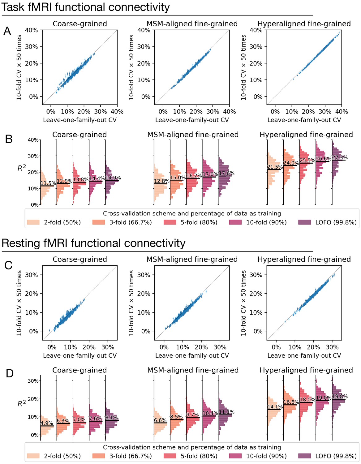
Comparison between cross-validation schemes.
We replicated our analysis using the tenfold cross-validation scheme (repeated for 50 times) and compared model performance based on tenfold cross-validation (average across 50 repetitions) with that based on leave-one-family-out cross-validation (A, C). Each dot denotes a brain region, and error bars denote the standard deviation of R2 across the 50 repetitions. All dots were close to the identity line (gray dotted line), which indicates that model performance was highly similar for leave-one-family-out cross-validation and tenfold cross-validation. On average across all regions, model performance based on leave-one-family-out cross-validation was slightly higher than that based on tenfold cross-validation, which was likely driven by the difference in training sample size (i.e., approximately 90% versus 99.8% of the entire dataset). This was confirmed by additional analysis showing further reduction of model performance based on smaller k values and correspondingly smaller training sample sizes (B, D; k = 2, 3, or 5 for k-fold cross-validation; training data was 50%, 66.7%, and 80% of the entire dataset, respectively).
Appendix 1—figure 9
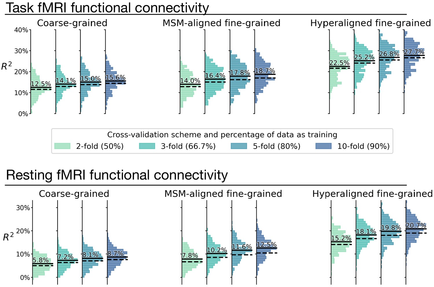
Overestimation of model performance due to lack of data independence.
We trained new prediction models based on the k-fold cross-validation scheme, but without controlling for family structure. That is, for each testing participant, other members from the same family might be in training data. Compared with the k-fold results that controlled for family structure (Appendix 1—figure 8; dashed lines in this figure), results without controlling for family structure consistently overestimate model performance (average R2 difference across regions: 0.9–2.1%; solid lines in this figure). This demonstrates the necessity of ensuring data independence between training and testing data to avoid biased model evaluations (see Varoquaux et al., 2017 for a similar issue with leave-one-trial-out). Specifically, training and testing data should not have members from the same family.
Appendix 1—figure 10

The effect of hyperparameter choices on prediction performance.
Besides using fine-tuned hyperparameters based on nested cross-validation (rightmost columns in gray), we trained prediction models based on another eight sets of hyperparameter choices. These eight sets of hyperparameters are combinations of four levels of dimensionality reduction (80 principal components [PCs], 160 PCs, 320 PCs, or all PCs) and two levels of regularization (α = 0.1 or α = 10−20). These hyperparameter levels are the levels most frequently chosen based on nested cross-validation (Appendix 1—figure 5). The histograms denote R2 distribution across brain regions, and horizontal bars are the average R2 across regions. For prediction models based on coarse-grained connectivity profiles, regularization is critical for prediction model performance, and with insufficient regularization models overfit dramatically with more PCs. When the regularization is large enough, the model performance slightly increases with higher number of PCs. For prediction models based on fine-grained connectivity profiles, model performance is hardly affected by regularization level and consistently increases with higher number of PCs. This suggests that PCs based on fine-grained connectivity profiles contain more information related to individual differences in intelligence and less noise. Note that even with only 80 PCs prediction models based on hyperaligned fine-grained connectivity profiles still account for approximately two times more variance than those based on coarse-grained connectivity profiles.
Appendix 1—figure 11
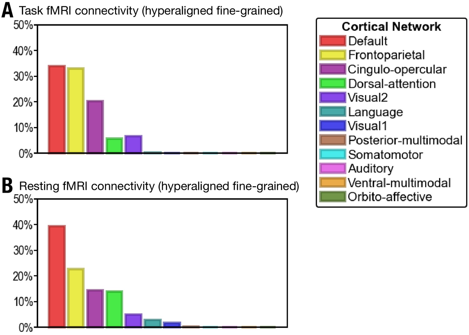
Proportion of vertices of the 30 most predictive regions in 12 cortical networks defined in Ji et al., 2019.
(A) The 30 regions that are most predictive of general intelligence based on hyperaligned fine-grained task functional magnetic resonance imaging (fMRI) connectivity are in the default (34.0% of vertices in the 30 regions), frontoparietal (33.0%), cingulo-opercular (20.2%), dorsal attention (5.7%), and visual 2 (6.7%) networks. (B) The 30 regions that are most predictive of general intelligence based on hyperaligned fine-grained resting fMRI connectivity are in the default (39.3%), frontoparietal (22.5%), cingulo-opercular (14.4%), dorsal attention (13.9%), visual 2 (4.9%), language (2.8%), and visual 1 (1.7%) networks. The 12 cortical networks are defined based on Ji et al., 2019. Note that different cortical network parcellations are in agreement with each other in general, and the proportion of cortical vertices in these 12 networks is similar to the proportion in the seven cortical systems based on Yeo et al., 2011. Most of the vertices are in default, frontoparietal, and dorsal attention networks based on both Yeo et al., 2011 and Ji et al., 2019; some regions in the ventral attention network based on Yeo et al., 2011 are labeled as cingulo-opercular in Ji et al., 2019.
Appendix 1—figure 12

Prediction performance based on a low head motion sub-sample.
General intelligence has a moderate correlation with head motion (A), and a ‘motion detector’ can predict general intelligence to some extent. To assess the effect of head motion variation on prediction performance, we trained another set of models based on a sub-sample of participants with minimal head motion (framewise displacement <0.15 mm, n = 437, B), and another 10 sets of models based on control sub-samples (see C for an example control sub-sample). The control sub-samples had similar general intelligence variation but larger head motion variation compared with the low-motion sub-sample (D). Prediction performance was similar between the low-motion sub-sample and the control sub-samples (E), suggesting larger variation in head motion level (while keeping sample size constant) has little effect on the prediction performance for general intelligence.
Appendix 1—figure 13
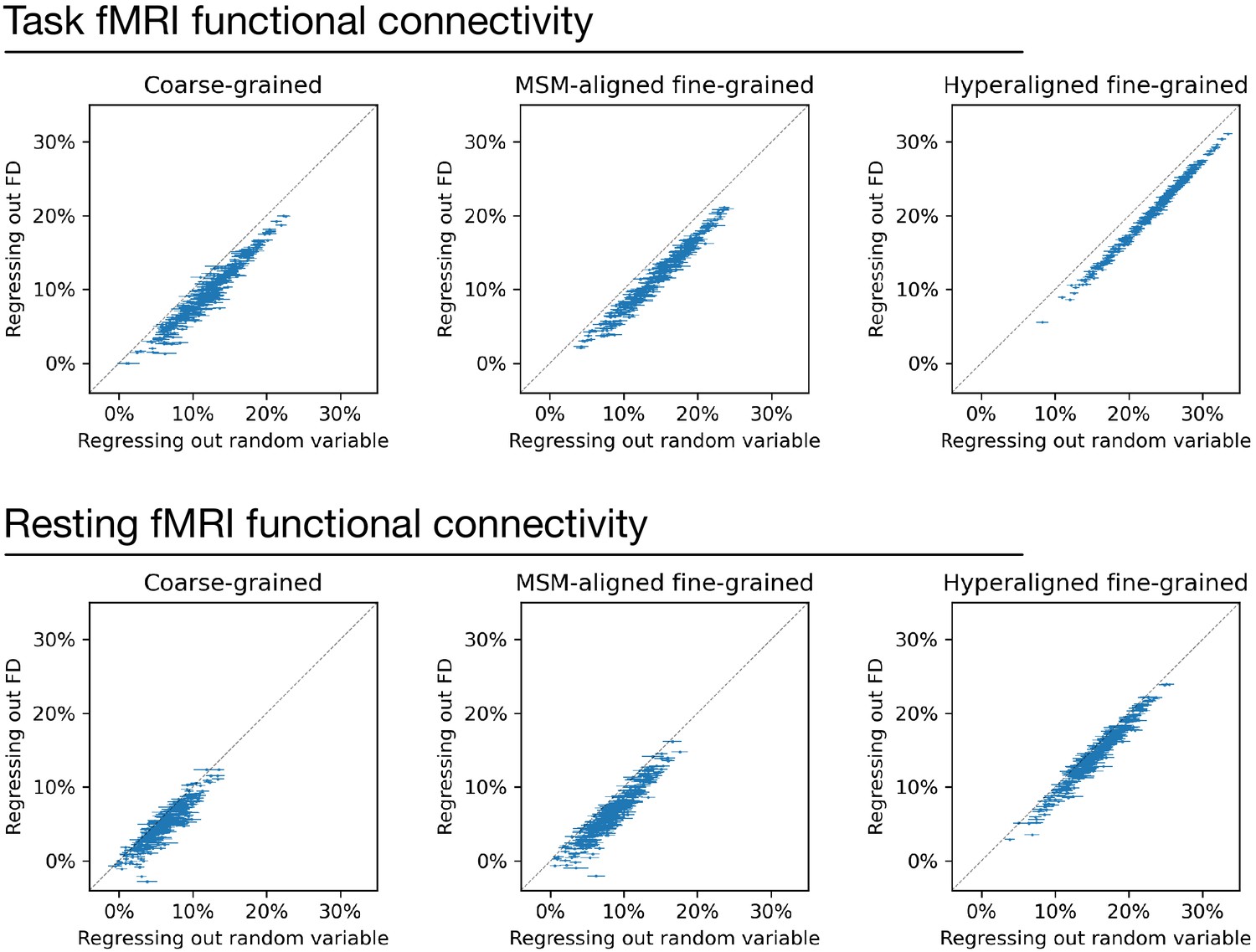
Regressing out head motion from functional connectivity.
We regressed out head motion (measured as framewise displacement) from functional connectivity profiles and built prediction models based on the residual connectivity profiles, and compared their performance with 100 sets of control models. Each dot is a brain region, and error bars denote the standard deviation across 100 control model sets. For each set of control models, a random variable that has the same level of correlation with g was regressed out from functional connectivity profiles instead of head motion to control for the effect of lower R2 ceiling caused by regression. Compared with the control models, models based on regressing out head motion had slightly lower performance (range: 1.1–2.8%), as demonstrated by that the dots are slightly below the diagonal in general. This difference suggests that the shared variance between functional connectivity and head motion may cause a slight overestimation of model performance. However, the effect is small and cannot explain the difference between models based on different types of connectivity profiles.
Additional files
Download links
A two-part list of links to download the article, or parts of the article, in various formats.
Downloads (link to download the article as PDF)
Open citations (links to open the citations from this article in various online reference manager services)
Cite this article (links to download the citations from this article in formats compatible with various reference manager tools)
The neural basis of intelligence in fine-grained cortical topographies
eLife 10:e64058.
https://doi.org/10.7554/eLife.64058


