Locus coeruleus spiking differently correlates with S1 cortex activity and pupil diameter in a tactile detection task
Figures
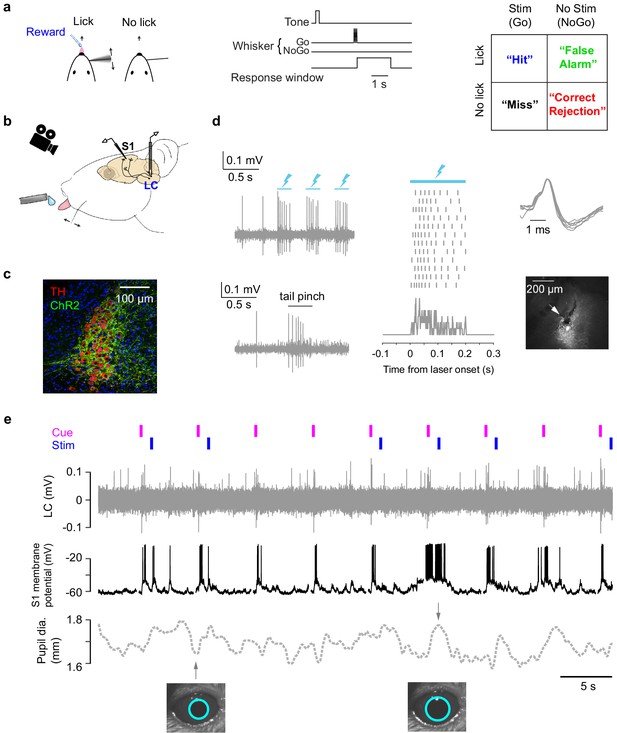
Cortical membrane potential, LC spike rate, and pupil recorded during a tactile detection task.
(a) Task schematic, trial structure, and all trial types of the single-whisker detection task (Yang et al., 2016). (b) Schematic of tetrode recording in LC, whole-cell recording in S1, and pupil tracking during the task. (c) Expression of ChR2 in a Dbh;Ai32 mouse (ChR2-EYFP: green; tyrosine hydroxylase TH: red). (d) Left: Responses of a ChR2-expressing LC unit to opto-tagging (lightning bolts: blue light pulses) and tail pinch. Middle: LC unit responses to 12 blue light pulses (200 ms) aligned to individual pulse onset. Ticks represent spikes. PSTH is shown at the bottom. Right: Typical wide waveforms of LC units and an electrolytic lesion (arrow: lesion site) in the LC (white) showing the recording location. (e) Example simultaneously recorded LC activity, S1 Vm, and pupil with auditory cue and whisker stimulation onsets indicated. Trace is from a brief period of non-performance during a behavioral session and so there are no licks. The example pupil size is typical for all sessions (Figure 1—figure supplement 1).
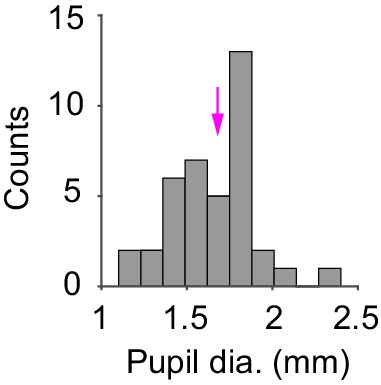
Pupil diameter across recordings.
Histogram of median pupil diameter (n = 39 recordings). Magenta arrow indicates the recording shown in Figure 1e.
-
Figure 1—figure supplement 1—source data 1
MATLAB R2016b file with median pupil diameter data.
- https://cdn.elifesciences.org/articles/64327/elife-64327-fig1-figsupp1-data1-v1.zip
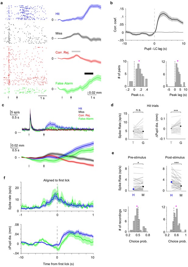
LC and pupil responses during behavior.
(a) Example LC recording with pupil tracking. Left: LC spike raster separated by trial types. Right: Mean pupil diameter (± s.e.m.) separated by trial types. Gray and black arrows indicate tone and stimulus onsets, respectively. Gray and black bars indicate the time windows during which pupil responses to tone and to Go (behavioral responses) were quantified, respectively. We note that based on the temporal profiles of pupil diameter in different trial types (i.e., in the presence or absence of tactile stimulus or licking) and that the tactile stimulus starts 1 s after tone onset, pupil responses to tone and Go can be segregated (Materials and methods). (b) Top: Grand average cross-correlogram between LC spike train and pupil diameter (n = 39). Individual LC spikes were convolved with a 400 ms wide Gaussian kernel. Spike times were shuffled and LC–pupil correlations computed to establish controls (narrow gray band around zero). Bottom: Histogram of peak correlation coefficient (left), and time lags (right) between LC spike train and pupil diameter for each paired recording (magenta dot: mean). Both distributions are significantly larger than 0 (peak correlation coefficient: 0.15 ± 0.02, p=8.3e-7, signed rank = 743; time lags: 2.61 ± 0.39 s, p=7.8e-7, signed rank = 744, n = 39). (c) Grand average trial-aligned LC spike rate (n = 43, top), and pupil diameter (n = 36, bottom) averaged by different trial types. Gray and black arrows indicate tone and stimulus onsets, respectively. In Hit trials, the latency of LC responses to tone onset was 0.064 ± 0.005 s, and to whisker stimulation onset was 0.111 ± 0.008 s, and the reaction time (first lick latency to whisker stimulation onset) of the mice was 0.58 ± 0.03 s. (d) Left: LC responses to tone (T) and Go responses (G) during Hit trials with median indicated. Tone vs. Go: 4.79 (3.70–6.66) sp/s vs. 4.68 (3.33–7.26) sp/s, median (IQR), p=0.24, signed rank = 496.5, n = 43. Right: Pupil responses to tone and Go responses during Hit trials with median indicated. Tone vs. Go: 0.003 (−0.015–0.015) mm vs. 0.027 (−0.010–0.063) mm, median (IQR), p=6.4e-5, signed rank = 559, n = 36. Gray lines indicate individual recordings. (e) Top: Pre-stimulus (baseline) and post-stimulus (evoked) LC spike rate for Hit and Miss trials with median indicated (Baseline: Hit vs. Miss, 0.66 (0.30–3.51) sp/s vs. 1.55 (0.68–3.00) sp/s, median (IQR), p=0.0083, signed rank = 254.5; Evoked: Hit vs. Miss, 3.24 (1.78–5.49) sp/s vs. 1.82 (0.95–3.45) sp/s, median (IQR), p=5.5e-7, signed rank = 782.5, n = 43). Gray lines indicate individual recordings. Bottom: Histogram of choice probability for Hit vs. Miss trials based on baseline and evoked LC activity (magenta dots: mean). Choice probabilities are significantly deviated from 0.5. Baseline: 0.47 ± 0.014, p=0.032, signed rank = 295.5; Evoked: 0.59 ± 0.017, p=4.6e-6, signed rank = 751, n = 43. (f) Lick-aligned LC spike rate (top) and pupil diameter (∆Pupil, bottom) averaged by trial types: Hit (blue), FA (green).
-
Figure 2—source data 1
MATLAB R2016b file with data shown in panels b, d and e.
- https://cdn.elifesciences.org/articles/64327/elife-64327-fig2-data1-v1.zip
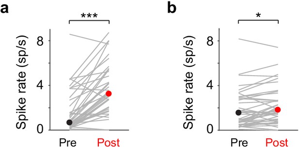
LC responses during Hit and Miss trials.
(a) Hit trials: Pre-stimulus vs. post-stimulus: 0.66 (0.30-3.51) sp/s vs. 3.24 (1.78-5.49) sp/s, median (IQR), P = 7.6e-7, n = 43. (b) Miss trials: Pre-stimulus vs. post-stimulus: 1.55 (0.68-3.00) sp/s vs. 1.82 (0.95-3.45) sp/s, median (IQR), P = 0.02, n = 43.
-
Figure 2—figure supplement 1—source data 1
MATLAB R2016b file with data shown in panels a and b.
- https://cdn.elifesciences.org/articles/64327/elife-64327-fig2-figsupp1-data1-v1.zip
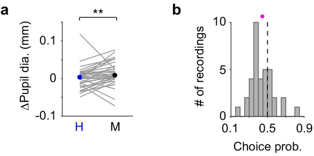
Pupil responses to the tone during Hit and Miss trials.
(a) Pupil responses to the tone for Hit and Miss trials with median indicated. Hit vs. Miss, 0.003 (-0.015 – 0.015) mm vs. 0.0083 (-0.0005 – 0.029) mm, median (IQR), P = 0.0062, n = 36. Gray lines indicate individual recordings. (b) Histogram of choice probability for Hit vs. Miss trials based on pupil responses to the tone (magenta dot: mean). Choice probability is significantly deviated from 0.5 (0.44 ± 0.021, P = 0.0036, n = 36).
-
Figure 2—figure supplement 2—source data 1
MATLAB R2016b file with pupil and choice probability data shown in panels a and b.
- https://cdn.elifesciences.org/articles/64327/elife-64327-fig2-figsupp2-data1-v1.zip
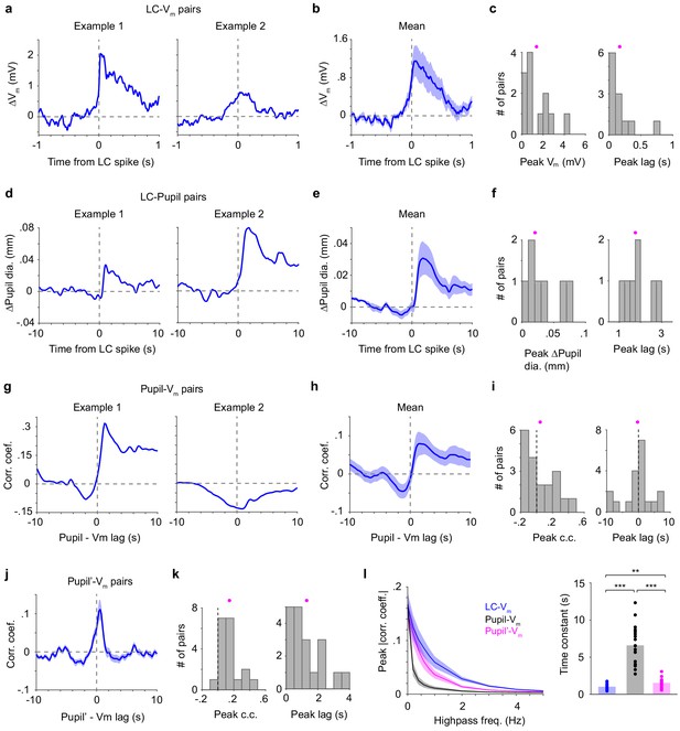
Different relationships between LC spikes, S1 Vm, and pupil diameter.
(a) Two examples of LC spike-triggered average ∆Vm. (b) Group mean of LC spike-triggered average ∆Vm (± s.e.m., n = 12). (c) Histograms of peak ∆Vm and peak lags (showing all LC–S1 pairs) with means indicated (magenta dots). Both distributions are significantly larger than 0 (peak ∆Vm: 1.39 ± 0.35 mV, p=4.9e-4, signed rank = 78; peak lags: 0.17 ± 0.06 s, p=4.9e-4, signed rank = 78, n = 12). (d) Two examples of LC spike-triggered average ∆Pupil. (e) LC spike-triggered average ∆Pupil group mean (± s.e.m., n = 7). (f) Histograms of peak ∆Pupil and peak lags (showing all LC–Pupil pairs) with means indicated (magenta dots). Both distributions are significantly larger than 0 (peak ∆Pupil: 0.03 ± 0.01 mm, p=0.016, signed rank = 28; peak lags: 1.89 ± 0.25 s, p=0.016, signed rank = 28, n = 7). (g) Two examples of Pupil–Vm cross-correlograms. (h) Group mean of Pupil–Vm cross-correlograms (± s.e.m., n = 19). (i) Histograms of peak Pupil–Vm correlation coefficient and peak lags (showing all S1–Pupil pairs) with means indicated (magenta dots). Both distributions are not significantly deviated from 0 (peak correlation coefficient: 0.05 ± 0.04, p=0.33, signed rank = 119; peak lags: - 0.22 ± 1.01 s, p=0.87, signed rank = 99, n = 19). (j) Group mean of the time derivative of pupil (Pupil’)–Vm cross-correlograms (± s.e.m., n = 19). (k) Histograms of peak Pupil’-Vm correlation coefficient and peak lags with means indicated (magenta dots). Both distributions are significantly larger than 0 (peak correlation coefficient: 0.15 ± 0.03, p=1.6e-4, signed rank = 189; peak lags: 1.31 ± 0.24 s, p=1.3e-4, signed rank = 190, n = 19). (l) Left: Peak correlation coefficient for LC–Vm, Pupil–Vm and Pupil’–Vm pairs after progressive high-pass filtering of S1 Vm. Right: Exponential decay functions (corr. coef. = a*exp(−freq*μ)) were fitted to these curves. The time constant μ is significantly different (repeated-measures ANOVA, F(2, 36)=74.5, p=1.6e-13, n = 19). Post hoc Tukey–Kramer tests revealed that the LC–Vm relationship had the slowest decay and Pupil–Vm had the fastest decay. LC–Vm vs. Pupil–Vm, p=5.9e-8; LC–Vm vs. Pupil’–Vm, p=0.0037; Pupil–Vm vs. Pupil’–Vm, p=7.1e-7.
-
Figure 3—source data 1
MATLAB R2016b file with data shown in Figure 3 c, f, i, k and l.
- https://cdn.elifesciences.org/articles/64327/elife-64327-fig3-data1-v1.zip
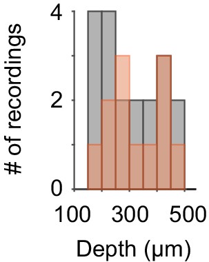
Histograms of the depth of S1 whole-cell recordings.
Red: 12 S1 recordings included in the LC–S1 pairs in Figures 3a–c and 4a. Gray: 19 S1 recordings included in the Pupil–S1 pairs in Figure 3g–I.
-
Figure 3—figure supplement 1—source data 1
MATLAB R2016b file with recording depth data.
- https://cdn.elifesciences.org/articles/64327/elife-64327-fig3-figsupp1-data1-v1.zip
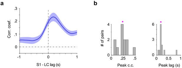
Cross-correlation between LC spikes and S1 Vm.
(a) Group mean of cross-correlogram between LC spike train and S1 Vm (n = 12). Individual LC spikes were convolved with a 400 ms wide Gaussian kernel. (b) Histogram of peak correlation coefficient (0.24 ± 0.03) and time lag (0.24 ± 0.06 s) between LC spike train and S1 Vm for each paired recording (magenta dot: mean).
-
Figure 3—figure supplement 2—source data 1
MATLAB R2016b file with data shown in panel b.
- https://cdn.elifesciences.org/articles/64327/elife-64327-fig3-figsupp2-data1-v1.zip
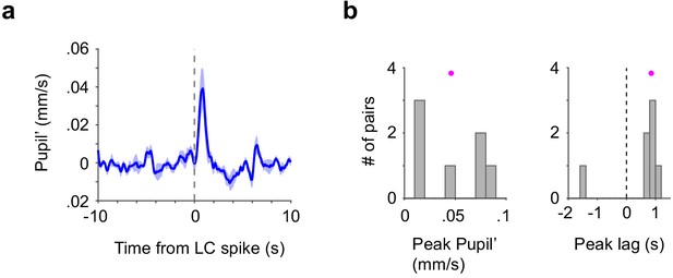
LC spike-triggered time derivative of pupil diameter.
(a) Group mean of LC spike-triggered time derivative of pupil diameter (Pupil’, n = 7), same dataset as used in Figure 3d–f. (b) Histogram of peak pupil’ (0.05 ± 0.01 mm/s) and time lag (0.53 ± 0.35 s) between LC spike train and pupil’ for each paired recording (pupil dot: mean).
-
Figure 3—figure supplement 3—source data 1
MATLAB R2016b file with data shown in panel b.
- https://cdn.elifesciences.org/articles/64327/elife-64327-fig3-figsupp3-data1-v1.zip
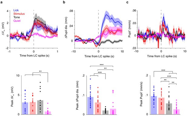
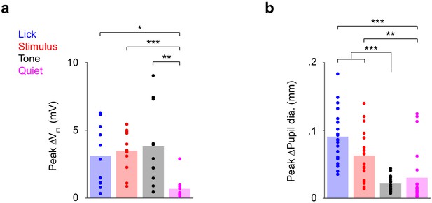
Correlations between LC spikes, S1 Vm, and pupil diameter depend on task epoch.
(a) Top: LC spike-triggered ∆Vm separated by task epoch: tone, stimulus, lick, and quiet. Bottom: Bar graphs of peak ∆Vm for each epoch. Dots indicate individual paired recordings. Repeated-measure ANOVA, F(3, 33)=9.2, p=1.4e-4, n = 12. Post hoc Tukey–Kramer tests revealed that peak ∆Vm in lick, stimulus, and tone epochs were not different from each other. Lick vs. Stim, p=1.00; Lick vs. Tone, p=0.76; Stim vs. Tone, p=0.94. Peak ∆Vm in quiet epochs was lower. Quiet vs. Lick, p=0.0059; Quiet vs. Stim, p=0.0038; Quiet vs. Tone, p=0.0041. (b) Top: LC spike-triggered ∆Pupil separated by task epoch. Bottom: Bar graphs of peak ∆Pupil for each epoch. Dots indicate individual paired recordings. Repeated-measure ANOVA, F(3, 57)=22.1, p=1.3e-9, n = 20. Post hoc Tukey–Kramer tests revealed that peak ∆Pupil in lick and stimulus epochs were larger than in tone and quiet epochs. Lick vs. Stim, p=0.10; Tone vs. Quiet, p=0.76; Lick vs. Tone, p=3.7e-7; Lick vs. Quiet, p=6.2e-4; Stim vs. Tone, p=1.1e-4; Stim vs. Quiet, p=0.0027. (c) Top: LC spike-triggered pupil’ separated by task epoch. Bottom: Bar graphs of peak pupil’ for each epoch. Dots indicate individual paired recordings. Repeated-measures ANOVA, F(3, 57)=35.3, p=4.9e-13, n = 20. Post hoc Tukey–Kramer tests revealed that peak pupil’ in lick and stimulus epochs were larger than in tone, and peak pupil’ in quiet epochs was the lowest. Lick vs. Stim, p=0.46; Tone vs. Quiet, p=0.0013; Lick vs. Tone, p=1.0e-4; Lick vs. Quiet, p=1.4e-8; Stim vs. Tone, p=0.0058; Stim vs. Quiet, p=6.7e-6.
-
Figure 4—source data 1
MATLAB R2016b file with data shown in Figure 4a–c.
- https://cdn.elifesciences.org/articles/64327/elife-64327-fig4-data1-v1.zip
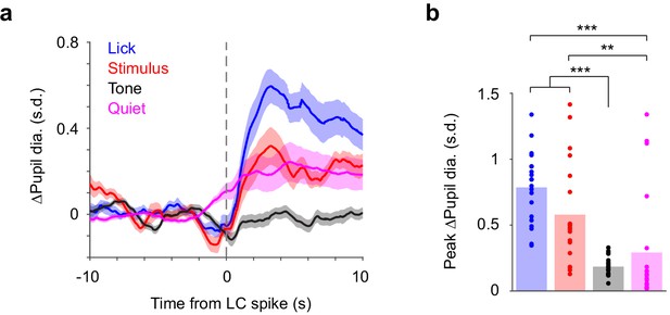
Correlations between LC spikes and z-scored pupil diameter depend on task epoch.
(a) LC spike-triggered z-scored ∆Pupil separated by task epoch. (b) Bar graphs of z-scored peak ∆Pupil for each epoch. Dots indicate individual paired recordings. Repeated-measure ANOVA, F(3, 57)=21.4, p=2.1e-9, n = 20. Post hoc Tukey–Kramer tests revealed that z-scored peak ∆Pupil in lick and stimulus epochs were larger than in tone and quiet epochs. Lick vs. Stim, p=0.16; Tone vs. Quiet, p=0.65; Lick vs. Tone, p=3.0e-8; Lick vs. Quiet, p=3.3e-4; Stim vs. Tone, p=3.0e-4; Stim vs. Quiet, p=0.0087.
-
Figure 4—figure supplement 1—source data 1
MATLAB R2016b file with data shown in panel b .
- https://cdn.elifesciences.org/articles/64327/elife-64327-fig4-figsupp1-data1-v1.zip
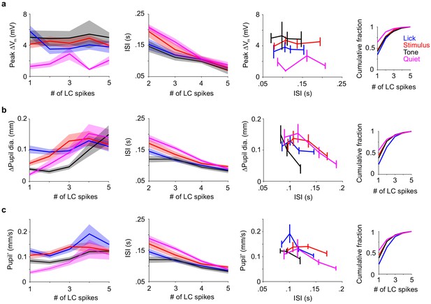
Dependencies of pupil diameter, pupil' and Vm depolarization on LC spike count.
(a) From left to right: (1) Peak ∆Vm vs. LC spike counts by epoch. (2) Inter-spike-interval vs. LC spike counts by epoch. Quiet and Stimulus epochs differ for the Vm response across LC spike counts, but their ISIs are similar. At low spike counts, Quiet and Tone epochs differ for both Vm response and ISI. ∆Vm for LC spike counts 2-5, Quiet vs. Stim: P = 9.9e-4, 0.081, 0.016, 0.14; Quiet vs. Tone: P = 0.0043, 0.062, 0.11, 0.19. ISI for LC spike counts 2-5, Quiet vs. Stim: P = 0.44, 0.25, 1, 0.79; Quiet vs. Tone: P = 0.0061, 0.0068, 0.20, 0.38. Two-tailed Wilcoxon rank sum test. (3) Peak ∆Vm vs. mean inter-spike-interval for LC spike counts 2-5. This is essentially replotting the values in the y axis in (1) against the values in y axis in (2). (4) Cumulative histograms showing numbers of trials that go into the plots when broken down by LC spike counts. (b) From left to right: (1) Peak ∆Pupil vs. LC spike counts by epochs. (2) Inter-spike-interval vs. LC spike counts by epochs. (3) Peak ∆Pupil vs. mean inter-spike-interval for LC spike counts 2-5. (4) Cumulative histograms showing numbers of trials that go into the plots when broken down by LC spike counts. (c) From left to right: (1) Peak Pupil’ vs. LC spike counts by epochs. (2) Inter-spike-interval vs. LC spike counts by epochs, identical to what is shown in b. (3) Peak Pupil’ vs. mean inter-spike-interval for LC spike counts 2-5. (4) Cumulative histograms showing numbers of trials that go into the plots when broken down by LC spike counts, which is identical to the histogram in (b).
Analysis using an alternative window to define the ‘Tone’ epoch.
Bar graphs of peak ∆Vm (a) and ∆Pupil (b) for each epoch, when ‘Tone’ epochs were defined 0 s to 0.5 s with respect to tone onset.
-
Figure 4—figure supplement 3—source data 1
MATLAB R2016b file with data shown in panels a,b.
- https://cdn.elifesciences.org/articles/64327/elife-64327-fig4-figsupp3-data1-v1.zip
Tables
| Reagent type (species) or resource | Designation | Source or reference | Identifiers | Additional information |
|---|---|---|---|---|
| Strain, strain background (M. musculus) | DBH-Cre | MMRRC | Cat# 036778-UCD, RRID:MMRRC_036778-UCD | |
| Strain, strain background (M. musculus) | Ai32 | Jackson Laboratory | Cat#: JAX:012569, RRID:IMSR_JAX:012569 | |
| Software, algorithm | BControl | Princeton University | https://brodylabwiki.princeton.edu/bcontrol | |
| Software, algorithm | WaveSurfer | HHMI Janelia | http://wavesurfer.janelia.org/ | |
| Software, algorithm | MATLAB | MathWorks | RRID:SCR_001622 | |
| Software, algorithm | StreamPix | Norpix | RRID:SCR_015773 | |
| Software, algorithm | Adobe Illustrator | Adobe | RRID:SCR_010279 | |
| Other | High-speed CMOS camera | PhotonFocus | DR1-D1312-200-G2-8 | |
| Other | Telecentric lens | Edmund Optics | Cat#: 55–349 | |
| Other | Pipette glass | Warner Instruments | Cat#: 640792 | |
| Other | Tetrode drive | Cohen et al., 2012 | N/A | |
| Antibody | Anti-TH primary antibody (rabbit, polyclonal) | Thermo-Fisher | Cat#: OPA1-04050, RRID: AB_325653 | (1:1000) |
| Antibody | Secondary antibody (goat, polyclonal) | Thermo-Fisher | Cat#: A-11008, RRID:AB_2534079 | (1:500) |


