Hippocampal replay of experience at real-world speeds
- Howard Hughes Medical Institute, University of California, San Francisco, United States
- Departments of Physiology and Psychiatry, University of California, San Francisco, United States
- Kavli Institute for Fundamental Neuroscience, University of California, San Francisco, United States
- Department of Neurobiology, Stanford University School of Medicine, United States
- Department of Neurological Surgery, University of California, San Francisco, United States
- Department of Mathematics and Statistics, Boston University, United States
Figures
Figure 1 with 1 supplement

The model can capture different sequence dynamics on simulated data.
(A) We construct a firing sequence of 19 simulated place cells that exhibits three different movement dynamics. For the first 60 ms, one cell fires repeatedly, representing one stationary location. For next 190 ms, the cells fire in sequence, representing a rapid continuous trajectory along the virtual track. For the last 30 ms, cells fire randomly, out of spatial order, representing an fragmented spatial sequence. (B) Like the standard decoder, the state space model uses estimates of cells’ place fields from when the animal is moving and combines them with the observed spikes in (A) to compute the likelihood of position for each time step. (C) The prediction from the neural data is then combined with an explicit model of each movement dynamic, which determines how latent position can change based on the position in the previous time step. We show the probability of the next position bin for each movement dynamic model (color scale). Zero here represents the previous position. (D) The probability of remaining in a particular movement dynamic versus switching to another dynamic is modeled as having a high probability of remaining in a particular dynamic with a small probability of switching to one of the other dynamics at each time step. (E) The model uses the components in A-D over all time to decode the joint posterior probability of latent position and dynamic. This can be summarized by marginalizing over latent position (left panel) to get the probability of each dynamic over time. The shaded colors indicate the category of the speed of the trajectory at that time (Stat. = Stationary, S-C-M = Stationary-Continuous-Mixture, Cont. = Continuous, F-C-M = Fragmented-Continuous-Mixture, Frag. = Fragmented), which is determined from the probability. Marginalizing the posterior across dynamics also provides an estimate of latent position over time (right panel). Red dotted line in the right panel is the best fit line from the standard decoder using the Radon transform. (F) The probability of each dynamic depends heavily on the speed of the trajectory, as we show using a range of simulated spiking sequences each moving at a constant speed. Each dot corresponds to the average probability of that dynamic for a given constant speed sequence. We use a 0.80 threshold (dotted line) to classify each sequence based on the dynamic or dynamics which contribute maximally to the posterior (shaded colors).
Figure 1—figure supplement 1
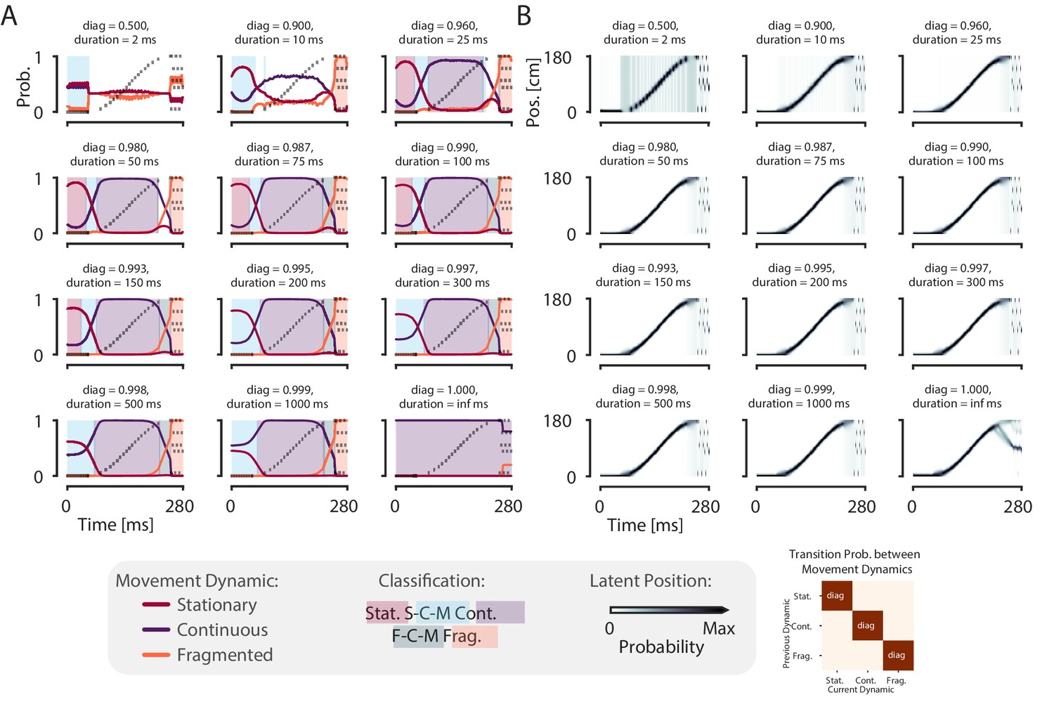
The model is robust to change of the probability of persisting in the same dynamic for a wide range of plausible expected durations (25–150 ms).
(A) Each panel shows the probability of each dynamic on simulated data example from Figure 1 with a different diagonal value—which governs the probability of remaining in that dynamic. The corresponding expected duration of staying in the dynamic is listed as duration. The off-diagonal values—the probability of switching to one of the other dynamics—are set to be equally likely with the remainder of the probability, as in Figure 1D. The diagonal increases from left to right, top to bottom, until the case where the diagonal is one and the off-diagonal is zero—that is the case where there is no probability of switching to another dynamic. Shaded regions correspond to the classification as in Figure 1F. (B) The probability of position over time for each diagonal value. Conventions the same as in (A).
Figure 2 with 4 supplements
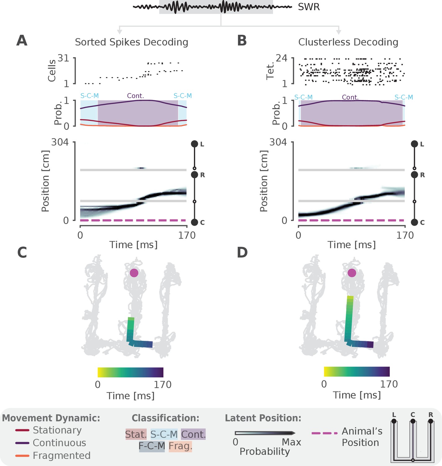
The model can decode hippocampal replay trajectories using either sorted and clusterless spikes from the same SWR event.
(A) Decoding using sorted spikes. The top panel shows 31 cells on a W-track ordered according to linearized position by their place field peaks. The middle panel shows the probability of each dynamic over time as in Figure 1E, left panel. Shaded regions correspond to the speed classifications as in Figure 1F. The bottom panel shows the estimated probability of latent position over the course of the SWR as it travels down the center arm toward the right arm. L, R, C correspond to the position of the left, right and center reward wells, respectively. The animal’s actual position is indicated by the the magenta dashed line. Underneath is the maximum of the 1D decoded position (the most probable position) projected back onto the 2D track for the sorted decoding. Color indicates time. The animal’s actual position is denoted by the pink dot. Light gray lines show the animal’s 2D position over the entire recording session. (B) Decoding using clusterless spikes. The top panel shows multiunit spiking activity from each tetrode. Other panels have the same convention as (A). Underneath is the maximum of the 1D decoded position (the most probable position) projected back into 2D using the clusterless decoding.
Figure 2—figure supplement 1
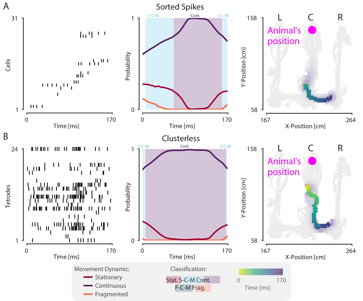
Decoding the same SWR in Figure 2 with 2D position using sorted spikes and clusterless decoding.
(A) The left panel shows the spikes from cells arranged by the linear position of the peak of place field as in Figure 2. The middle panel shows the probability of each dynamic over time from the 2D decode. Shaded regions indicate classification category as in Figure 1F and Figure 2. The rightmost panel shows the most probable estimate of the latent position (MAP estimate) with color indicating time. The latent position posterior summed over time is shown in the purple shading. The light gray lines represent the position of the animal over the entire recording session and the magenta dot represents the animal’s position. (B) Same as in (A), but with clusterless decoding.
Figure 2—figure supplement 2
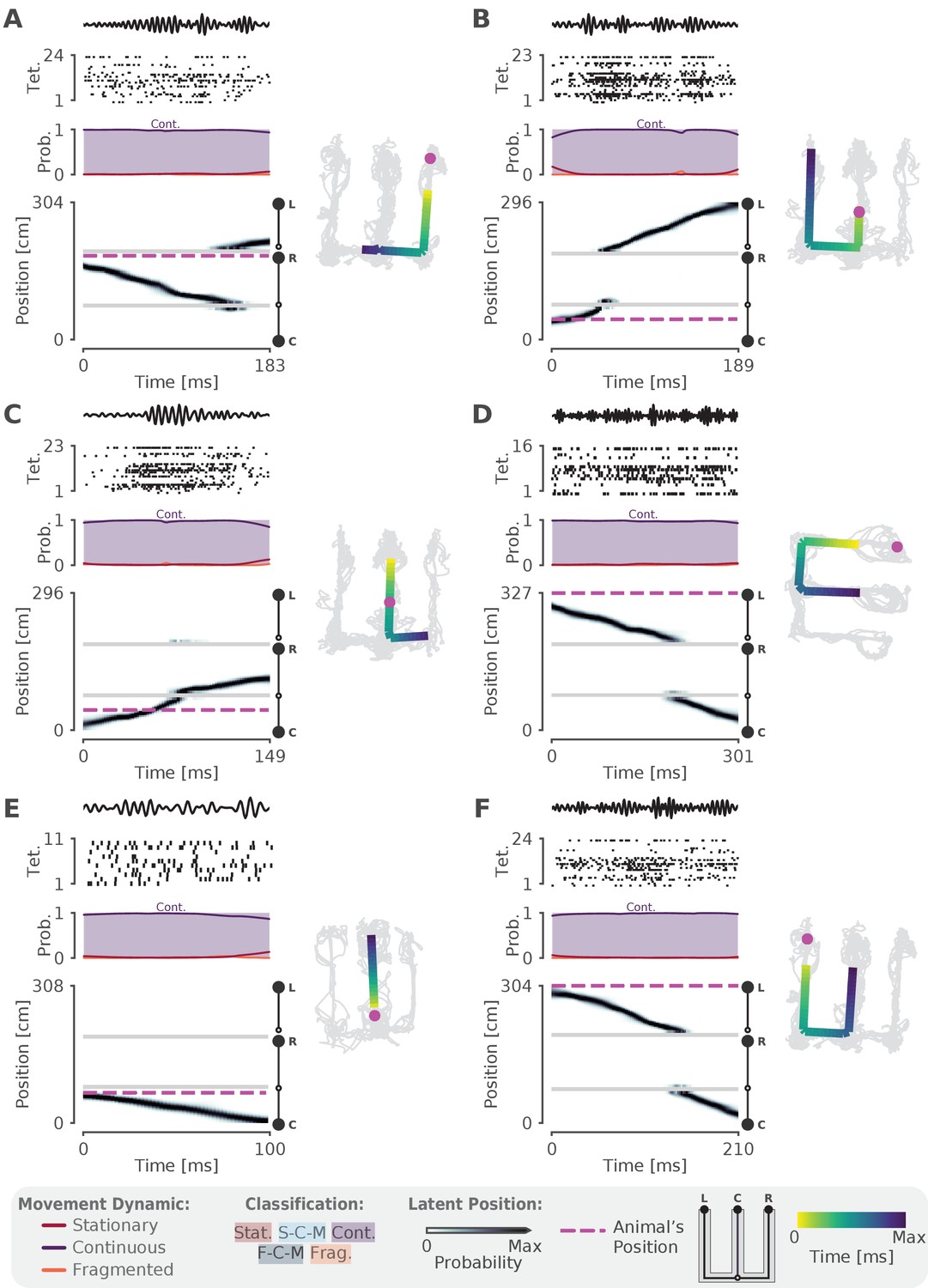
More examples of SWRs that have continuous trajectories.
(A-F) More examples of SWRs that have continuous trajectories. Left panel uses the same conventions as Figure 2A and Figure 2B. Right panel shows the 1D MAP estimate projected back to 2D as in Figure 2C. Color indicates time. Light gray lines indicate the animal’s position over the entire recording session. Magenta dashed line represents the animal’s position during the SWR.
Figure 2—figure supplement 3
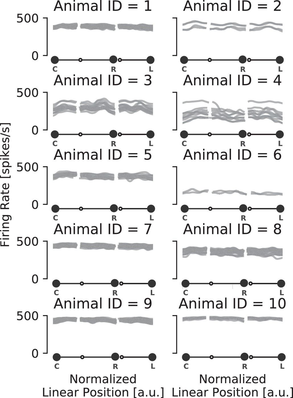
Population firing rate on the track is spatially uniform and consistent for each animal.
Multiunit rate of encoding spikes over track positions for each animal. Each gray line represents a recording session for that animal.
Figure 2—video 1
Example of an SWR with continuous content.
Magenta dot represents the animal’s position. Green dot represents the most likely decoded position projected from 1D back to the linearized 2D position. Green line represents the decoded positions in the last 10 ms. Gray lines represent the position of the animal over the course of the recording session.
Figure 3 with 4 supplements
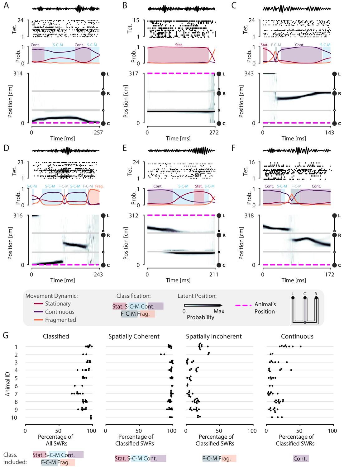
Most SWRs are spatially coherent, but not continuous.
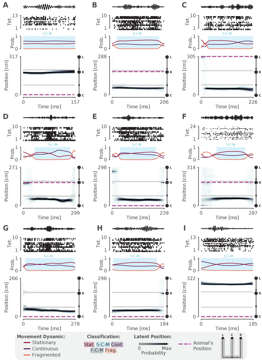
(A-F) Examples of SWRs with non-constant speed trajectories. Figure conventions are the same as in Figure 2. Filtered SWR ripple (150–250 Hz) trace from the tetrode with the maximum amplitude displayed above each example. (A) An SWR where the decoded position starts moving down the center arm away from the animal’s position at the center well, slows down, and returns back. (B) An SWR where the decoded position persistently stays at the choice point (open circle) while the animal remains at the left well. (C) An SWR where the decoded position begins with stationary representation of the left well, then jumps to the middle of the right arm and proceeds up the right arm to the right well. (D) An SWR where the decoded position begins with stationary representation of the left well, jumps to the center arm, proceeds away from the center well, jumps to the right arm, proceeds back toward the center well, and then becomes fragmented. (E) An SWR where the decoded position begins in the left arm and persists at the end of the center arm. (F) An SWR where the decoded position starts in the left arm toward the choice point, jumps to the right arm and proceeds back toward the choice point. (G) Classification of SWRs from multiple animals and datasets. Each dot represents the percentage of SWRs for each day for that animal. An SWR is included in the numerator of the percentage if at any time it includes the classifications listed below the column. The denominator is listed in the x-axis label.
-
Figure 3—source data 1
Table of replay statistics for each SWR for Figure 3G.
- https://cdn.elifesciences.org/articles/64505/elife-64505-fig3-data1-v2.csv
Figure 3—figure supplement 1
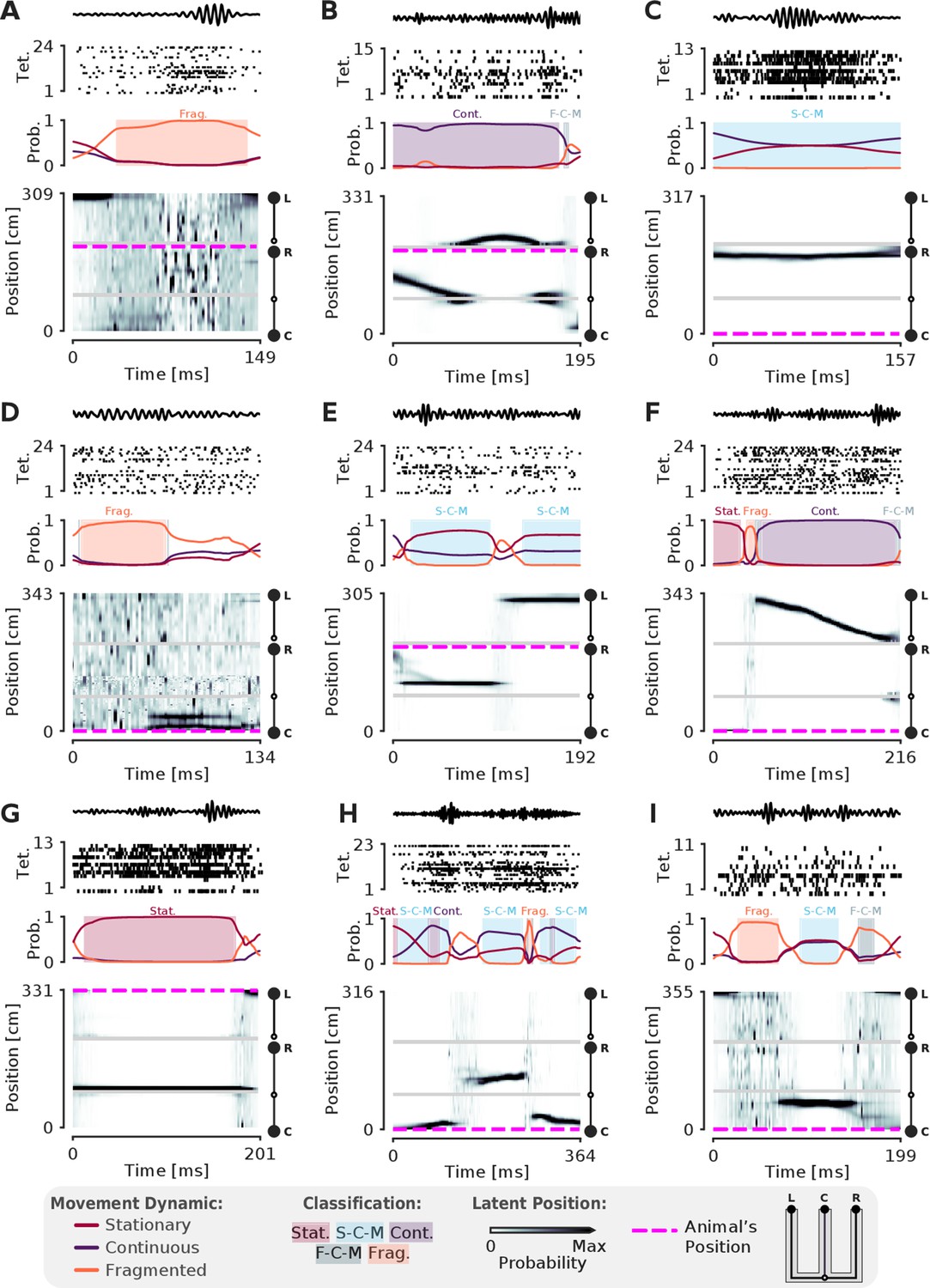
More examples of SWRs with non-constant speed trajectories.
(A-I) More examples of SWRs with non-constant speed trajectories. Conventions are the same as in Figure 3.
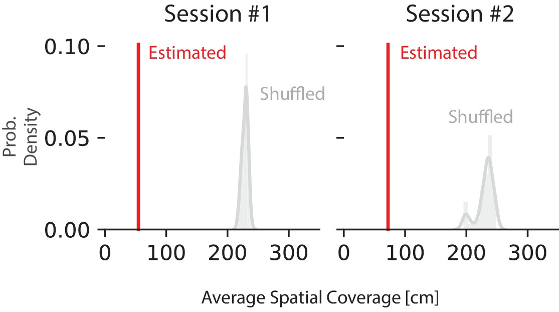
Figure 3—figure supplement 2
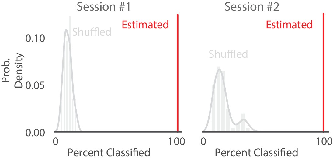
Shuffling the position data with replacement decreases the percent of SWRs classified.
Comparison of percentage of SWRs classified (that is, an SWR containing at least one of the five classifications) on real vs. position shuffled data for two recording sessions from different animals. Red line represents the percent of SWR events classified in that recording session for real data. The histogram represents the distribution after 50 shuffles of the position data. Position data was shuffled by resampling with replacement from the set of all observed positions in that recording session, destroying position information but preserving spiking timing and position occupancy.
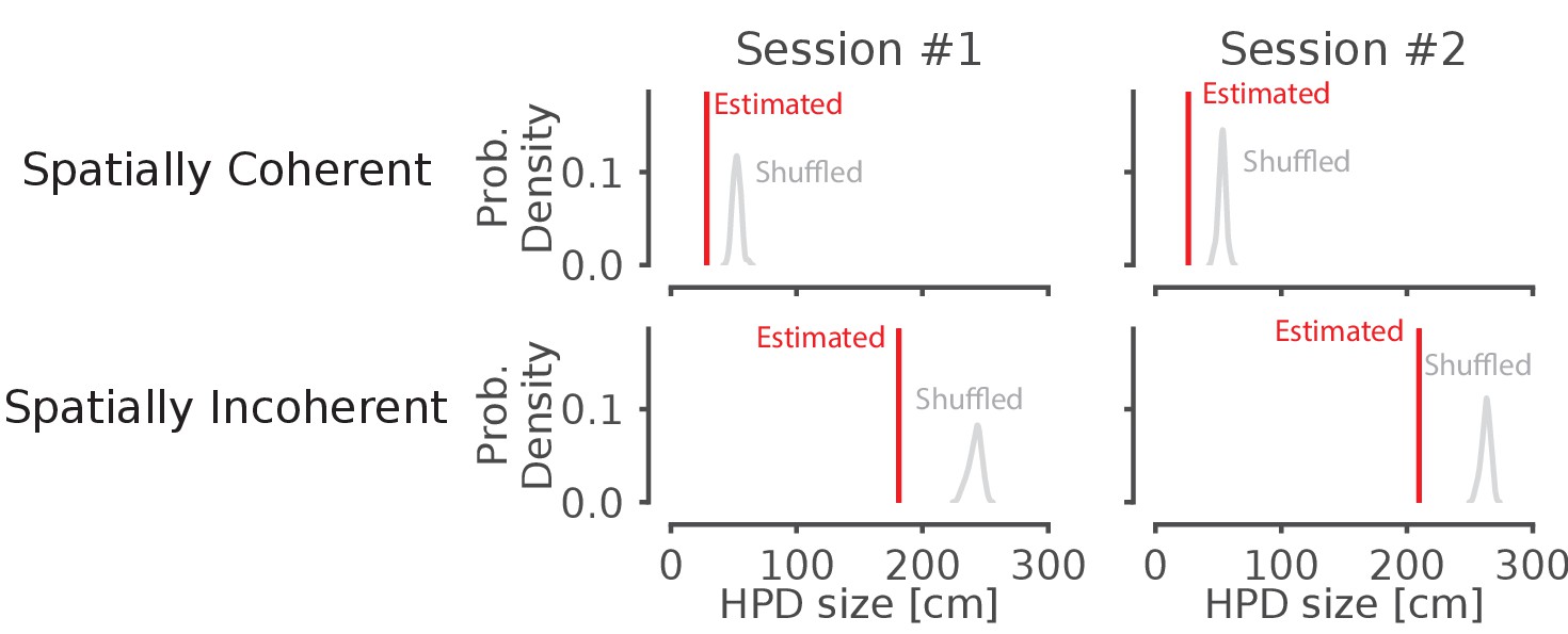
Figure 3—figure supplement 3

Shuffling the data by swapping the runs and circularly permuting the position increases the percentage of spatially incoherent SWRs and decreases the spatially coherent SWRs.
The red line represents the percent of spatially coherent or incoherent SWRs in that recording session for actual data. The histogram represents the distribution after 50 shuffles of the run from well to well as well as the circularly shuffled position (for each tetrode). This preserves local spatial correlations in the data but breaks the global spatial relationships between the spikes and the data.
Figure 3—video 1
Example of an SWR with that is not purely continuous.
Conventions the same as Figure 2—video1.
Figure 4 with 2 supplements
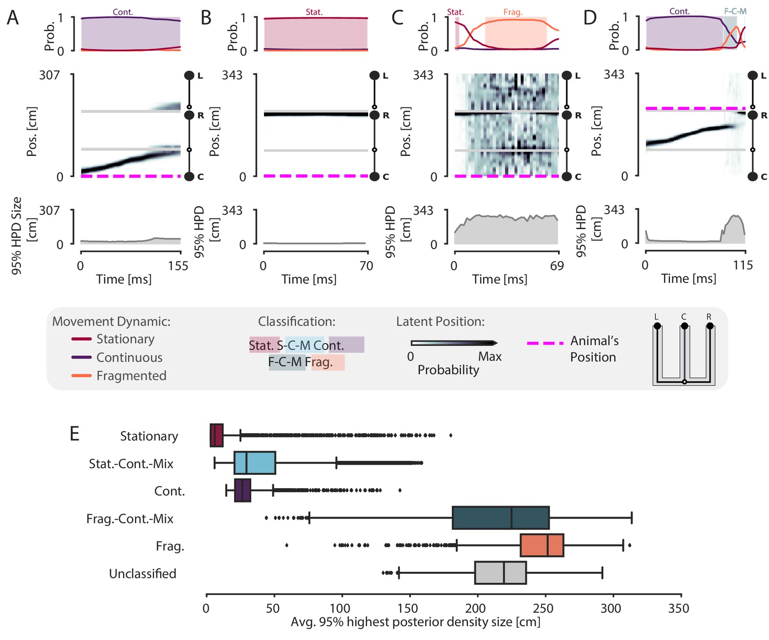
Validation of classification using the 95% Highest Posterior Density.
(A–D) Examples of the 95% Highest Posterior Density. In each column: top panel: Probability of dynamic over time. Shading and labels indicate dynamic categories. Middle panel: Posterior distribution of estimated linear position over time. Magenta dashed line indicates animal’s position. Bottom panel: HPD region size—the integral of the position bins with the top 95% probable values. (E) Average 95% HPD region size for each dynamic category. Median 24 cm for spatially coherent vs. median 238 cm for spatially incoherent, p=2.2e-16, one-sided Mann-Whitney-U.
-
Figure 4—source data 1
Table of replay statistics for each SWR for Figure 4E.
- https://cdn.elifesciences.org/articles/64505/elife-64505-fig4-data1-v2.csv
Figure 4—figure supplement 1
Shuffling the position with replacement increases the average 95% HPD region size.
Red line represents the average 95% HPD region size for all ripples. The histogram represents the distribution after 50 shuffles of the position data. Position data was shuffled by resampling with replacement from the set of all observed positions in that recording session, destroying position information but preserving spiking timing and position occupancy.
Figure 4—figure supplement 2
Shuffling the position data by swapping the runs and circularly permuting the data increases the average 95% HPD region size for spatially coherent and incoherent classified times.
Data from two recording sessions from different animals. Red line represents the average spatial position spanned by the highest posterior density on real data for all ripples. The histogram represents the distribution after 50 shuffles of the position data. The histogram represents the distribution after 50 shuffles of the run from well to well as well as the circularly shuffled position (for each tetrode). This preserves local correlations between spikes but reduces global spatial structure.
Figure 5 with 4 supplements
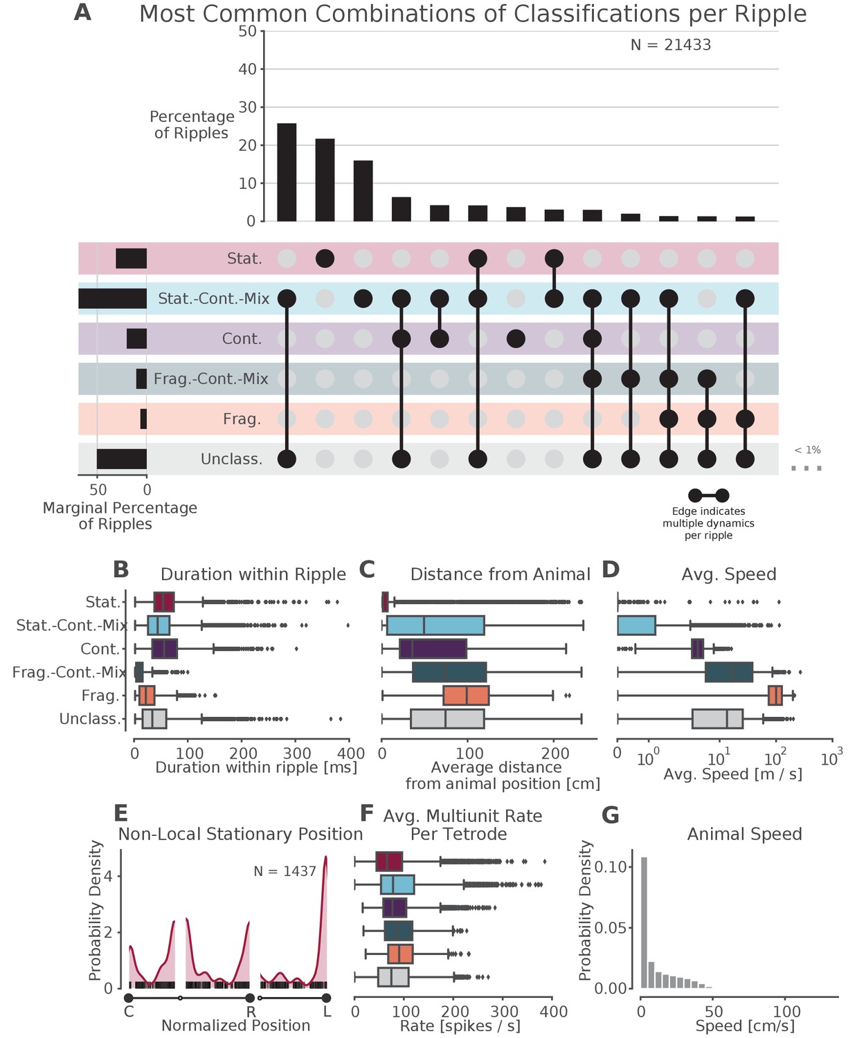
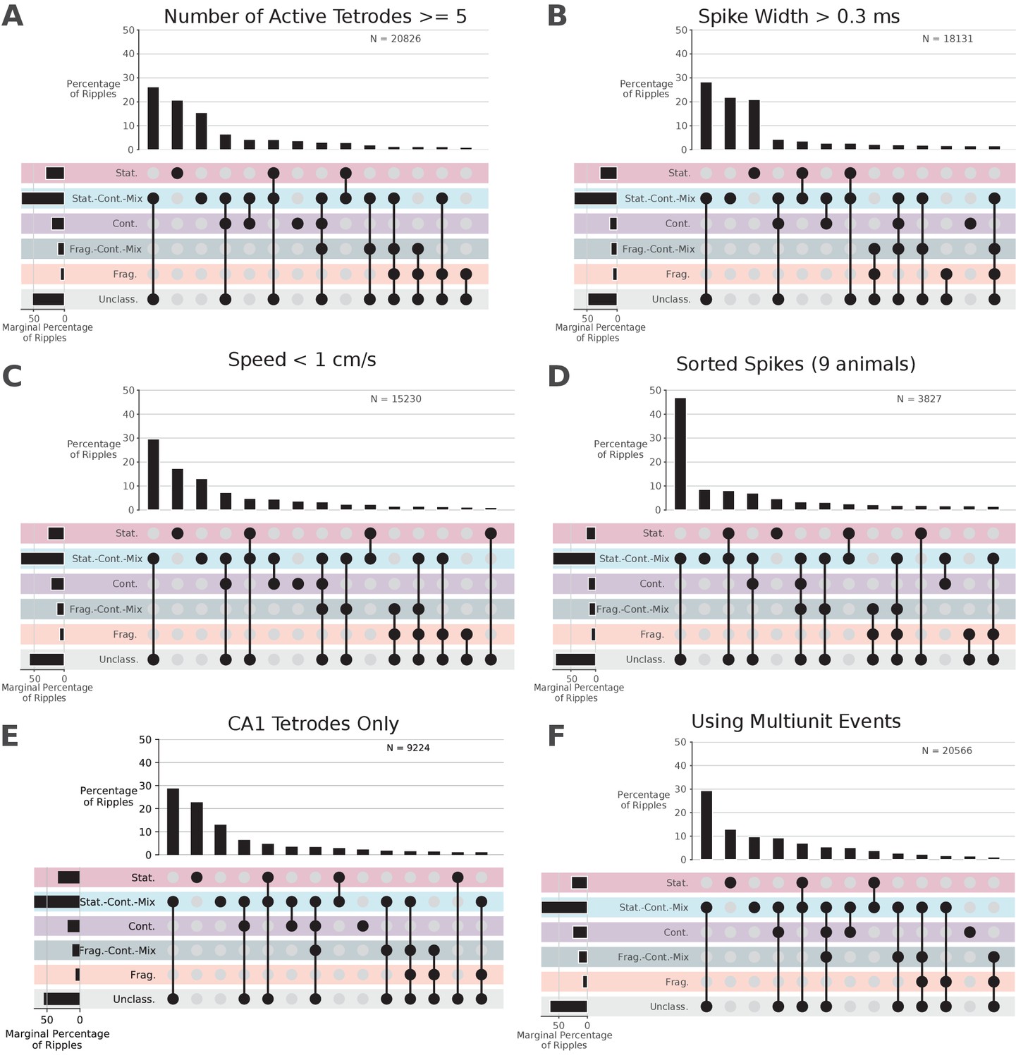
Prevalence of classifications.
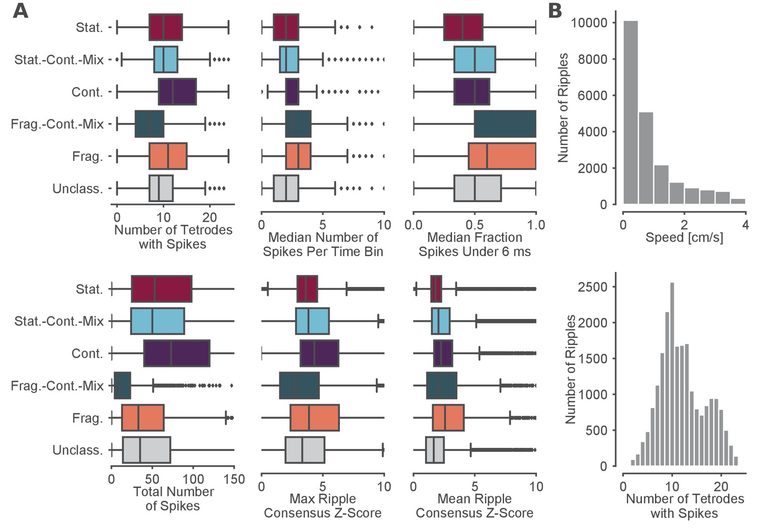
(A) UpSet plot (Lex et al., 2014)—which is similar to a Venn diagram with more than three sets—of the most common sets of classifications within each SWR. Each row represents a classification and each column represents a set of classifications, where filled-in black dots with an edge between the dots indicates that multiple classifications are present in the SWR (at different times). The sets are ordered by how often they occur as indicated by the bar plot above each category. The total percentage of each classification is indicated by the rotated bar plot on the left. (B) Duration of each dynamic category within a SWR. The box shows the interquartile range (25–75%) of the data and the whiskers are 1.5 times the interquartile range. Outlier points outside of this are labeled as diamonds. (C) Average distance between the latent position and the animal’s actual position for each classification within the SWR. (D) Average speed of the classification within the SWR (excluding classifications with durations less than 20 ms). Note that these speeds are calculated using the most probable position (MAP estimate) which can be noisy when the probability of position is flat or multimodal.(E) Kernel density estimate of the position of stationary trajectories on the W-track at least 30 cm away from the animal’s position. The shaded region represents the density estimate while the black ticks represent the observed non-local stationary positions. (F) Average tetrode multiunit spike rates for each dynamic category within each SWR (excluding classifications 20 ms). (G) Probability density of animal movement speeds, illustrating prevalence of slower speed real-world movement consistent with stationary and stationary-continuous mixture replay events.
-
Figure 5—source data 1
Table of replay statistics for each SWR for Figure 5.
- https://cdn.elifesciences.org/articles/64505/elife-64505-fig5-data1-v2.csv
Figure 5—figure supplement 1
More examples of stationary-continuous-mixtures.
Conventions are the same as in Figure 3.
Figure 5—figure supplement 2
Control analyses for distribution of dynamics.
Conventions are the same as in Figure 5.
Figure 5—figure supplement 3
Further quantification of spiking and ripple properties by dynamic.
(A) Further quantification of the dynamics with respect to the spiking and ripple properties. (B) Speed and number of tetrodes with spikes for entire SWR.
Figure 5—video 1
Example of a stationary-continuous-mixture.
Conventions the same as Figure 2—video1.
Figure 6 with 2 supplements
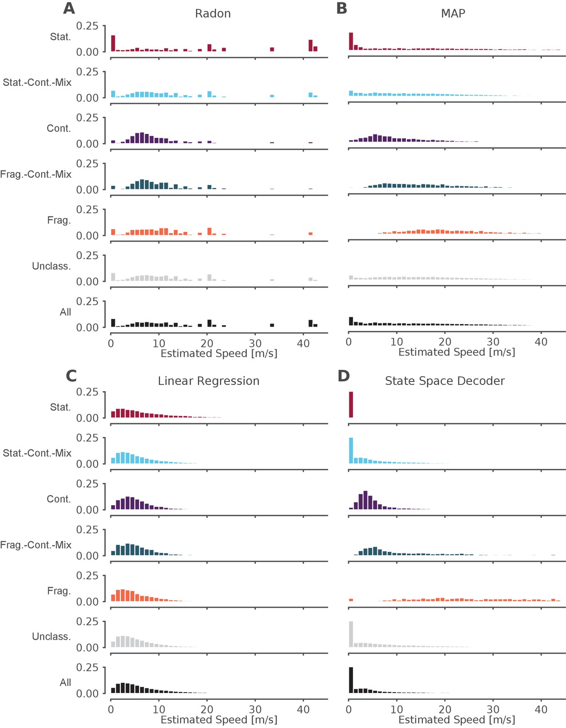
The standard decoder MAP estimate speeds are the most similar to the state space decoder.
Event speeds calculated using three common 'Bayesian' decoder approaches (A–C) compared to using the state space model (D). For each panel, the top five rows show the probability density of the estimated speed for SWRs that contain that dynamic or combination of dynamics. Note that these categories are not mutually exclusive since a SWR can include more than one dynamic or combination of dynamics. The sixth row shows all SWRs containing unclassified dynamics. The final row is the estimated speed for all SWRs. (A) Radon transform (B) MAP estimate (C) Linear regression (D) State space decoder presented in this manuscript.
-
Figure 6—source data 1
Table of replay statistics for each SWR for Figure 6.
- https://cdn.elifesciences.org/articles/64505/elife-64505-fig6-data1-v2.csv
Figure 6—figure supplement 1
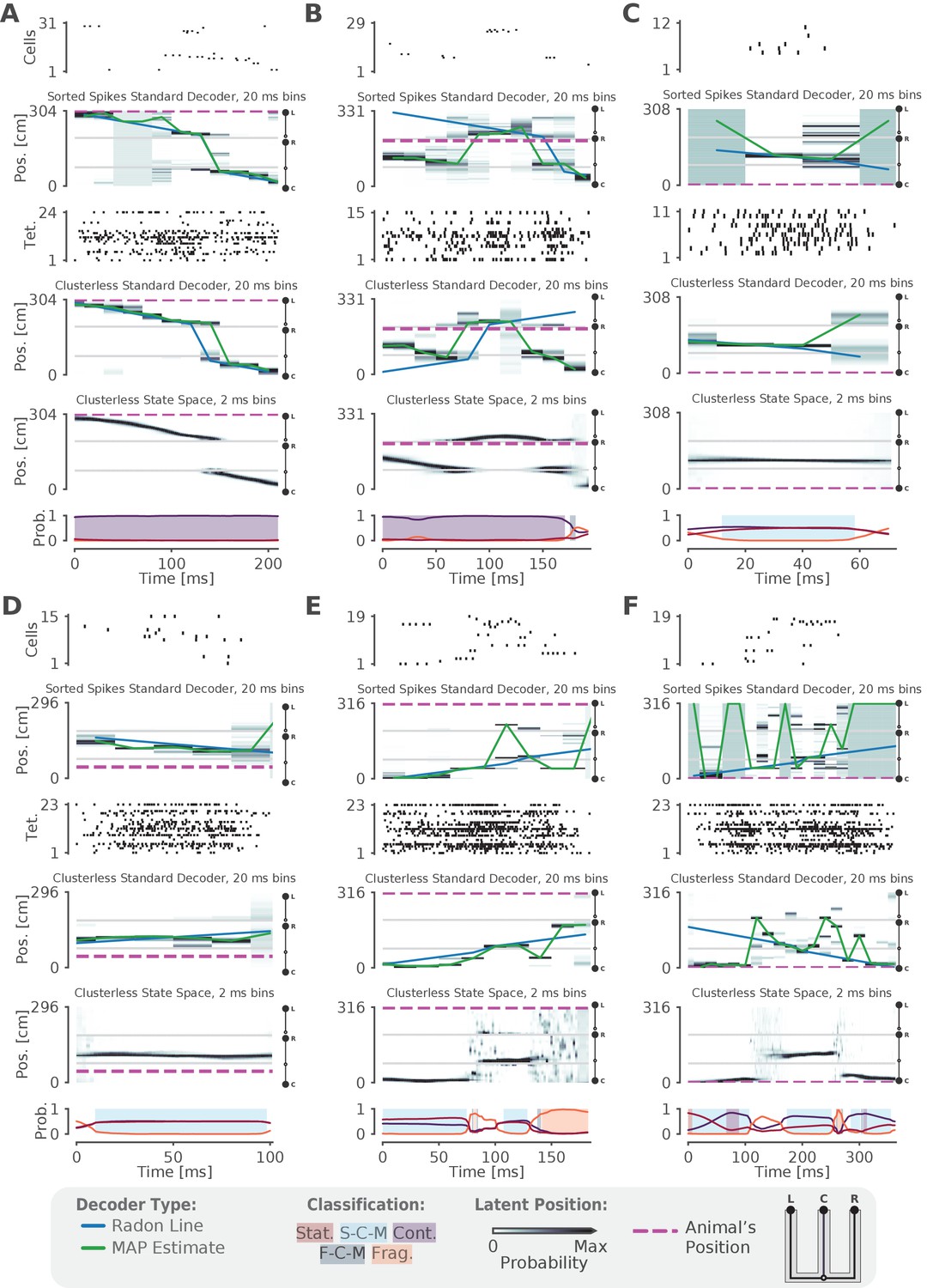
Examples of fits from the standard 'Bayesian' decoder with 20 ms bins and state space model.
(A–F) For each panel, the top row is a raster plot of the sorted cells, the second row is the decoded posterior probability of position in 20 ms time bins for the sorted spikes and the corresponding Radon line fit (blue line) and the MAP fit (green line) on this posterior probability, the third row is a raster plot of the multiunit spike times used for clusterless decoding, the fourth row is the posterior probability in 20 ms time bins using clusterless data as well as the accompanying Radon fit and MAP fit, the fifth row is the posterior probability from the clusterless state space model, and the sixth row is the probability of each dynamic (lines) and the color shading indicates the category of dynamic as before.
Figure 6—figure supplement 2
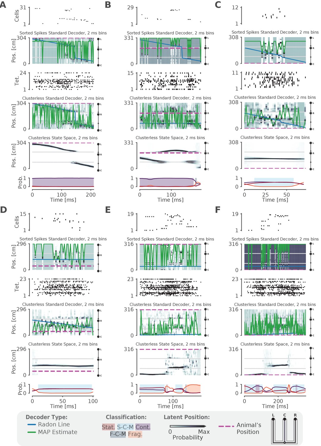
Examples of fits from the standard 'Bayesian' decoder with 2 ms bins and state space model.
(A–F) For each panel, the top row is a raster plot of the sorted cells, the second row is the decoded posterior probability of position in 2 ms time bins for the sorted spikes and the corresponding Radon line fit (blue line) and the MAP fit (green line) on this posterior probability, the third row is a raster plot of the multiunit spike times used for clusterless decoding, the fourth row is the posterior probability in 2 ms time bins using clusterless data as well as the accompanying Radon fit and MAP fit, the fifth row is the posterior probability from the clusterless state space model, and the sixth row is the probability of each dynamic (lines) and the color shading indicates the category of dynamic as before.
Author response image 1
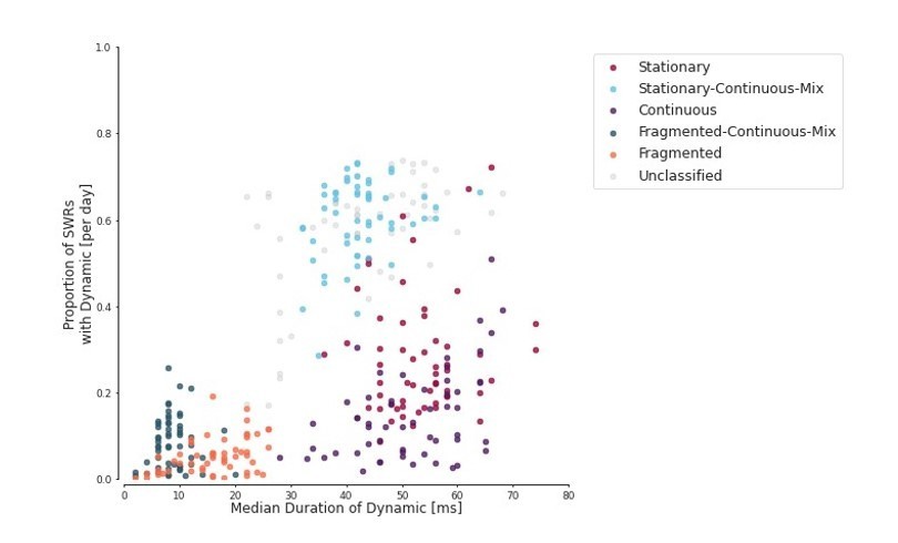
Proportion of SWRs for each day vs duration of the dynamic within the SWR.
Each dot represents one day for one animal.
Author response image 2
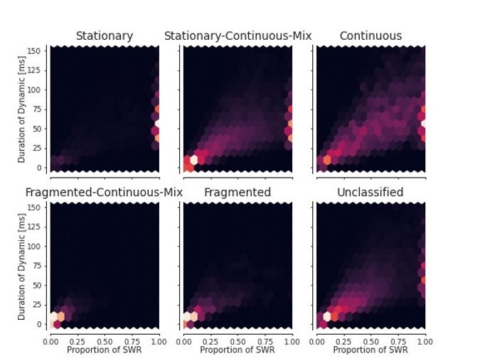
For each dynamic, the duration of the dynamic vs the proportion of time of the total SWR duration.
Additional files
Download links
A two-part list of links to download the article, or parts of the article, in various formats.
Downloads (link to download the article as PDF)
Open citations (links to open the citations from this article in various online reference manager services)
Cite this article (links to download the citations from this article in formats compatible with various reference manager tools)
Hippocampal replay of experience at real-world speeds
eLife 10:e64505.
https://doi.org/10.7554/eLife.64505


