Robust vestibular self-motion signals in macaque posterior cingulate region
- CAS Center for Excellence in Brain Science and Intelligence Technology, Key Laboratory of Primate Neurobiology, Institute of Neuroscience, Chinese Academy of Sciences, China
- University of Chinese Academy of Sciences, China
Figures
Figure 1
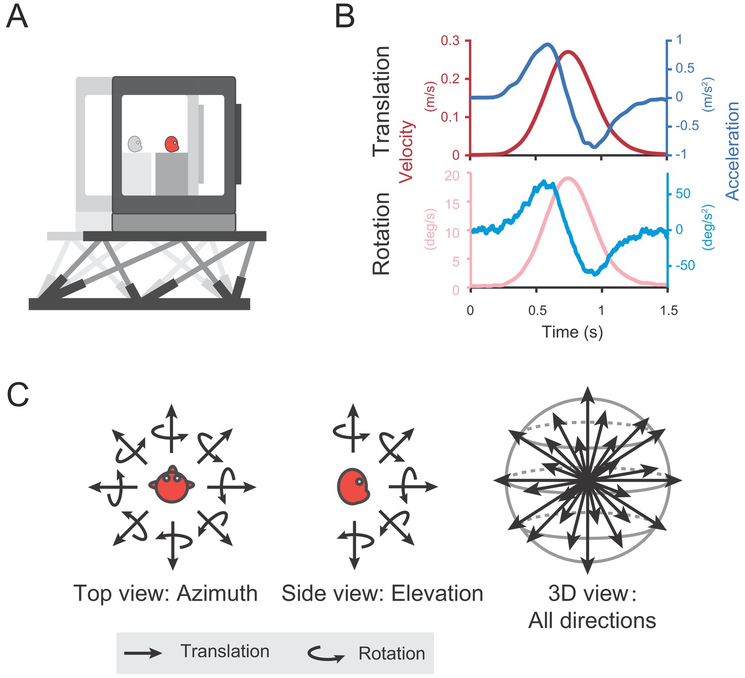
Diagram of experimental set-up.
(A) Monkeys were translated or rotated by a 6-degree-of-freedom motion platform (MOOG). A visual display is mounted on the platform, providing visual stimuli that simulate real motion. (B) Motion profiles. For translation, acceleration (dark blue) signals were collected from an accelerometer mounted on the platform and velocity quantity (dark red) is an integral from the acceleration. For rotation, velocity (light red) signals were collected from a gyroscope mounted on the platform and acceleration (light blue) is the derivative from the velocity. Stimulus duration is 1.5 s. (C) Illustration of 26 motion vectors in 3D space under translation (straight arrow) and rotation (curved arrow) conditions. Left panel indicates the eight equally distributed directions in the horizontal plane from the top view. Middle panel shows five equally distributed directions in the vertical plane from the side view.
Figure 2
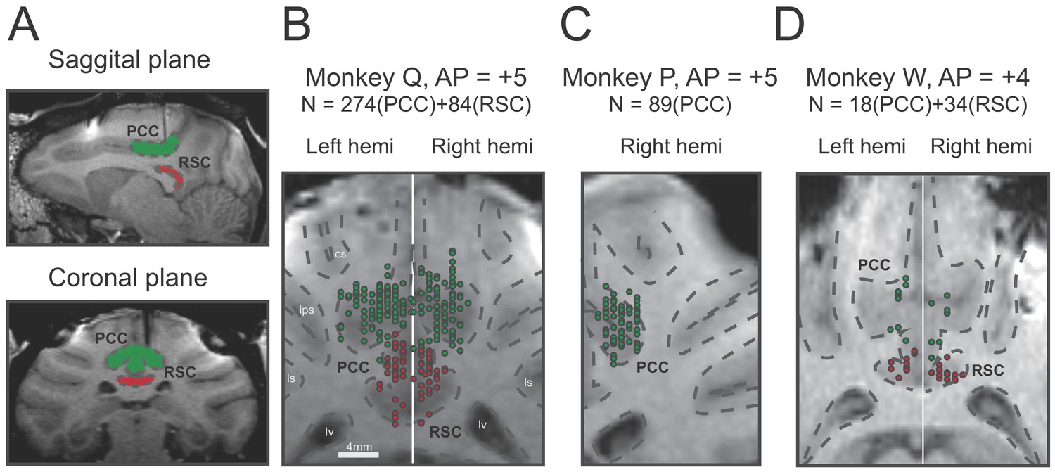
Recording sites reconstructed on MRI images of three monkeys.
(A) Sagittal and coronal planes in one animal (monkey Q), with green shaded areas indicating PCC and red shaded areas indicating RSC. Electrode penetration is indicated by the dark shaded lines. (B–C). Recording sites are reconstructed and superimposed onto one plane in each of the three animals. RSC, retrosplenial cortex; PCC, posterior cingulate cortex; cs, central sulcus; ips, intraparietal sulcus; ls, lateral sulcus; lv, lateral ventricle.
Figure 3 with 2 supplements
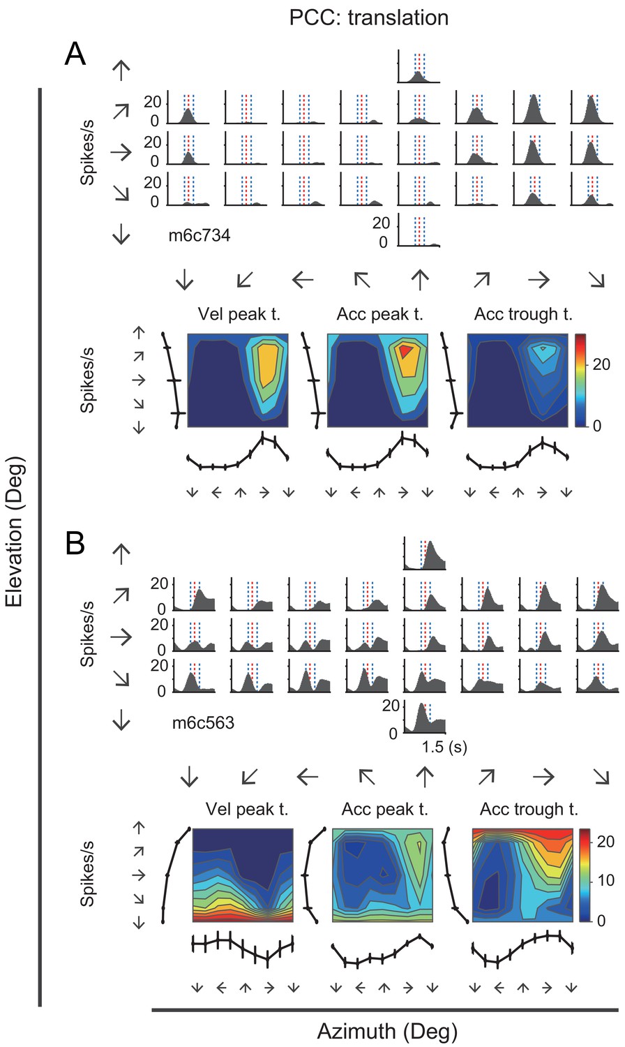
PSTHs from two example neurons in the vestibular condition.
(A) Upper panels: PSTHs of an example PCC velocity-dominant neuron across 26 directions under the translation condition. The red dashed lines indicate the velocity peak time of velocity profile and the two blue dashed lines indicate the peak time of acceleration peak and trough. Bottom panels: Contour figures show firing rates as a function of azimuth and elevation at three different time points (velocity peak time, acceleration peak and trough, respectively). (B) Upper panels: PSTHs of an example acceleration-d neuron under the translation condition. Bottom panels: Contour figures of this neuron.
Figure 3—figure supplement 1
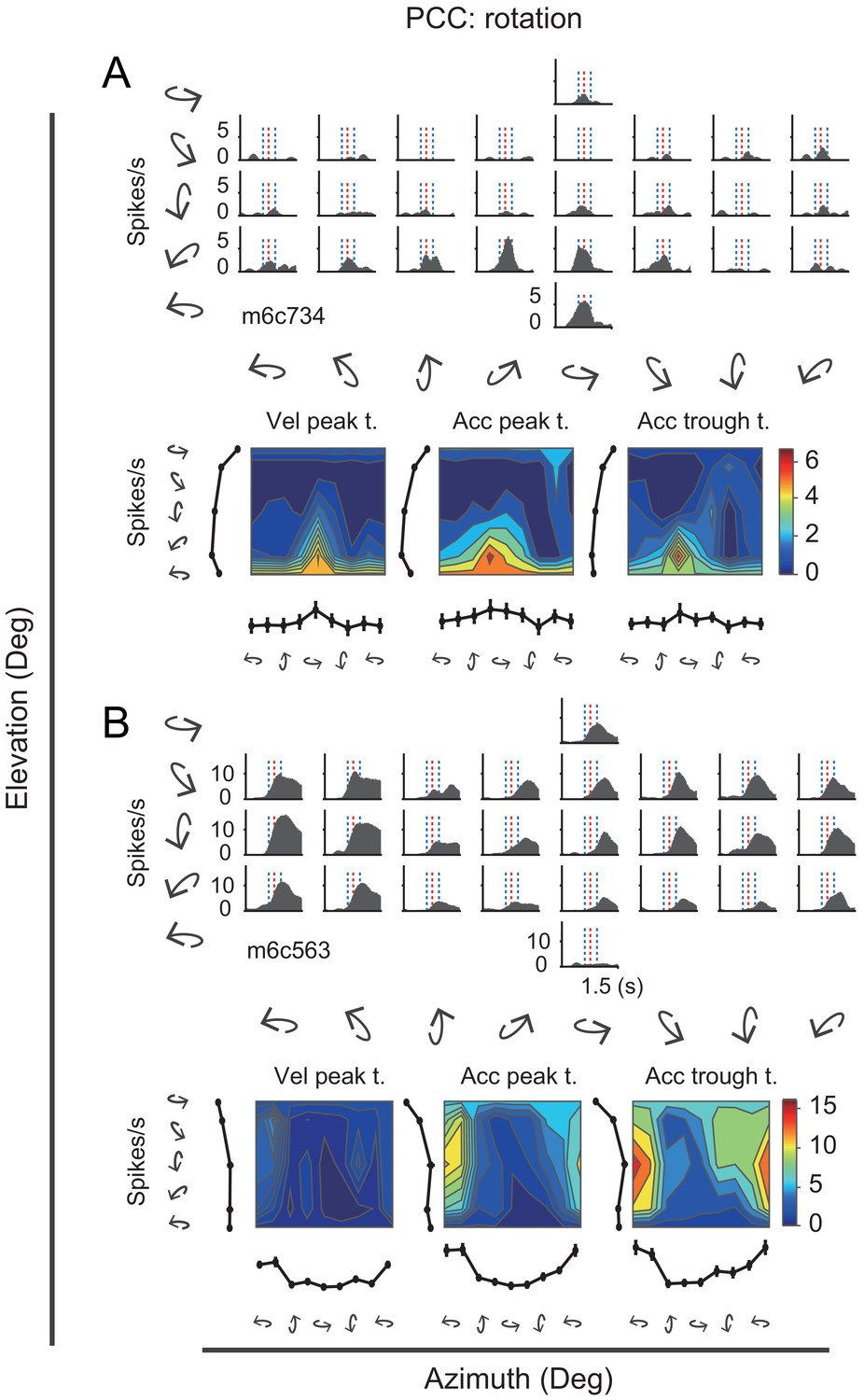
PSTHs from the same two example neurons under rotation condition.
(A) Upper panels: PSTHs of the velocity-dominant neuron across 26 directions. The red dashed lines indicate the velocity peak time of velocity profile and the two blue dashed lines indicate the peak time of acceleration peak and trough. Bottom panels: Contour figures show firing rates as a function of azimuth and elevation at three different time points (velocity peak time, acceleration peak and trough, respectively). (B) PSTHs and contour figures of the acceleration-dominant neuron.
Figure 3—figure supplement 2

PSTHs from two example neurons in RSC.
(A) Upper panels: PSTHs of an example neuron across 26 directions under translation condition. The red dashed lines indicate the velocity peak time of velocity profile and the two blue dashed lines indicate the peak time of acceleration peak and trough. Bottom panels: Contour figures show firing rates as a function of azimuth and elevation at three different time points (velocity peak time, acceleration peak and trough, respectively). (B) PSTHs and contour figures of another example neuron under rotation condition.
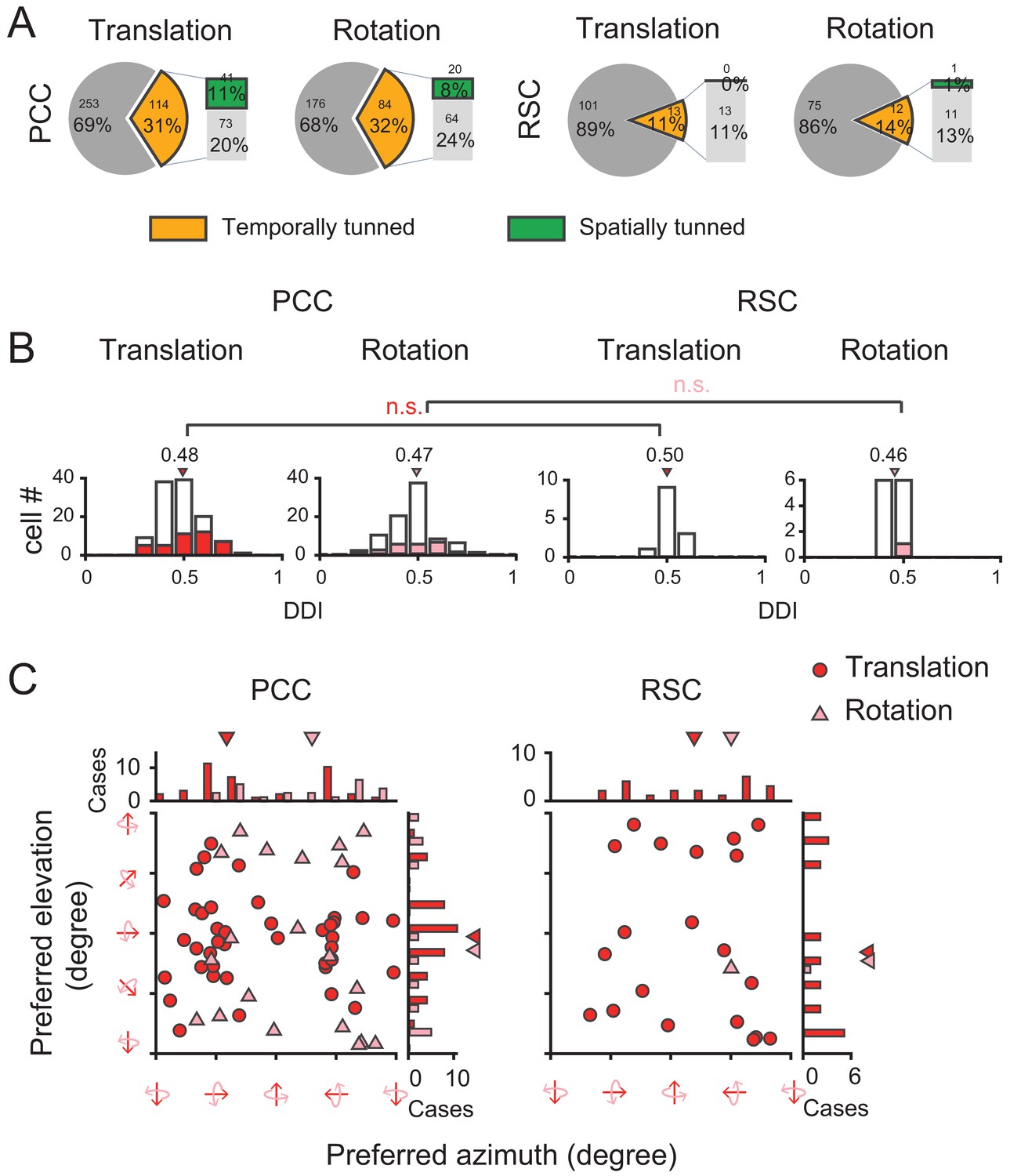
Figure 4 with 2 supplements
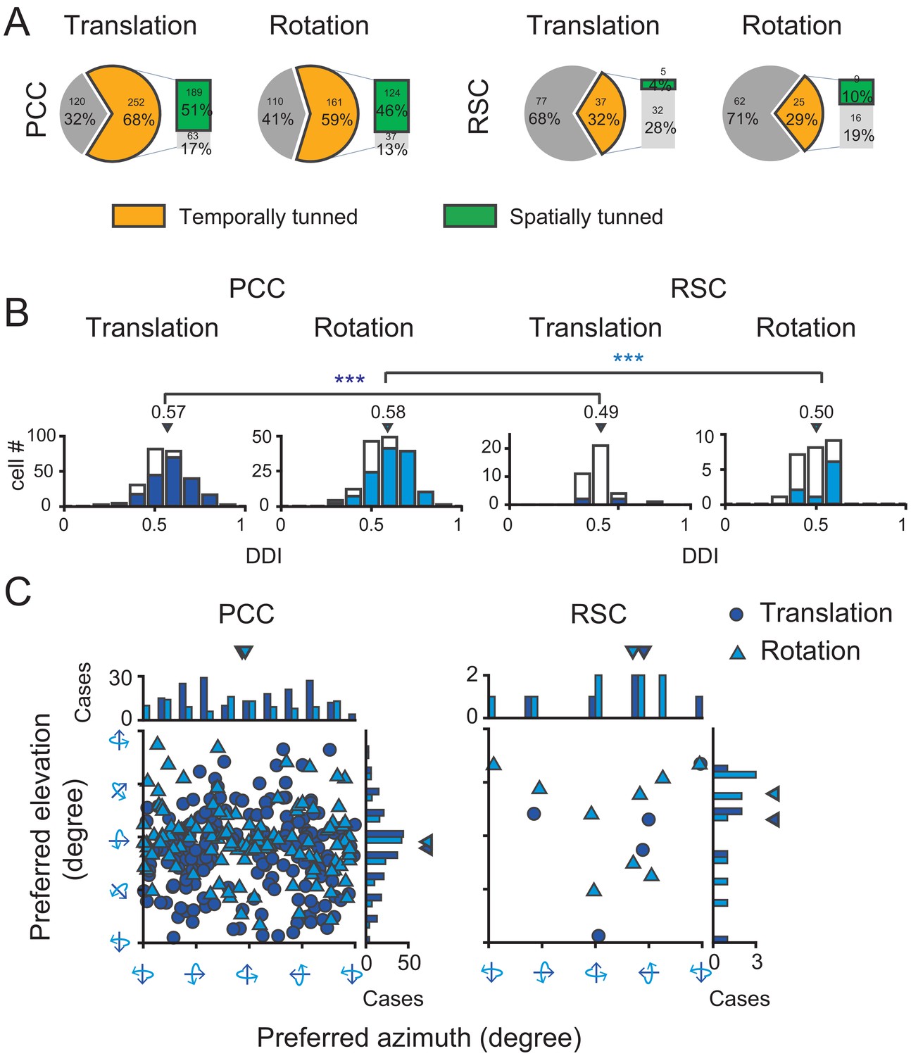
Population summary of temporal and spatial tuning properties of vestibular signals in PCC and RSC.
(A). Proportion of neurons in each category. (B) DDI distribution of neurons with significant temporal tuning. Filled bars indicate neurons with significant spatial tuning. (C) Distribution of preferred directions for neurons with significant spatial tuning. Dark blue symbol: translation condition; Light blue symbol: rotation condition.
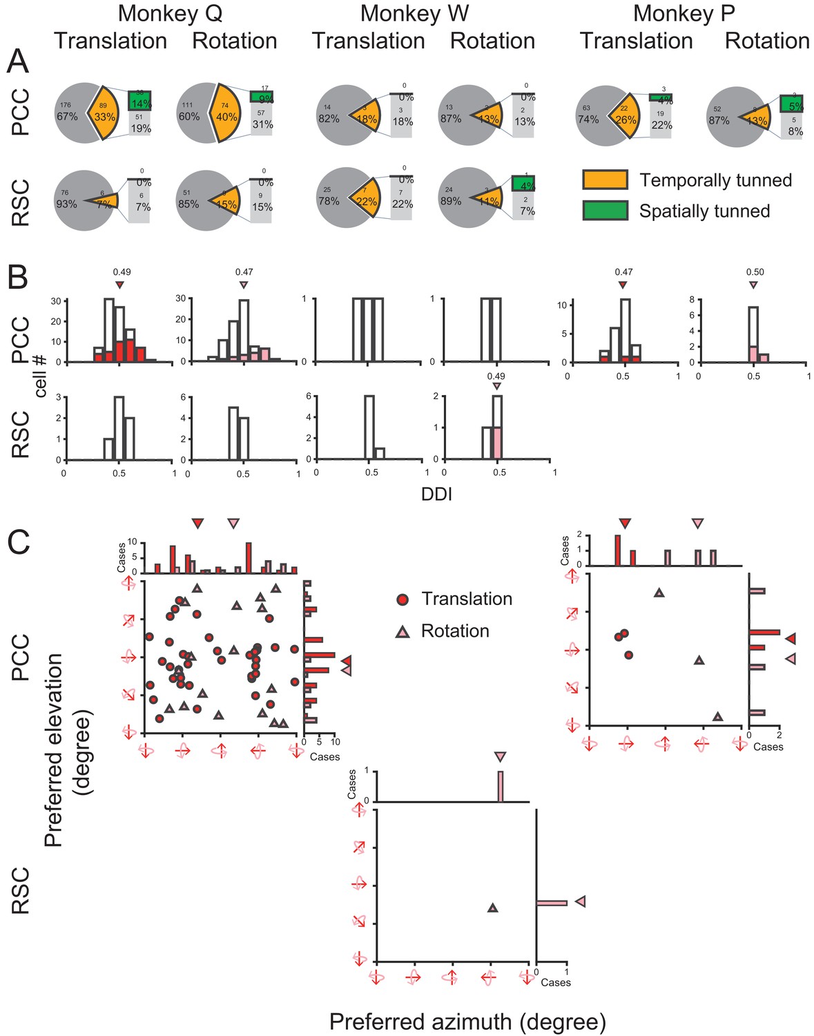
Figure 4—figure supplement 1
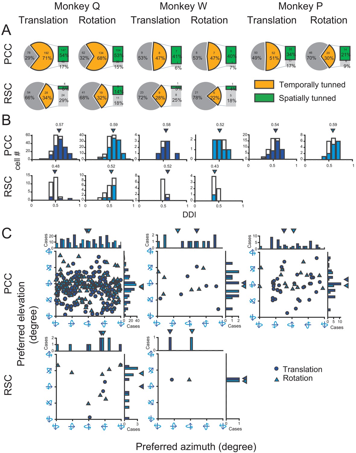
Population summary of temporal and spatial tuning properties of vestibular signals according to the three monkeys.
(A). Proportion of neurons in each category. (B) DDI distribution of neurons with significant temporal tuning. Filled bars indicate neurons with significant spatial tuning. (C) Distribution of preferred directions for neurons with significant spatial tuning. Dark blue symbol: translation condition; Light blue symbol: rotation condition. Note that RSC neurons were not recorded form monkey P.
Figure 4—figure supplement 2
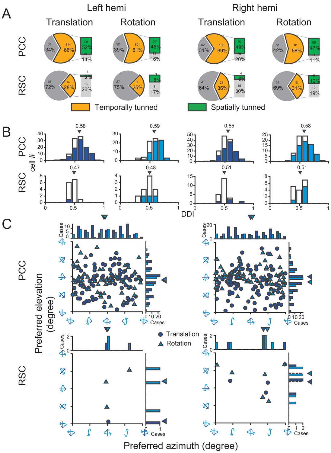
Population summary of temporal and spatial tuning properties of vestibular signals according to left and right hemispheres.
(A). Proportion of neurons in each category. (B) DDI distribution of neurons with significant temporal tuning. Filled bars indicate neurons with significant spatial tuning. (C) Distribution of preferred directions for neurons with significant spatial tuning. Dark blue symbol: translation condition; Light blue symbol: rotation condition.
Figure 5
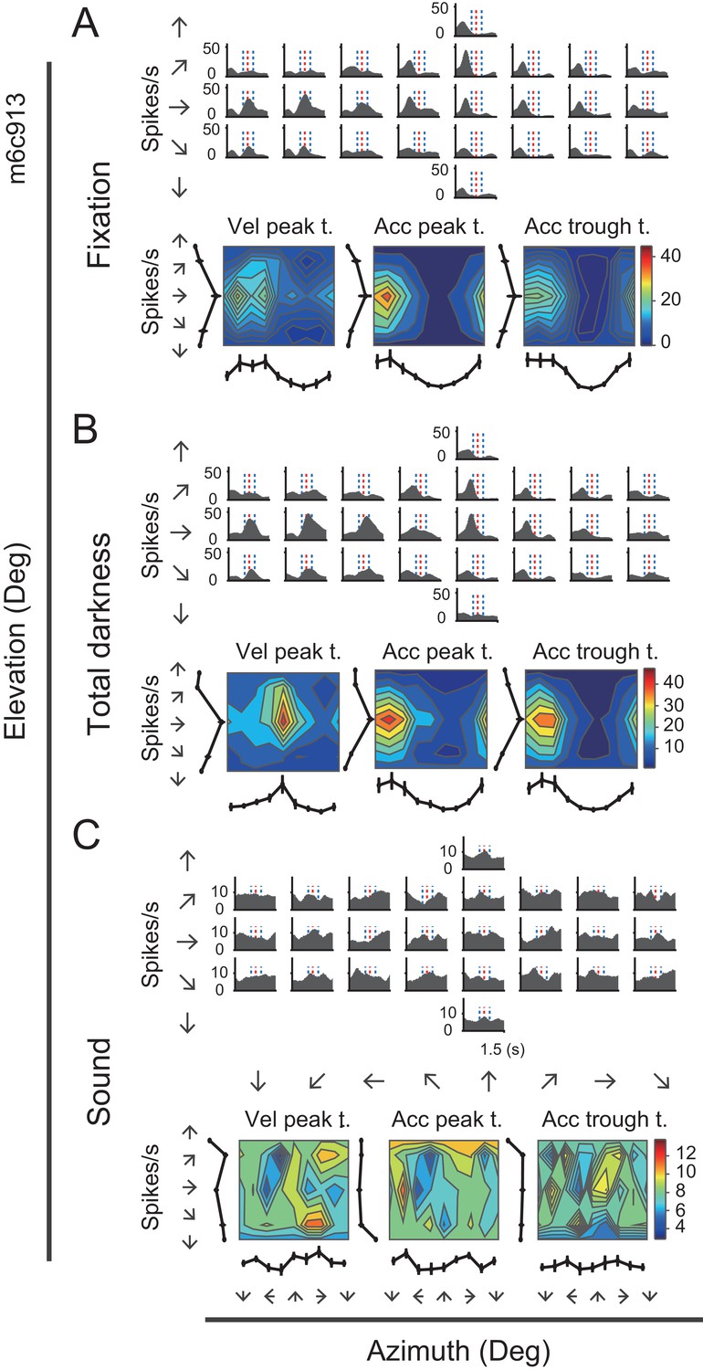
Neural activity of an example neuron in total darkness and sound conditions.
(A–C) Responses from an example cell in the regular vestibular translation condition (A), total darkness condition (B), and sound control condition (C).
Figure 6
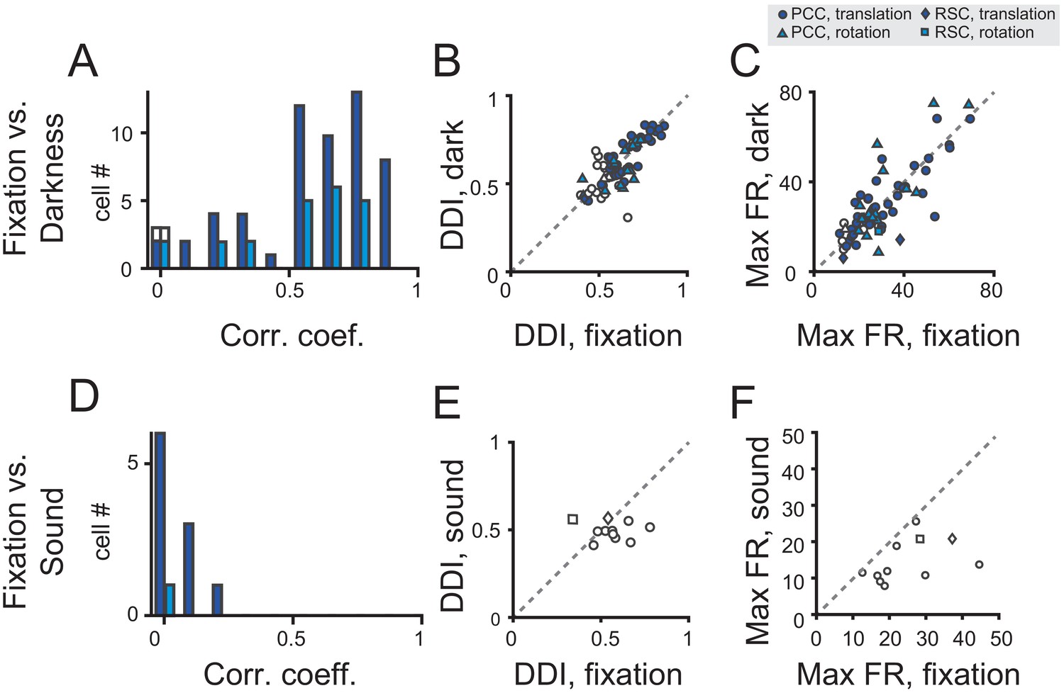
Population analysis in total darkness and sound conditions.
(A–C) Pearson correlation coefficient of PSTHs (A), DDI (B), maximum firing rate (C) between regular vestibular and total darkness conditions. Filled symbols indicate neurons with significant spatial tuning, whereas open symbols indicate neurons without significant spatial tuning in either stimuli condition. Dark blue symbol: translation condition; Light blue symbol: rotation condition. (D–E) Pearson correlation coefficient of PSTHs (D), DDI (E), maximum firing rate (F) between regular vestibular and sound control condition.
Figure 7 with 1 supplement

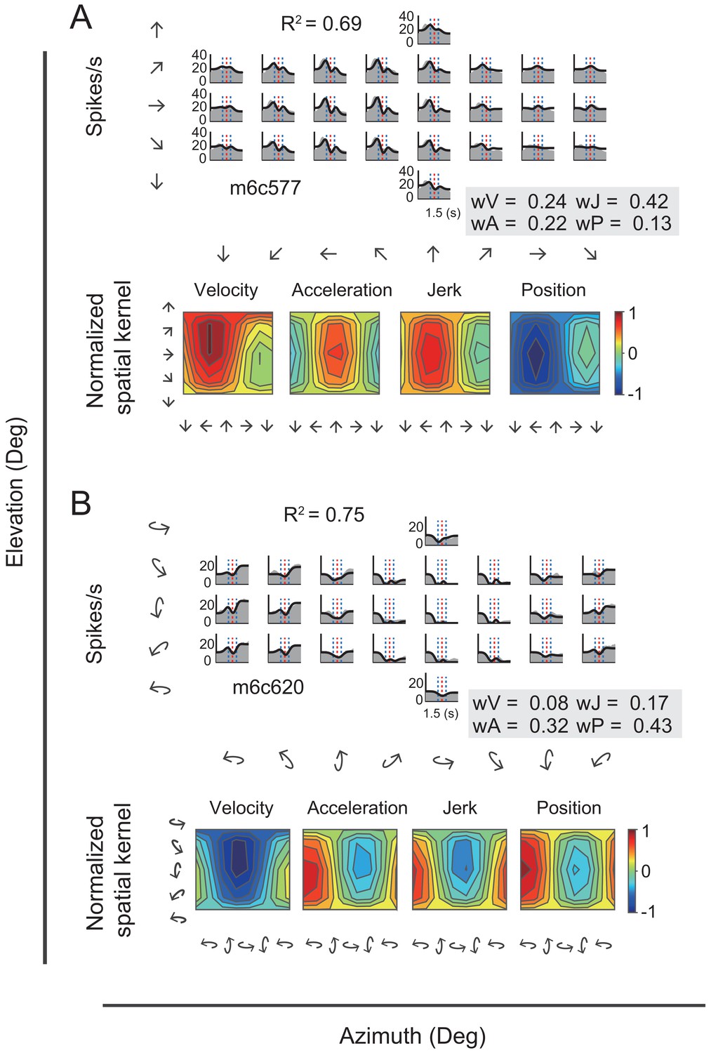
Fitting results of two example neurons with VA model.
(A–B) Upper panels: PSTHs of two example cells fitted by VA model. Gray areas are PSTHs and superimposed black lines are fitted data. Red dashed lines: peak time of velocity; Blue dashed lines: peak and trough time of acceleration. The fitted weight of velocity and acceleration are shown in the gray box. These two examples are the same neurons shown in Figure 3. Lower panels: Contour figures of spatial kernels of the velocity and acceleration components.
Figure 7—figure supplement 1
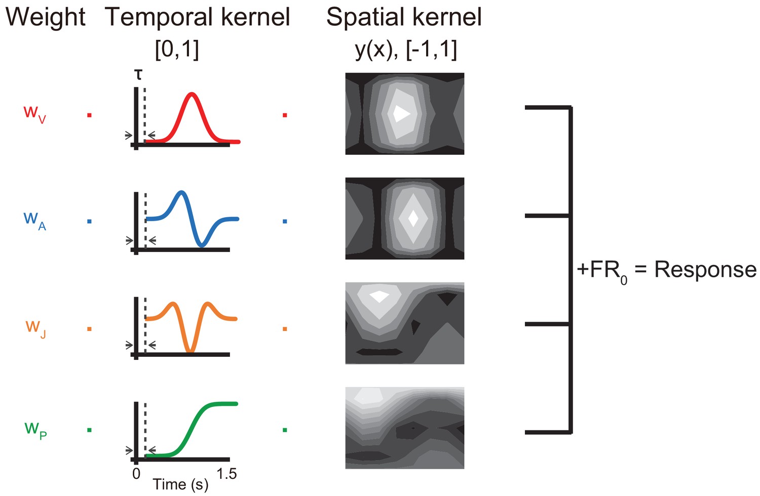
Illustration of the three-dimensional temporal-spatial model.
The full PVAJ model contains four different components, velocity, acceleration, jerk and position, which are summed linearly by their corresponding weights, with their own temporal kernel and spatial kernel. The spatial kernel is cosine function fed through a linear function that was depended on parameters of preferred azimuth and preferred elevation.
Figure 8
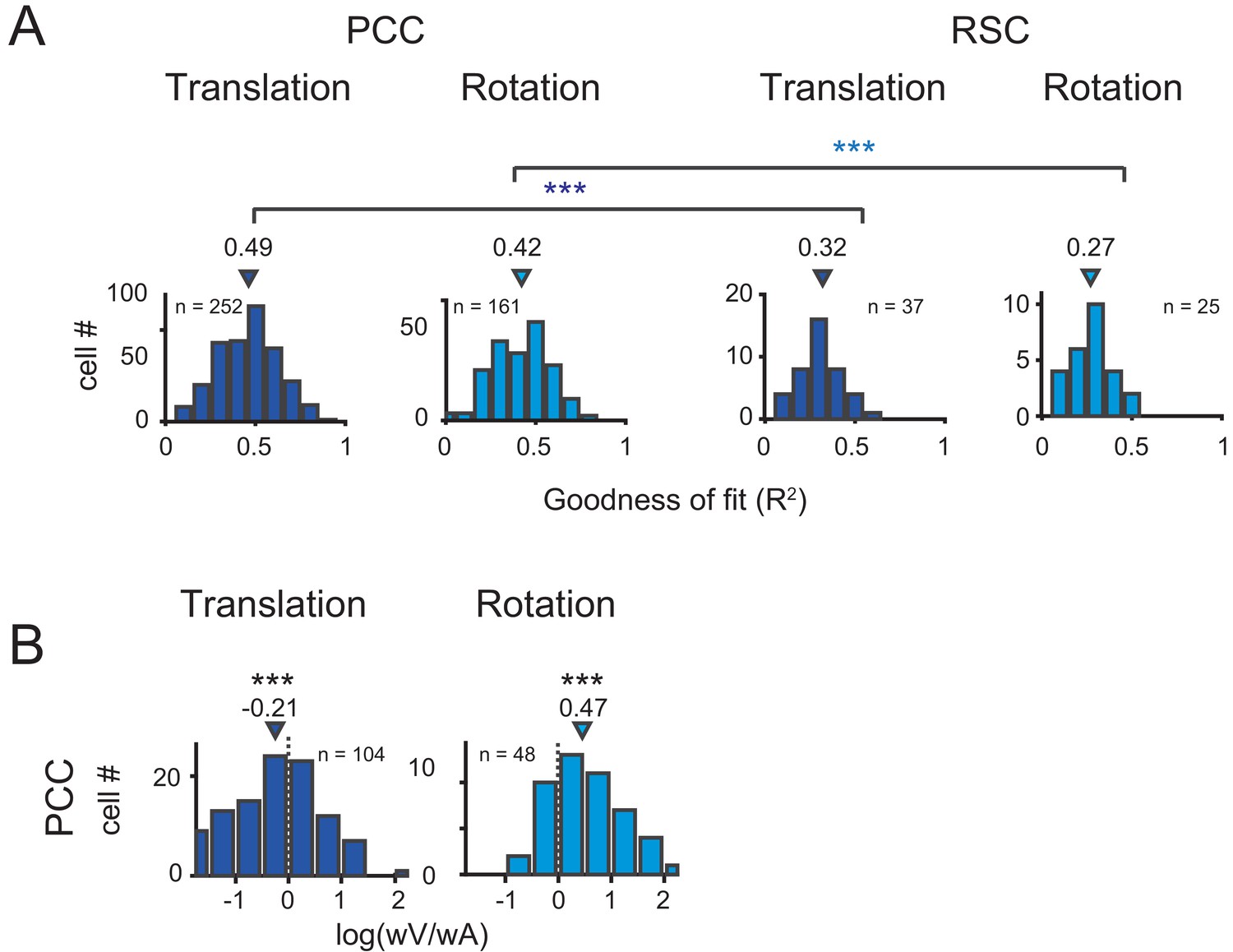
Population results with VA model.
(A) Goodness of fit for PCC and RSC. Triangles are median value of each distribution. (B) Log ratio of the velocity weight to the acceleration weight. Triangles show the median value. Only data with R2 >0.5 were included.
Figure 9
Fitting results of two example neurons with PVAJ model.
(A–B) Upper panels: PSTHs of two example cells fitted by VA model. Gray areas are PSTHs and superimposed black lines are fitted data. Red dashed lines: peak time of velocity; Blue dashed lines: peak and trough time of acceleration. The fitted weight of velocity, acceleration, jerk and position components are shown in the gray box. Lower panels: Contour figures of spatial kernels of the velocity and acceleration components.
Figure 10
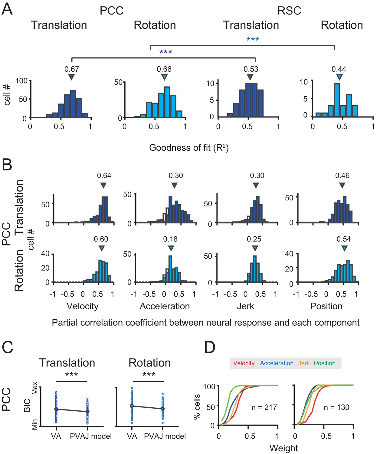
Population results with PVAJ model.
(A) Goodness of fit (R2) from the PVAJ model assessed by Pearson correlation between the experimental and fitted data. Triangles: median value. (B) Distribution of partial correlation coefficient between neuronal response and the fitted data of each temporal component in the full model. Filled bar indicates significance with p<0.05. (C) Comparison of BIC between VA model and PVAJ model. The large blue circles indicate mean value that are superimposed on individual values (small circles). (D) Cumulative distributions of the weight of different signal components. Only data with R2 >0.5 were included.
Figure 11
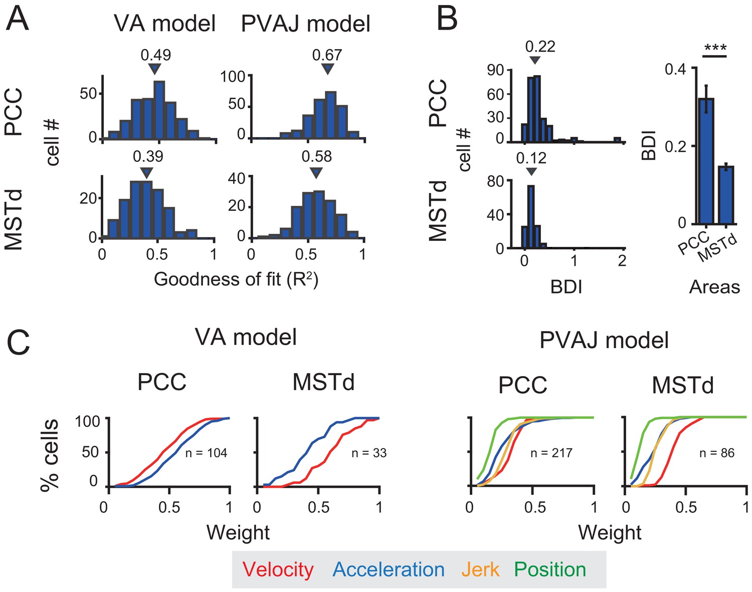
Comparison between PCC and MSTd fitted with VA and PVAJ models.
(A) Distribution of goodness of fit (R2). Triangles: medians. (B) Left column: difference in the BIC (Bayesian Information Criterion) between the two models (BDI, BIC difference index, see Materials and methods). Five cases in PCC with BDI larger than two were cut off at two for sake of illustration. Right column: Comparison of the BDI between PCC and MSTd. Bars are the mean value and the error bars are s.e.m. ***: p=0.00034. (C) Cumulative distributions of the weight of signal component. Only data with R2 >0.5 were included.
Figure 12 with 2 supplements
Visual self-motion signals (optic flow) in the posterior cingulate region.
(A) Proportion of temporal and spatial tuning in PCC and RSC. (B) Distributions of DDI. (C) Preferred direction. Symbol representations are same as in Figure 4.
Figure 12—figure supplement 1

Population summary of temporal and spatial tuning properties of visual signals according to the three monkeys.
(A) Proportion of neurons in each category. (B) DDI distribution of neurons with significant temporal tuning. Filled bars indicate neurons with significant spatial tuning. (C) Distribution of preferred directions for neurons with significant spatial tuning. Dark red symbol: translation condition; Light red symbol: rotation condition. Note that RSC neurons were not recorded form monkey P, and there is no significant spatially tunned PCC neuron in monkey W in translation condition and RSC neuron in monkey Q in rotation condition.
Figure 12—figure supplement 2
Population summary of temporal and spatial tuning properties of visual signals according to left and right hemispheres.
(A). Proportion of neurons in each category. (B) DDI distribution of neurons with significant temporal tuning. Filled bars indicate neurons with significant spatial tuning. (C) Distribution of preferred directions for neurons with significant spatial tuning. Dark red symbol: translation condition; Light red symbol: rotation condition. Note that there is no significant spatially tunned RSC neuron in left hemispheres in rotation condition.
Tables
Table 1
Temporal and spatial tuning properties across subregions of posterior cingulate area under different conditions.
| Subregion | Conditions | Vestibular | Visual | ||
|---|---|---|---|---|---|
| Temporally tuned | Spatially tuned | Temporally tuned | Spatially tuned | ||
| PCC | Translation | 252/372 (68%) | 189/252 (75%) | 114/367 (31%) | 41/114 (36%) |
| Rotation | 161/271 (59%) | 124/161 (77%) | 84/260 (32%) | 20/84 (24%) | |
| RSC | Translation | 37/114 (32%) | 5/37 (14%) | 13/114 (11%) | 0/13 (0%) |
| Rotation | 25/87 (29%) | 9/25 (36%) | 12/87 (14%) | 1/12 (1%) | |
Table 2
Temporal and spatial tuning properties under total darkness and sound control experiments.
Note in the sound control conditions, there is no neuron with significant temporal tuning, so we did not calculate the spatial tuning properties.
| Conditions | Dark control | Sound control | ||
|---|---|---|---|---|
| Temporally tuned | Spatially tuned | Temporally tuned | Spatially tuned | |
| Translation | 42/49 (86%) | 34/43 (79%) | 0/10 (0%) | / |
| Rotation | 16/18 (89%) | 15/16 (94%) | 0/1 (0%) | / |
Additional files
Download links
A two-part list of links to download the article, or parts of the article, in various formats.
Downloads (link to download the article as PDF)
Open citations (links to open the citations from this article in various online reference manager services)
Cite this article (links to download the citations from this article in formats compatible with various reference manager tools)
Robust vestibular self-motion signals in macaque posterior cingulate region
eLife 10:e64569.
https://doi.org/10.7554/eLife.64569


