Value representations in the rodent orbitofrontal cortex drive learning, not choice
- Princeton Neuroscience Institute, Princeton University, United States
- DeepMind, United Kingdom
- Department of Ophthalmology, University College London, United Kingdom
- Gatsby Computational Neuroscience Unit, University College London, United Kingdom
- Howard Hughes Medical Institute and Department of Molecular Biology, Princeton University, United States
Figures
Figure 1
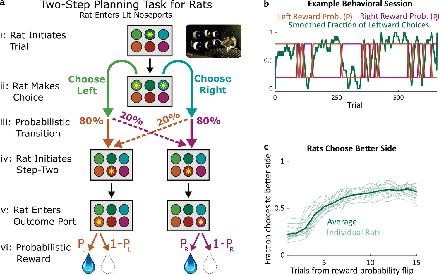
Two-step task for rats.
(a) Rat two-step task. The rat initiates a trial by entering the top center port (i), then chooses to enter one of two choice ports (ii). This leads to a probabilistic transition (iii) to one of two possible paths. In both paths, the rat enters the bottom center port (v), causing one of two outcome ports to illuminate. The rat enters that outcome port (v), and receives a reward (vi). (b) Example behavioral session. At unpredictable intervals, outcome port reward probabilities flip synchronously between high (80%) and low (20%). The rat adjusts choices accordingly. (c) The fraction of trials on which each rat (n=19) selected the choice port whose common (80%) transition led to the outcome port with the currently higher reward probability, as a function of the number of trials that have elapsed since the last reward probability flip.
Figure 2 with 2 supplements
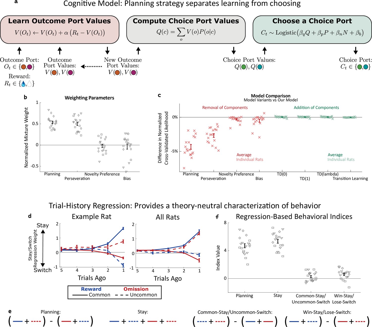
Planning strategy separates learning, choosing.
(a) Schematic of the planning strategy. Agent maintains value estimates (V) for each outcome port, based on a history of recent rewards at that port; as well as value estimates (Q) for each choice port, which are computed on each trial based on the outcome values and the world model (P(o|c)). Choices are drawn probabilistically, based on a weighted combination of these values and of the influence of three other behavioral patterns: perseveration, novelty preference, and bias (see Methods for details). (b): Mixture weights of the different components of the cognitive model fit to rats’ behavioral data. shown for electrophysiology rats (n=6, squares), optogenetics rats (n=9, triangles), and sham optogenetics rats (n=4, diamonds). (c) Change in quality of model fit resulting from removing components from the model (red) or adding additional components (green). (d) Fit weights of the trial-history regression for an example rat (left) and averaged over all rats (right). (e) Definitions of the four behavioral indices in terms of the fit stay/switch regression weights. The planning index for a particular rat is defined as the sum of that rat’s common-reward and the uncommon-omission weights, minus the sum of its common-omission and uncommon-reward weights. The ‘stay’ index is defined as the sum of all weights. (f) Values of the four behavioral indices for all rats. The planning and stay indices are large and positive for all rats, while the common-stay/uncommon-switch and win-stay/lose-switch indices are smaller and inconsistent in sign.
Figure 2—figure supplement 1
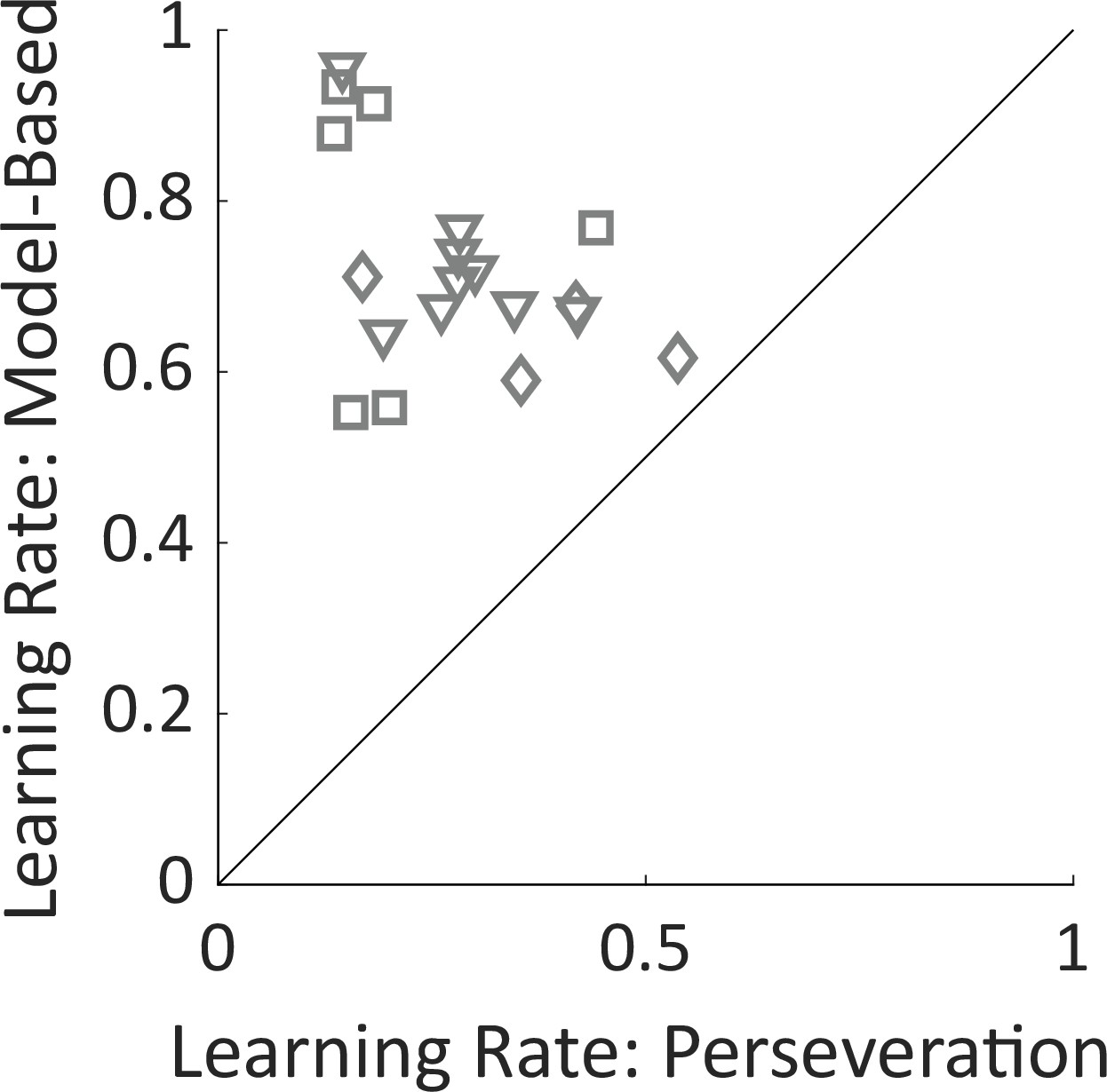
Learning rate parameters.
Fit learning rate parameters from the mixture-of-agents model for the model-based planning agent and for the perseverative agent. Learning rates for perseveration are smaller for all rats, indicating that this agent takes into account a larger number of recent trials than the model-based agent does. Shapes of symbols indicate rats participating in the electrophysiology (squares), optogenetics (triangles), or sham optogenetics (diamonds) experiments.
Figure 2—figure supplement 2
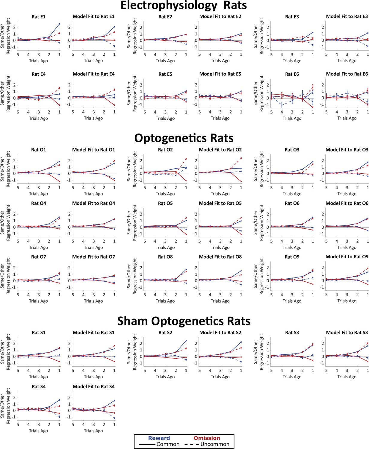
Weights of trial-history regression model, fit both to rats’ behavioral data and to synthetic datasets generated by our mixture-of-agents model fit separately to each rat.
The planning strategy is characterized by a greater tendency to repeat choices that lead to rewards following a common transition than following an uncommon transition (solid blue line above dotted blue line), as well as a greater tendency to repeat choices that lead to omissions following an uncommon transition than following a common transition (dotted red line above solid red line). All nineteen rats show evidence of such a strategy.
Figure 3 with 2 supplements
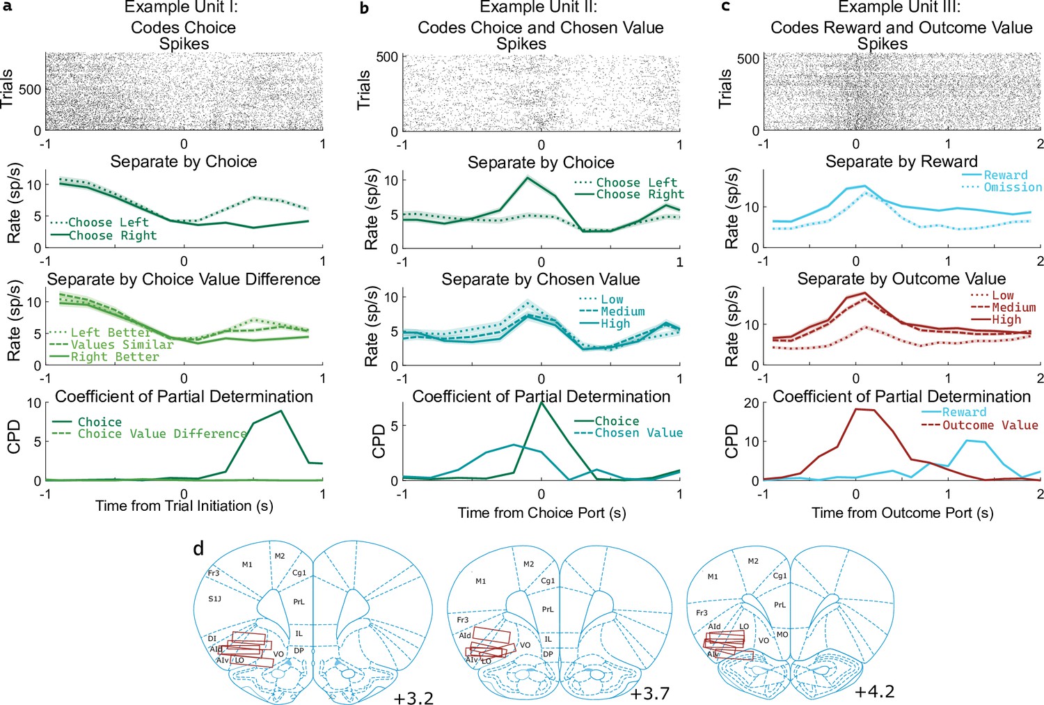
OFC units encode multiple correlated variables.
(a) Example unit whose firing rate differs both with the rat’s choice and with the difference in value between the two possible choices. An analysis using coefficient of partial determination (CPD) reveals choice coding, but no coding of expected value. (b) Example unit whose firing rate differs both with the rat’s choice and with the expected value of the choice port visited on that trial. CPD analysis reveals coding of both of these variables, though with different timecourses. (c) Example unit whose firing rate differs both with reward received and with the expected value of the outcome port visited. CPD analysis reveals coding of both of these variables, with different timecourses. (d) Approximate location of recording electrodes targeting OFC, which in rats is represented by regions LO and AIv (Paxinos and Watson, 2006; Price, 2007; Stalnaker et al., 2015), estimated using histology images (Figure 3—figure supplement 1).
Figure 3—figure supplement 1
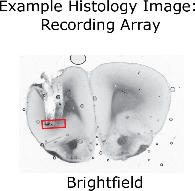
Histological verification of implant locations in OFC.
Brightfield image of a coronal section from a rat implanted with an electrode array targeting OFC. The locations of the electrode tips are visible, as is damage done when the array was removed post-mortem. Red box indicates the estimated location of electrode tips.
Figure 3—figure supplement 2
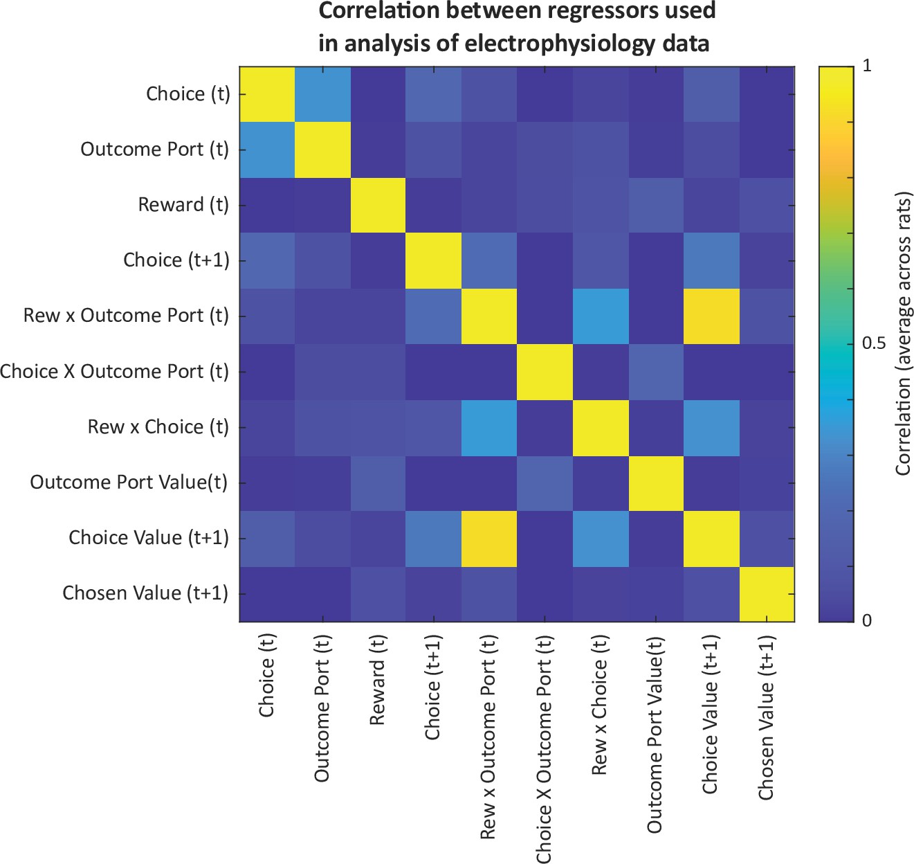
Correlations among predictors in the model used for analysis of electrophysiology data.
Correlations among regressors motivate the use of a coefficient of partial determination analysis to quantify the unique contribution of each predictor to explaining neural activity.
Figure 4 with 8 supplements
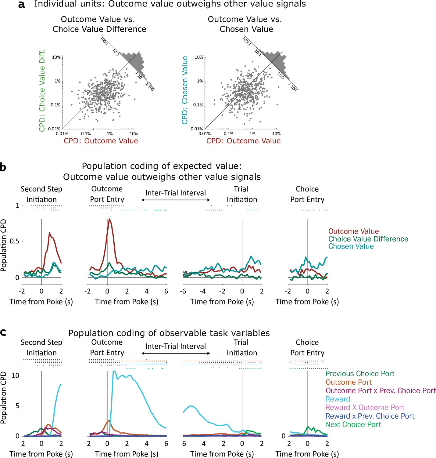
Coding of expected value of outcomes outweighs coding of expected value of choices.
(a) Left: Scatterplot showing CPD for each unit (n=477) for the outcome-value regressor against CPD for the choice-value-difference regressor, both computed in a one-second window centered on entry into the outcome port. Right: Scatterplot showing CPD for outcome-value, computed at outcome port entry, against CPD for the chosen-value regressor, computed at choice port entry. (b). Timecourse of population CPD for the three expected value regressors. We have subtracted from each CPD the mean CPD found in permuted datasets. (c) Timecourse of population CPD for the remaining regressors in the model, which reflect observable variables and interactions between them.
Figure 4—figure supplement 1
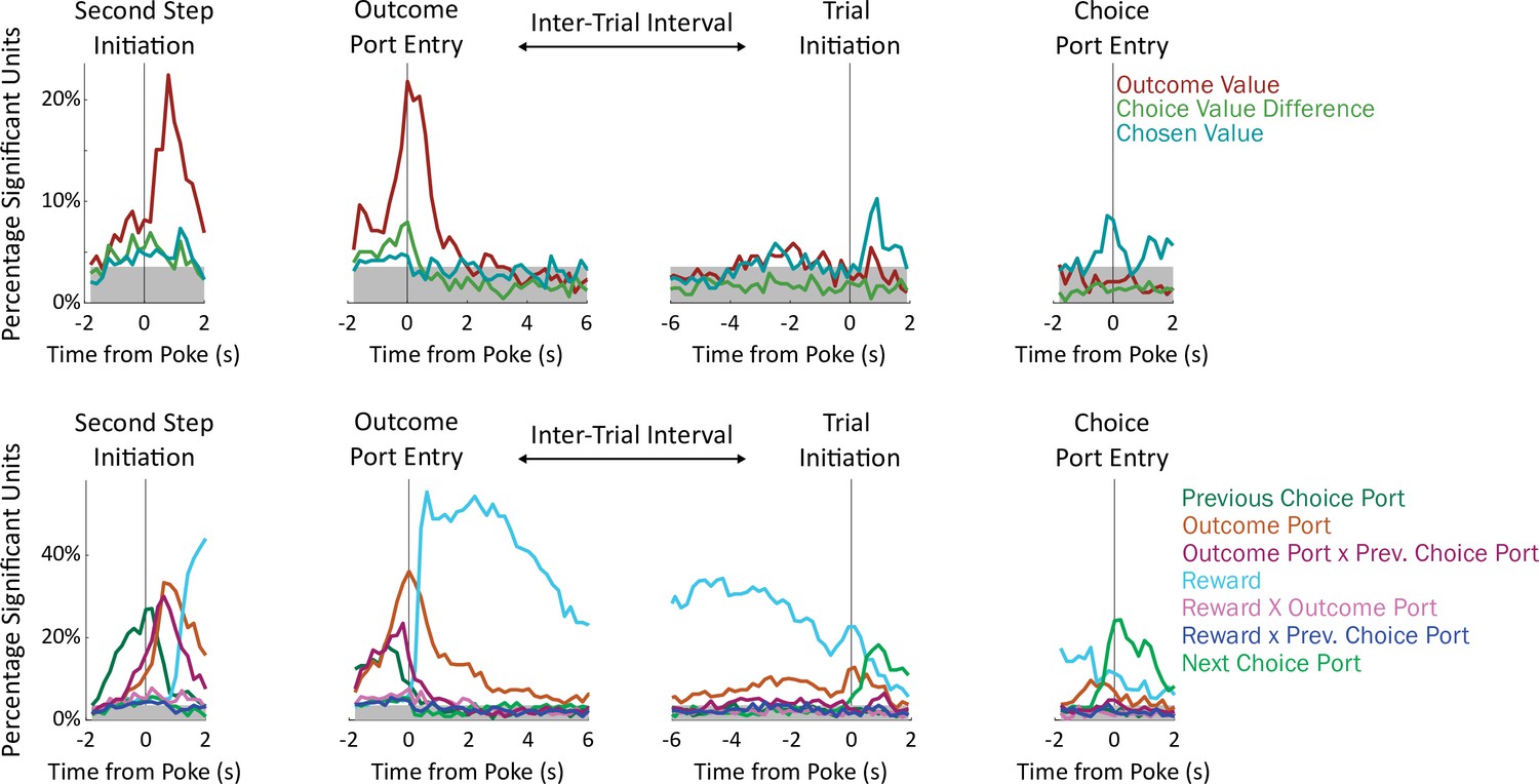
Fraction of units significantly encoding each regressor in each time bin.
Units were deemed significant if they earned a coefficient of partial determination larger than that of 99% of permuted datasets for that regressor in that time bin. Gray shading indicates a threshold for population-level significance (17/477 units; equivalent to p=2 × 10⁻⁶ by a Bernoulli test uncorrected; p<0.01 after Bonferroni correction).
Figure 4—figure supplement 2
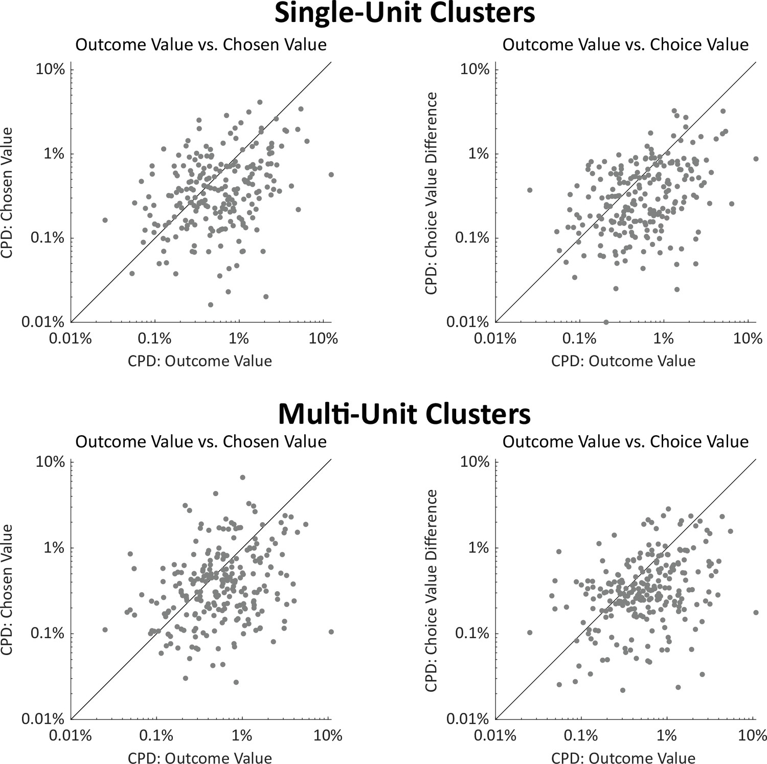
Coefficients of partial determination for value regressors, separately for single-unit and multi-unit clusters.
Above. Right: Scatterplot showing CPD for each single unit (n=251) for the outcome-value regressor against CPD for the choice-value-difference regressor, both computed in a one-second window centered on entry into the outcome port. Right: Scatterplot showing CPD for outcome-value, computed at outcome port entry, against CPD for the chosen-value regressor, computed at choice port entry. below. As above but for multi-unit clusters (n=226). In all panels, CPD for outcome value is greater than for choice-related value information (all p<10–7, signrank test. See also Figure 4a).
Figure 4—figure supplement 3
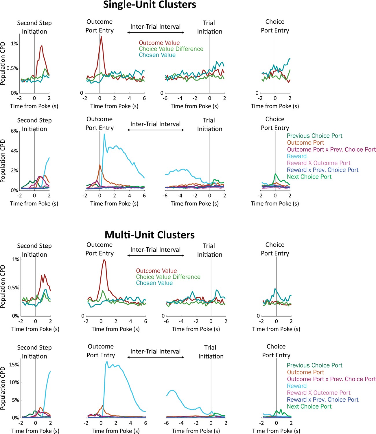
Timecourse of population CPD for the regressors in our model, considering only single-unit clusters (above) or considering only multi-unit clusters (below).
See also Figure 2a and c.
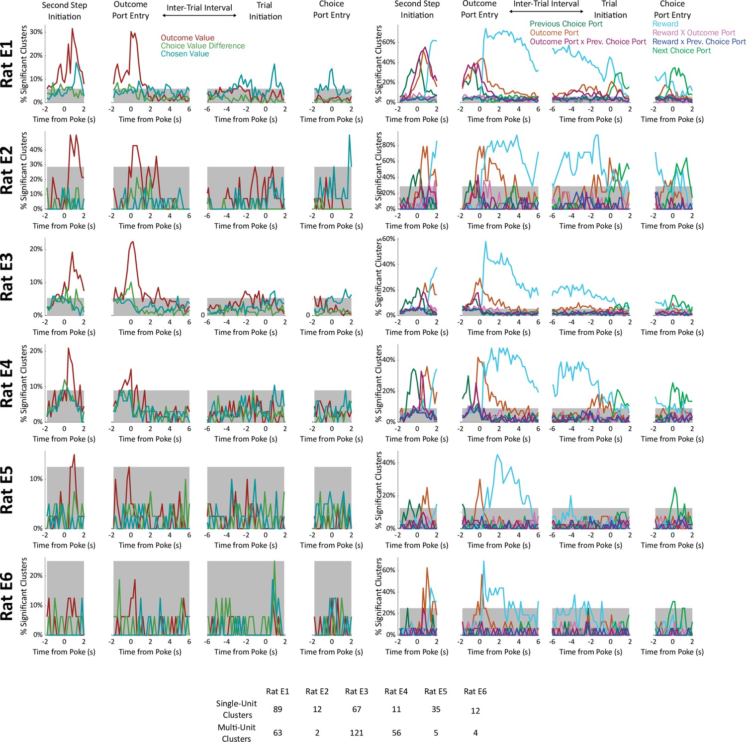
Figure 4—figure supplement 4
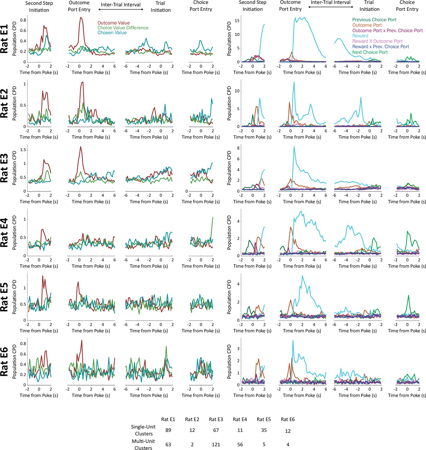
Analysis considering each rat individually.
Above: Population CPD computed separately for units from each rat in the dataset. Below: Number of single-unit and number of multi-unit clusters recorded in each rat.
Figure 4—figure supplement 5
Fraction of significant units, considering each rat individually.
Units were deemed significant if they earned a coefficient of partial determination larger than that of 99% of permuted datasets for that regressor in that time bin. Gray shading indicates a threshold for rat-level significance (p=2 × 10⁻⁶ by a Bernoulli test uncorrected; p<0.01 after Bonferroni correction).
Figure 4—figure supplement 6
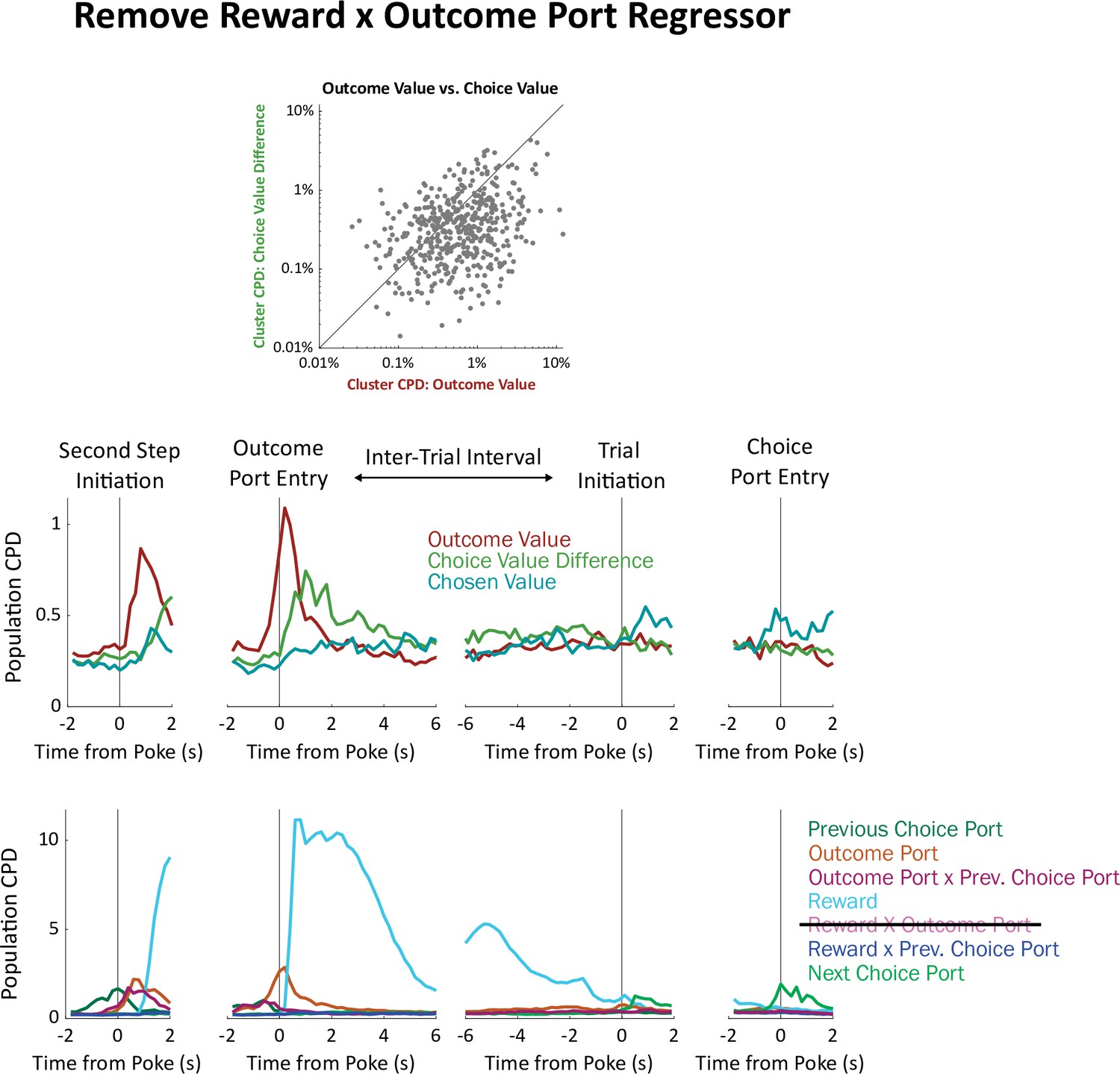
Analysis removing the outcome-by-reward interaction regressor.
The coefficient of partial determination earned by each regressor is sensitive to our choice of which other regressors to include in the model. The strength of this sensitivity depends on the correlation between the regressors (adding an orthogonal regressor will not affect CPD; adding a perfectly correlated regressor will reduce CPD to zero). The ‘choice value difference’ regressor in our model is highly correlated with one of our other regressors ‘outcome port by reward interaction’. This is because, in our model, outcome port and reward information are used to update outcome port values, which in turn update choice port values: a reward at the left outcome port or an omission at the right outcome port will increase the relative value of one choice port; a reward at the right outcome port or an omission at the left outcome port will increase the relative value of the other. This raises the possibility that our finding that the choice value difference regressor earns a relatively small CPD is an artifact of this correlation. To check this, we re-ran our regression analysis without the ‘outcome port by reward interaction’ regressor. Plots of individual clusters (a) and of the population timecourse (b) show that choice value difference still earns ambler CPDs than outcome value.
Figure 4—figure supplement 7
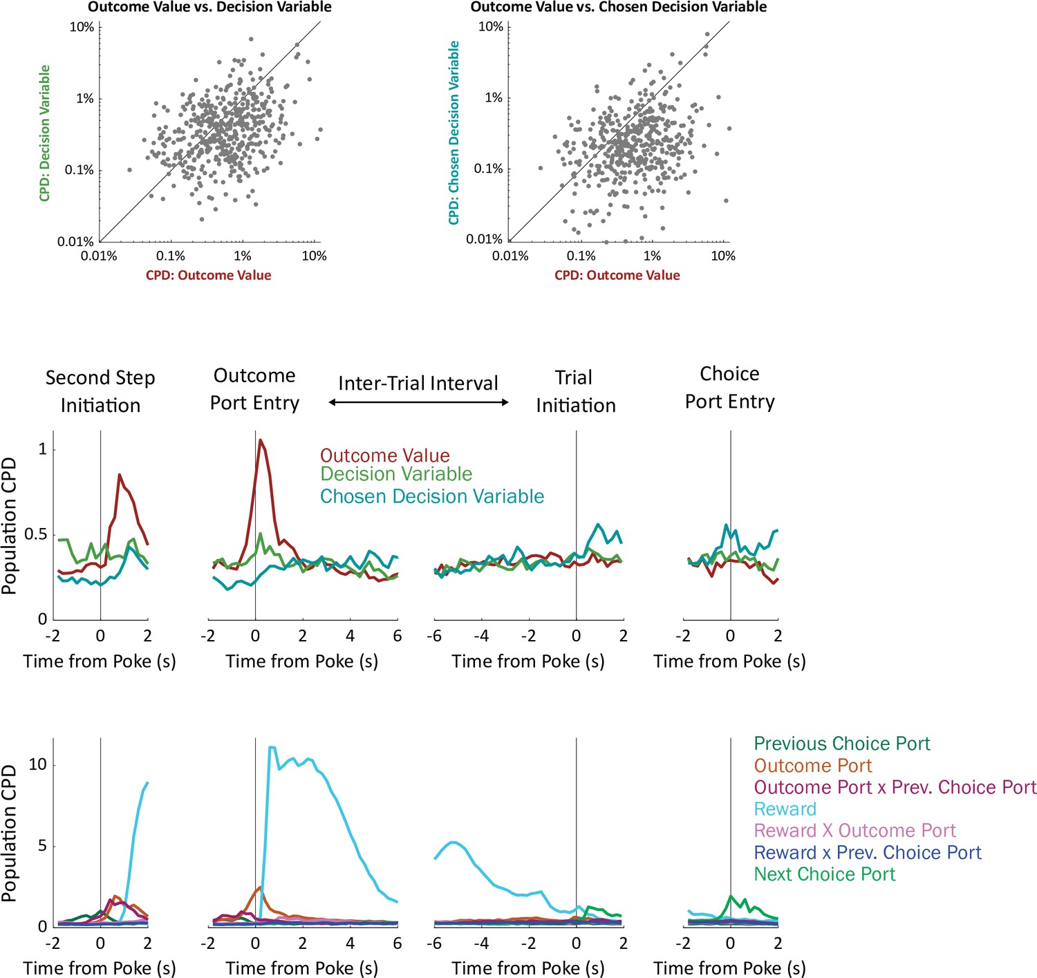
Analysis using alternative choice-related value regressors.
To compute choice-related value regressors, we used the expected values of the model-based planning component of our cognitive model (Q, see Figure 2a). However, the decision variable used by our model is not this expected value in isolation, but instead a weighted sum including expected value as well as variables related to perseveration and novelty preference (P and N, Figure 2a). Here, we compute analogs of choice value difference and of chosen value in terms of this decision variable instead of in terms of Q.
Figure 4—figure supplement 8
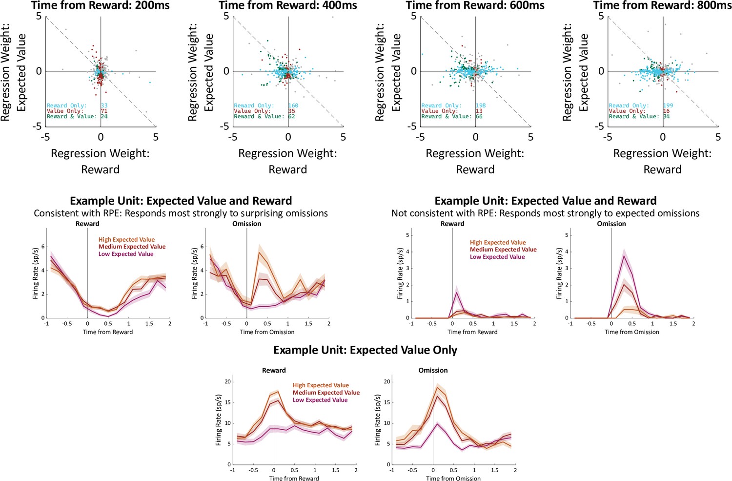
Correlates of reward prediction error.
It has been suggested that OFC causes value-guided learning in other brain regions via signaling of reward prediction errors (RPE; Banerjee et al., 2020). RPE is defined as the difference between the reward that was actually experienced and the reward that was expected. Above: We tested whether our OFC units tended to carry such a signal by examining the fit weights from our regression model in the time bins immediately following reward, following the method of Sul et al., 2010. A unit signaling RPE in our task is expected to have equal and opposite regression weights for reward and for outcome port expected value. Considering all units, we find that there is a weak but significant tendency for these weights to have opposite sign in two of the time bins (400ms: 257/477, 54%, p=0.04; 600ms: 262/477, 55%, p=0.01). Considering only units which correlate significantly with both reward and expected value, there was a similar trend (400ms: 37/62, 60%, p=0.05; 600ms: 39/66, 59%, p=0.05). These results are consistent with the idea that OFC contains units which correlate with RPE, with the caveats that it also contains a substantial number of units which correlate with its opposite (reward expected plus reward received), as well as units which correlate with expected reward without correlating with reward itself at all. Below: Example units illustrating these three patterns.
Figure 5 with 5 supplements
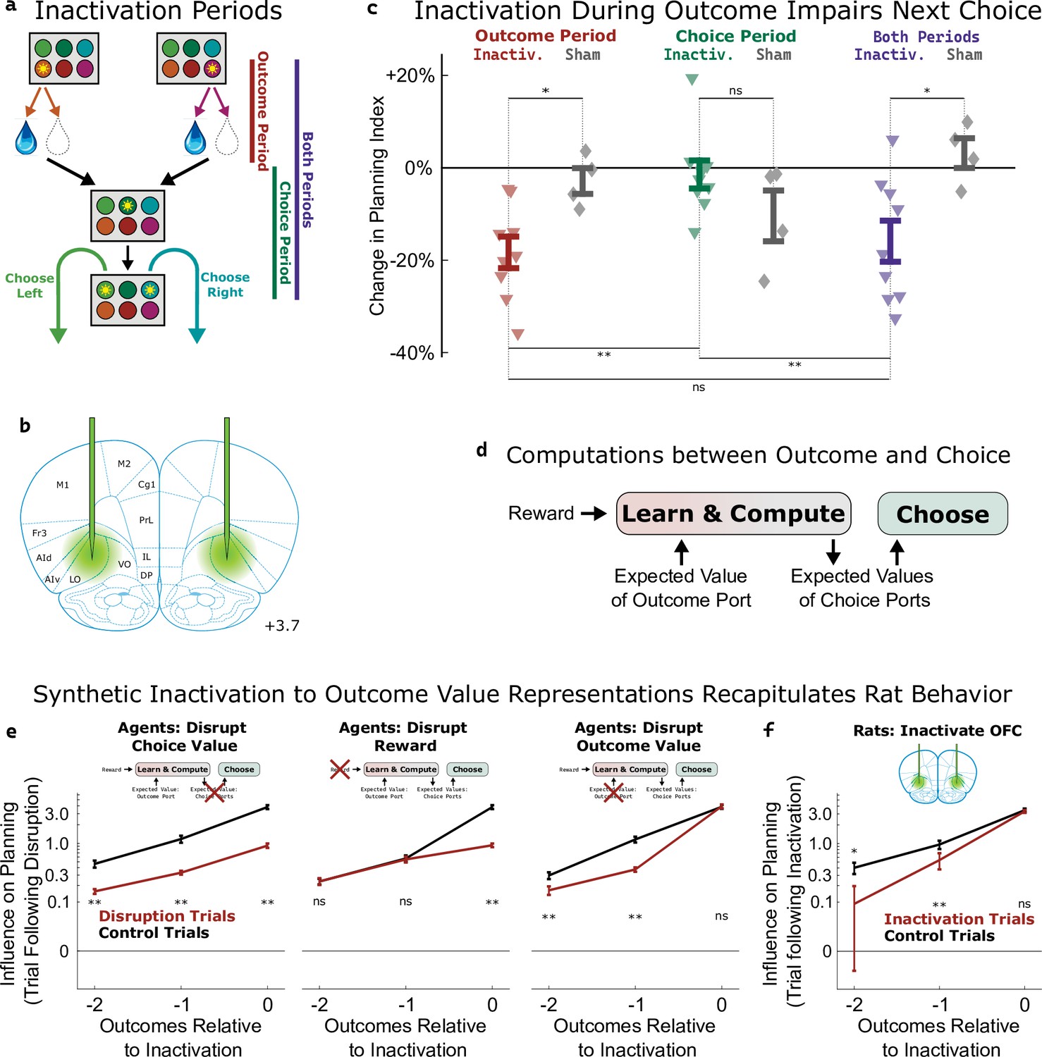
Inactivation of OFC attenuates influence of outcome values.
(a) Three time periods of inactivation. Outcome-period inactivation began when the rat entered the outcome port, and continued until the rat exited the port, or for a minimum of two seconds. Choice-period inactivation began after this outcome period, and continued until the rat entered the choice port on the next trial, or for a maximum of 15 s. Both-period inactivation encompassed both of these periods. (b) Target location for optical fiber implants. See Figure 5—figure supplement 1 for estimated actual locations in individual rats. Coronal section modified from Paxinos and Watson, 2006. (c) Effects of inactivation on the planning index on the subsequent trial for experimental rats (n=9, colored triangles) and sham-inactivation rats (n=4, gray diamonds). Bars indicate standard errors across rats. (d) Simplified schematic of the representations and computations that take place in our software agent between the delivery of the outcome on one trial and the choice on the next. Compare to Figure 2a. (e) Analysis of synthetic datasets created by disrupting different representations within the software agent on a subset of trials. Each panel shows the contribution to the planning index of trial outcomes at different lags on choices, both on control trials (black) and on trials following disruption of a representation (red). Bars indicate standard error across simulated rats (see Methods) (f) Same analysis as in c, applied to data from optogenetic inactivation of the OFC during the outcome period.
Figure 5—figure supplement 1
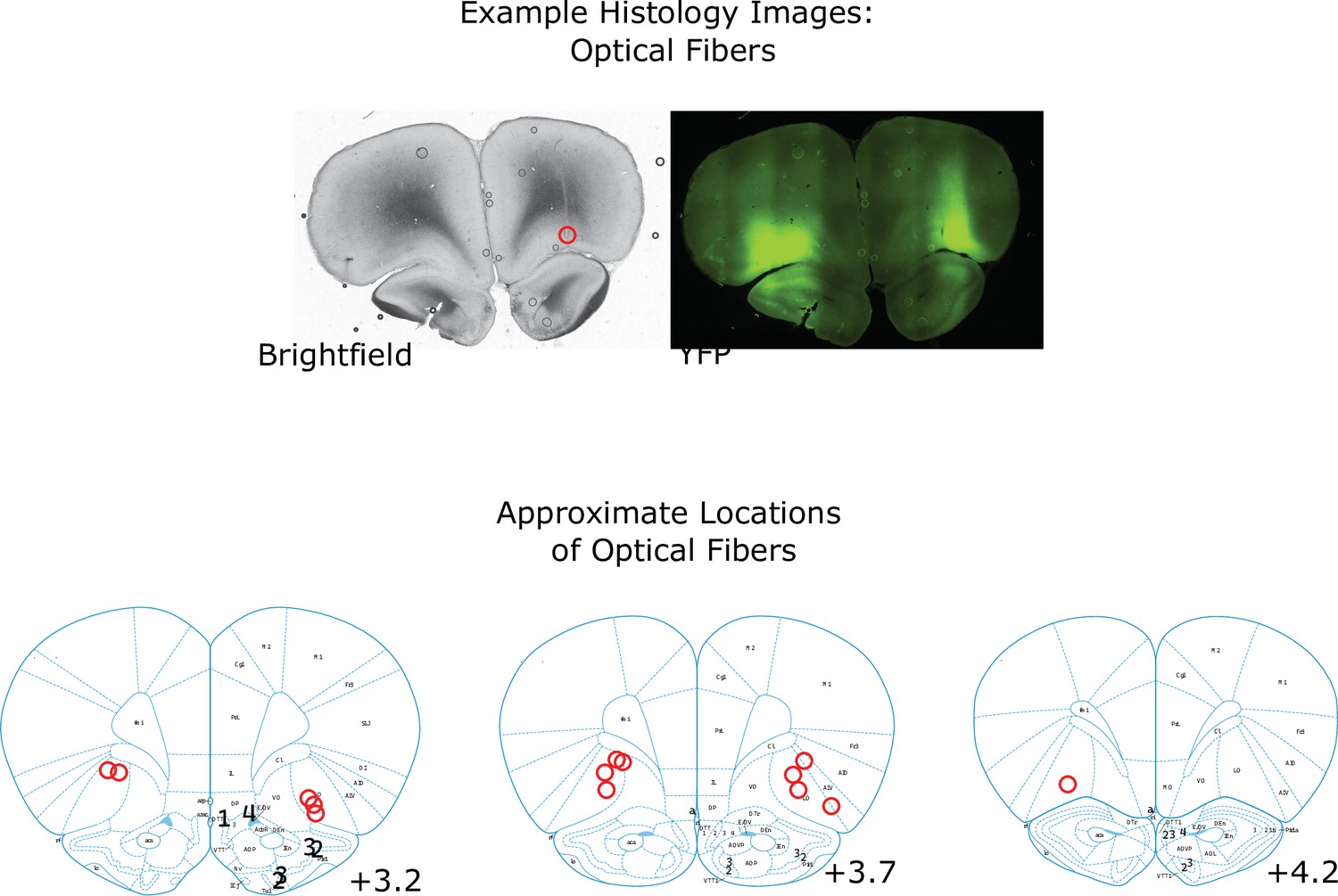
Locations of optogenetics Implants.
Example brightfield and YFP images of a coronal section taken from a rat implanted with optical fibers and infected with AAV-halorhodopsin. The location of the optical fiber on the right is visible as a scar (optical fiber on the left is visible in a different coronal section in this rat). The area of expression is visible in the YFP channel. Below: Estimates of the locations of all recording electrodes and fiber tips, obtained by comparing histology images to the reference atlas (Paxinos and Watson, 2006).
Figure 5—figure supplement 2
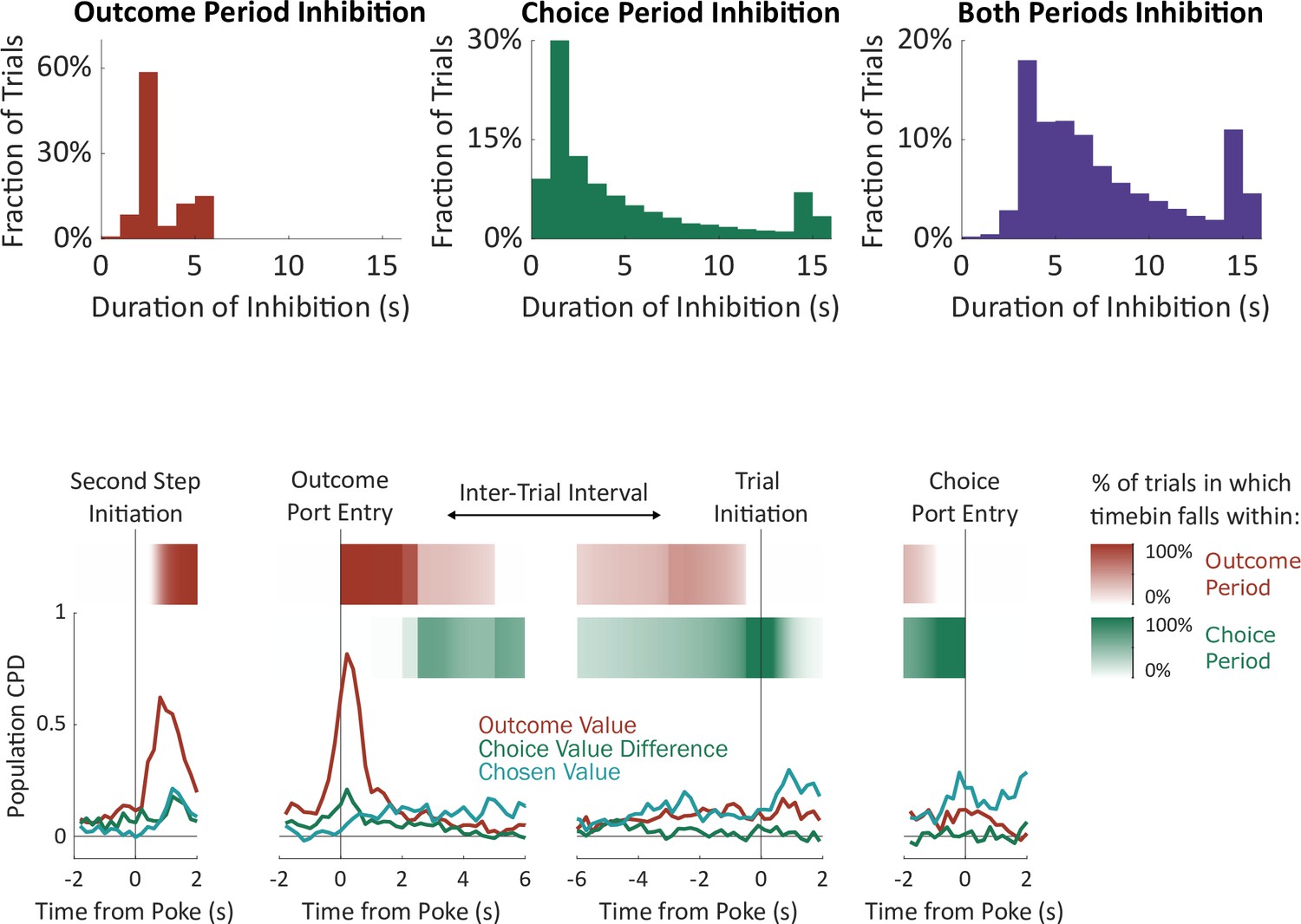
Periods of optogenetic inhibition.
The ‘outcome period’ on each trial was defined as beginning when the rat entered the outcome port, and ending either when the rat had left the outcome port for a continuous period of one second or more or after 2.5 s (unrewarded trials) or 5 s (rewarded trials). The ‘choice period’ was defined as beginning at the end of the outcome period, and ending when the rat entered the choice port on the subsequent trial. ‘Both periods’ inactivation began at entry into the outcome port and ended at entry into the choice port on the subsequent trial. For both ‘choice period’ and ‘both periods’ inactivation, an upper limit of 15 seconds was imposed. Trials on which inactivation ended due to this limit were not analyzed. Above: Histograms of the total duration of inactivation in each condition. Below: Relationship between the timebins used in electrophysiology analysis and the optogenetic inactivation periods. Line plot shows the population CPD for each of the three value-related regressors from the electrophysiology experiment (identical to Figure 4b). Red and green stripes show the probability of each timebin being in each of the optogenetic inactivation periods, computed using the optogenetics dataset.
Figure 5—figure supplement 3
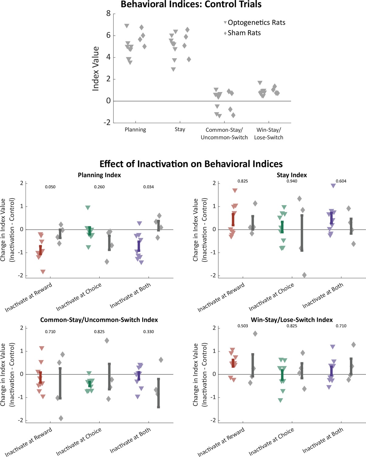
Effects of optogenetics on all behavioral indices.
Above: Regression-based behavioral indices computed considering only trials that were not preceded by inactivation, shown separately for optogenetics rats (triangles) and sham optogenetics rats (diamonds). Behavior was similar in the two groups of rats. Below: Difference in behavioral indices between trials that were preceded by inactivation in each time period and those that were not preceded by inactivation. Only for the planning index were there significant differences between optogenetics and sham optogenetics rats (p-values shown from two-sample rank sum test).
Figure 5—figure supplement 4
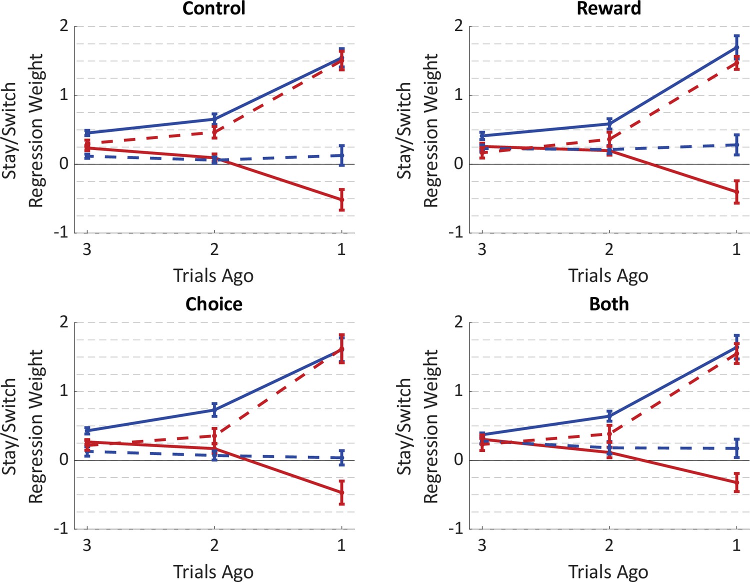
Average fit weights of the trial-history regression model to behavioral data from the optogenetics experiment.
Weights were estimated separately for trials preceded by (a) no inhibition, (b) inhibition during the reward period, (c) inhibition during the choice period, or (d) inhibition during both periods. Weights for individual rats are shown in Figure 5—figure supplement 5.
Figure 5—figure supplement 5
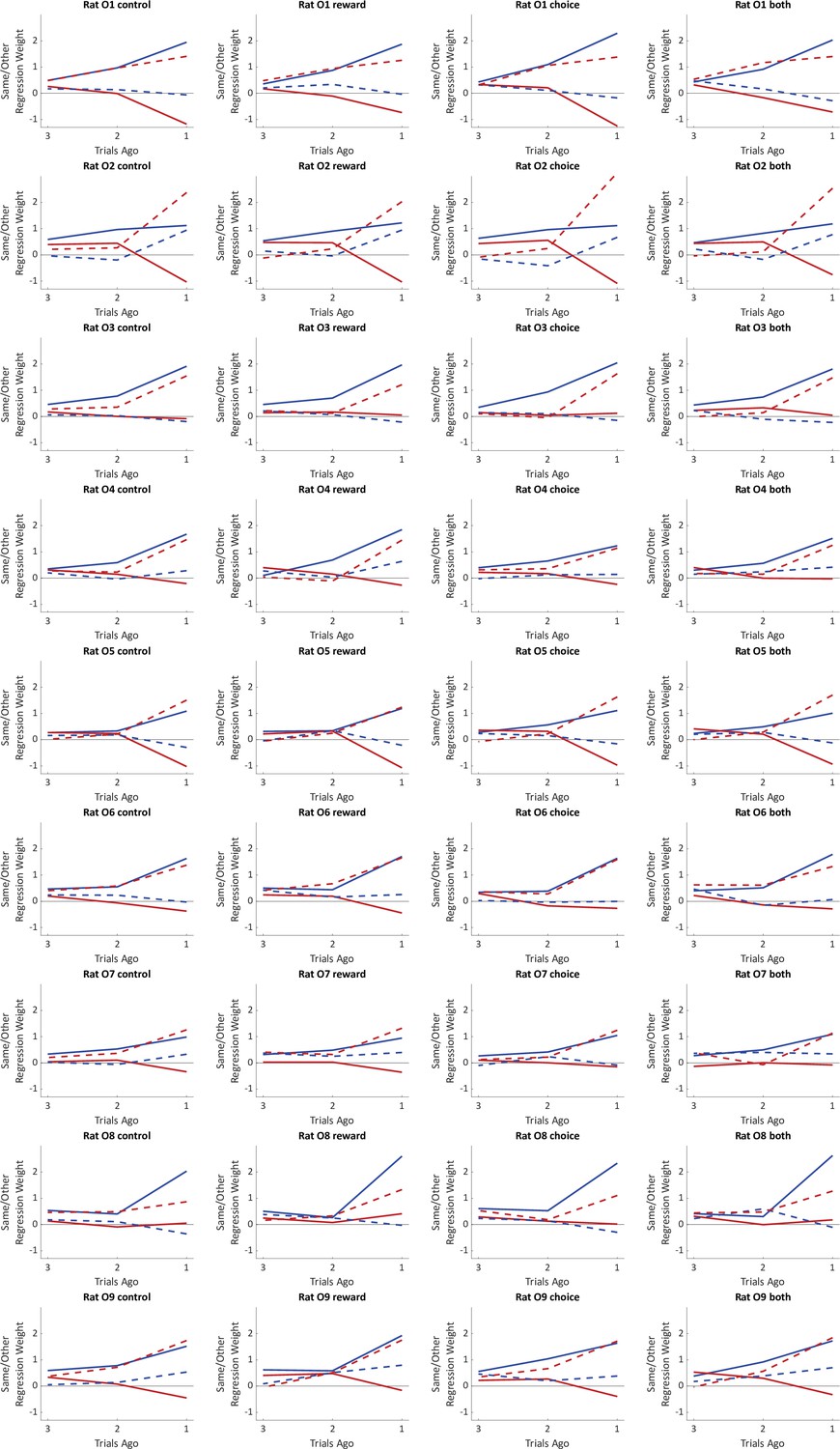
Fit weights of the trial history regression model for individual rats in the optogenetics experiment.
Weights were estimated separately for trials preceded by no inhibition, inhibition during the reward period, inhibition during the choice period, or inhibition during both periods.
Additional files
Download links
A two-part list of links to download the article, or parts of the article, in various formats.
Downloads (link to download the article as PDF)
Open citations (links to open the citations from this article in various online reference manager services)
Cite this article (links to download the citations from this article in formats compatible with various reference manager tools)
Value representations in the rodent orbitofrontal cortex drive learning, not choice
eLife 11:e64575.
https://doi.org/10.7554/eLife.64575


