DIPPER, a spatiotemporal proteomics atlas of human intervertebral discs for exploring ageing and degeneration dynamics
- School of Biomedical Sciences,, Hong Kong
- The University of Hong Kong Shenzhen of Research Institute and Innovation (HKU-SIRI), China
- Centre for Blood Research, Faculty of Dentistry, University of British Columbia, Canada
- Proteomics and Metabolomics Core Facility, Hong Kong
- Department of Orthopaedics Surgery and Traumatology, HKU-Shenzhen Hospital, China
- Department of Surgery, McGill University, Canada
- Centre for PanorOmic Sciences (CPOS), Hong Kong
Figures
Figure 1 with 4 supplements

Outline of samples, workflow, MRI, and global overview of data in DIPPER.
(A) Schematic diagram showing the structure of the samples, data types, and flow of analyses in DIPPER. is the number of individuals. is the number of genome-wide profiles. (B) Clinical T2-weighted MRI images (3T) of the young lumbar discs in the sagittal and transverse plane (left and right panels), T1 MRI image of the young lumbar spine (middle panel). (C) High-resolution (7T) T2-weighted MRI of the aged lower lumbar spine in sagittal (left panel) and transverse plane (right panel). (D) Diagram showing the anatomy of the IVD and locations where the samples were taken. VB: vertebral body; NP, nucleus pulposus; AF, annulus fibrosus; IAF: inner AF; OAF: outer AF; NP/IAF: a transition zone between NP and IAF. (E) Venn diagrams showing the overlaps of detected proteins in the four major compartments. Top panel, young and aged profiles; middle, young only; bottom, aged only. (F) Barchart showing the numbers of proteins detected per sample, categorised into matrisome (coloured) or non-matrisome proteins (grey). (G) Barcharts showing the composition of the matrisome and matrisome-associated proteins. Heights of bars indicate the number of proteins in each category expressed per sample. The N number in brackets indicate the aggregate number of proteins. (H) Violin plots showing the level of subcategories of ECMs in different compartments of the disc. The green number on top of each violin shows its median. LFQ: label-free quantification. (I) Top 30 HGNC gene families for all non-matrisome proteins detected in the dataset. (J) Violin plots showing the averaged expression levels of 10 detected histones across the disc compartments and age-groups. (K) Scatter-plot showing the co-linearity between GAPDH and histones.
Figure 1—figure supplement 1
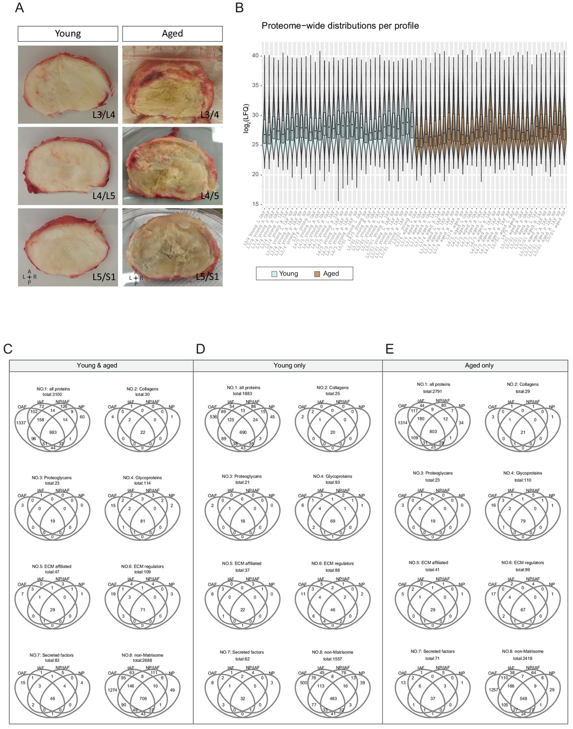
Gross images of the discs and overview of the static spatial proteomic data.
(A) Gross images of the young and aged cadaveric discs. (B) Proteome-wide distributions per profile across all 66 profiles of the static spatial proteome data. The profiles were named with levels, ages, directions, and compartments. (C)-(E) Venn diagrams of detected proteins among the four major IVD compartments (OAF, IAF, NP/IAF, and NP), per age-group, and per protein category.
Figure 1—figure supplement 2
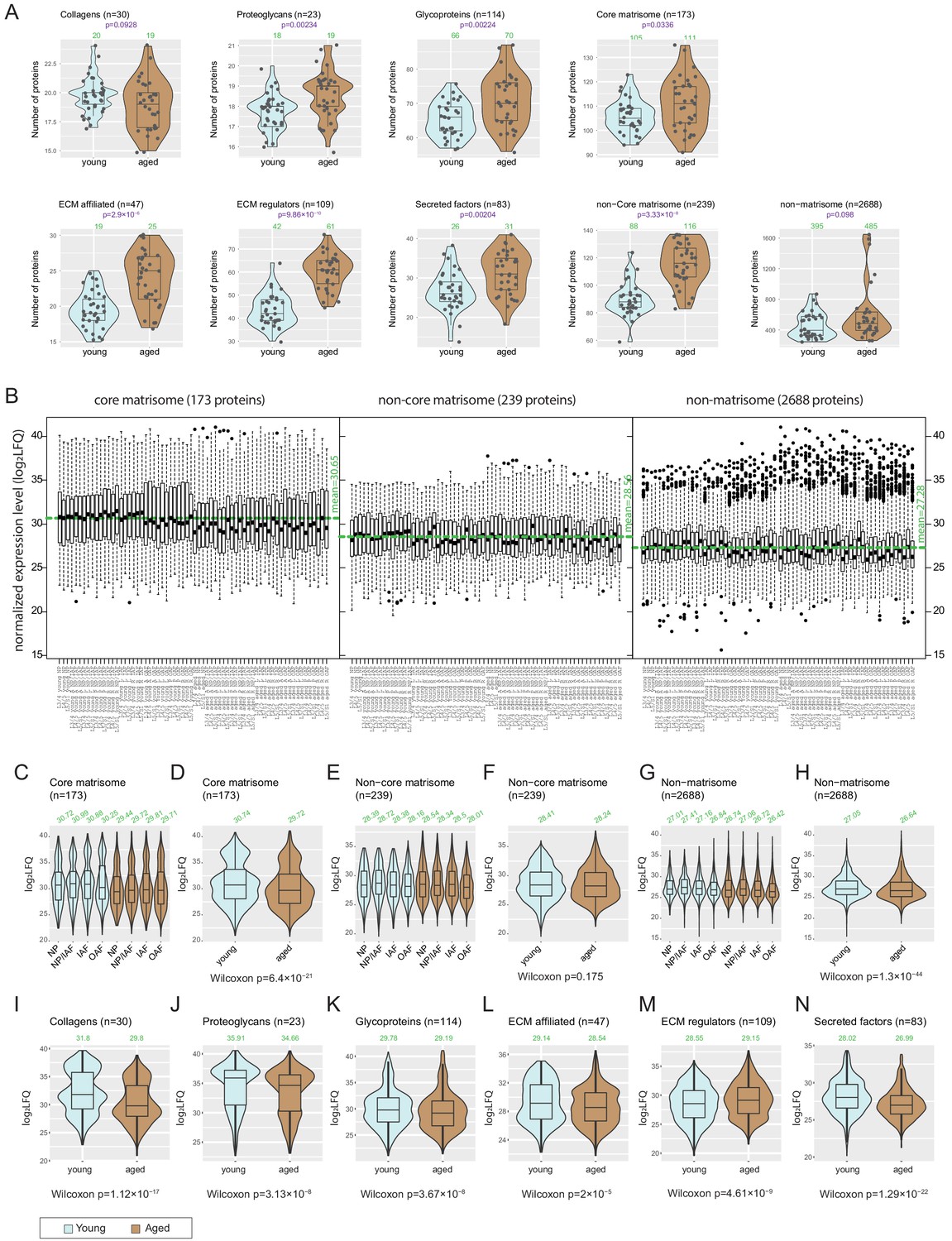
Numbers of proteins detected and protein levels for each combination of sample groups.
(A) Violin-plots showing numbers of proteins detected per age-group, for all categories of extracellular matrix (ECM) and non-ECM proteins. The green numbers on top of each violin show the median number of proteins detected per respective sample group. (B) Box-plots showing the expression levels of core-matrisome, non-core matrisome, and non-matrisome proteins. Horizontal green line indicates average. (C-H) Violin plots showing the expression levels of major ECM categories across compartments and age-groups. (I-N) Violin plots showing the expression levels of subcategories of ECM proteins across age-groups. The green numbers on top of each violin show the median number of proteins detected per respective sample group.
Figure 1—figure supplement 3

Heatmaps showing different categories of detected proteins.
(A-C) Profiles and their hierarchical clustering patterns of all detected transcription factors or DNA-binding proteins (A), cell surface markers (B), inflammatory proteins (C). (D) Numbers of signalling proteins detected per compartment and age-group in the data. The colour scale corresponds to proteins in overlap within each entry divided by total number of proteins in the pathway.
Figure 1—figure supplement 4
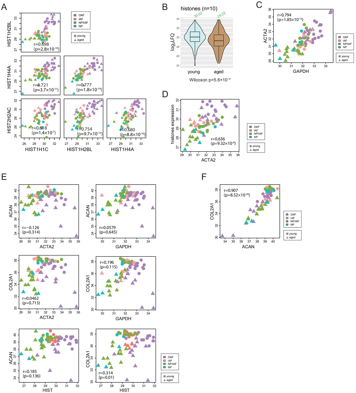
Histones and housekeeping genes reflect cellularities.
(A) Scatter-plots showing the co-expression of four histone proteins that were detected in over 60 profiles. (B) Violin plot showing the expression levels of the histones across age-groups. (C) Scatter plot showing the co-expression between ACTA2 and the average of histones. (D) Scatter plot showing the co-expression between ACTA2 and GAPDH. (E) Scatter plots showing the co-expression between ACTA2, GAPDH, and histones, and COL2A1, and ACAN. (F) Scatter plot showing the co-expression between COL2A1 and ACAN. All values are in log2(LFQ). r is Pearson correlation coefficient.
Figure 2 with 1 supplement
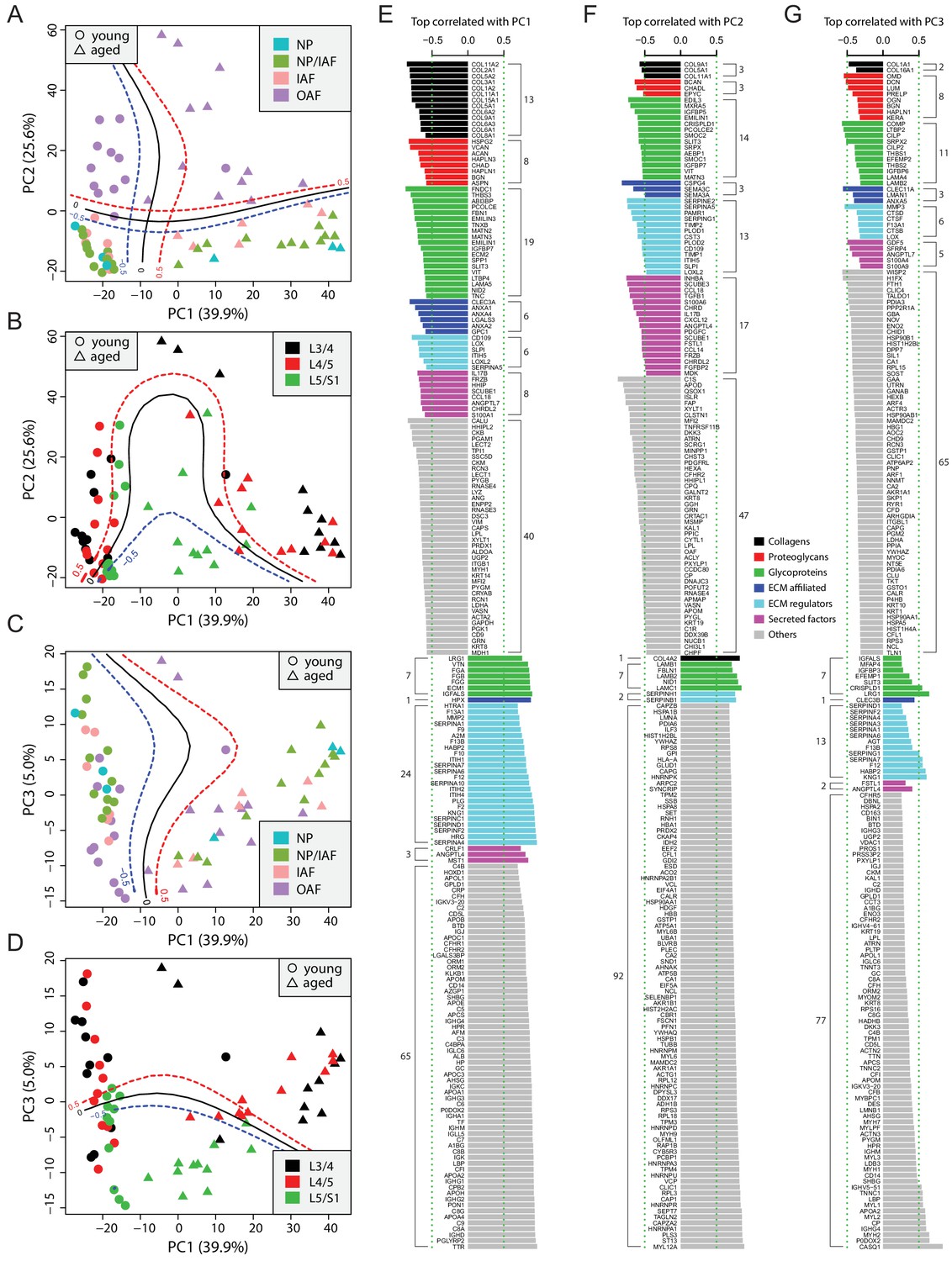
Principle component analysis (PCA) of the 66 static spatial profiles based on a set of 507 genes selected by optimal cutoff (see Figure 2—figure supplement 1A–C).
(A) Scatter-plot of PC1 and PC2 colour-coded by compartments, and dot-shaped by age-groups. Solid curves are the support vector machines (SVMs) decision boundaries between inner disc regions (NP, NP/IAF, IAF) and OAF, and dashed curves are soft boundaries for probability equal to ±0.5 and are applied to all plots in this figure. (B) Scatter-plot of PC1 and PC2 colour-coded by disc levels. The SVM boundaries are trained between L5/S1 and upper levels (L3/4 and L4/5). (C) Scatter-plot of PC1 and PC3, colour-coded by disc compartments. The SVM boundaries are trained between inner disc regions and OAF. (D) Scatter-plot of PC1 and PC3, colour-coded by disc levels. The SVM boundaries are trained between L5/S1 and upper levels (L3/4 and L4/5). (E) Top 100 positively and negatively correlated genes with PC1, colour-coded by ECM categories. (F) Top 100 positively and negatively correlated genes with PC2, colour-coded by extracellular matrix (ECM) categories. (G) Top 100 positively and negatively correlated genes with PC3, colour-coded by ECM categories.
Figure 2—figure supplement 1
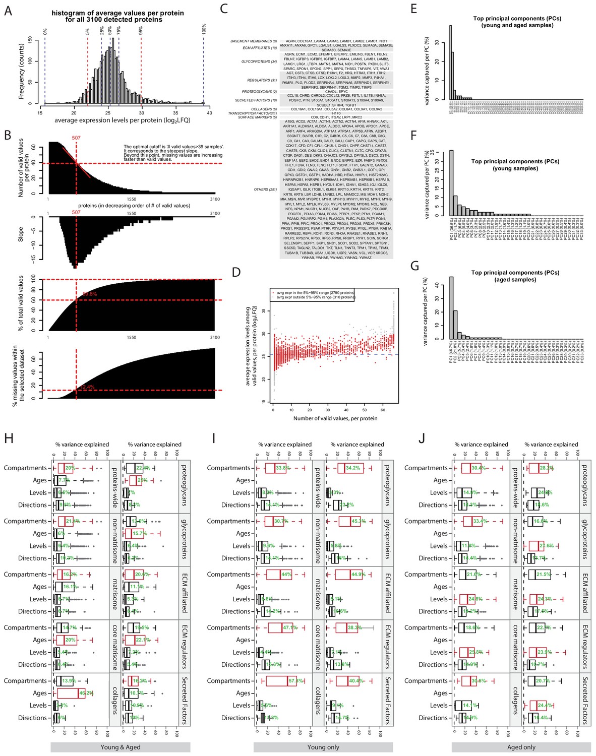
Selection of genes for performing principle component analysis (PCA) and results of ANOVA on assessing global data variability.
(A) Histogram and key percentiles of the average expression levels of all 3100 detected proteins. Average was calculated based on the valid samples of each protein. (B) Selecting an optimal cutoff above which proteins will be used for performing PCA. Upper panel, proteins were ordered in decreasing order by its number of valid values. Second panel: the slope of the upper panel. Third panel: the fraction of all valid values in the whole data-set captured per each cutoff. An optimal cutoff corresponding to the cutoff of ‘>39 valid values’ was found where the slope is steepest. Lower panel: the fraction of missing values within the selected dataset at each cutoff. (C) A list of the proteins (categorised by their functional families) that both meet the criteria in (B) and fall in the 5–95% range in (A). (D) A scatter plot showing the positive relation between number of valid values per protein, and the average expression level per protein. (E)-(G), the percentages of variance captured by the top principal components (PCs) in the whole dataset (E), young samples only (F), and aged samples only (G). (H)-(J) Horizontal box plots showing the percentages of variance explained by four phenotypic factors, for different scopes of protein sets. (H) Young and aged combined. (I) Young only. (J) Aged only.
Figure 3 with 3 supplements
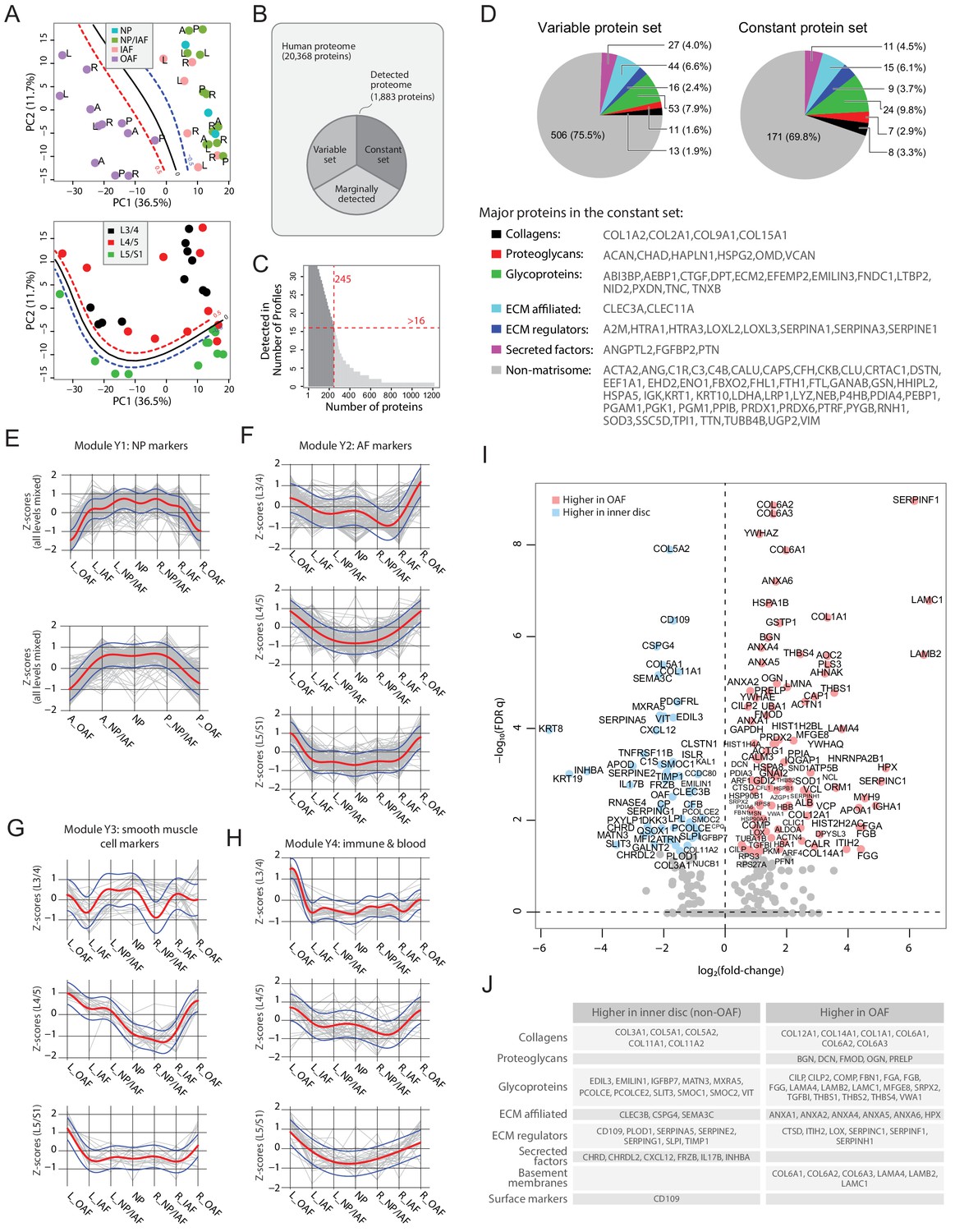
Delineating the young non-degenerated cadaveric discs’ static spatial proteome.
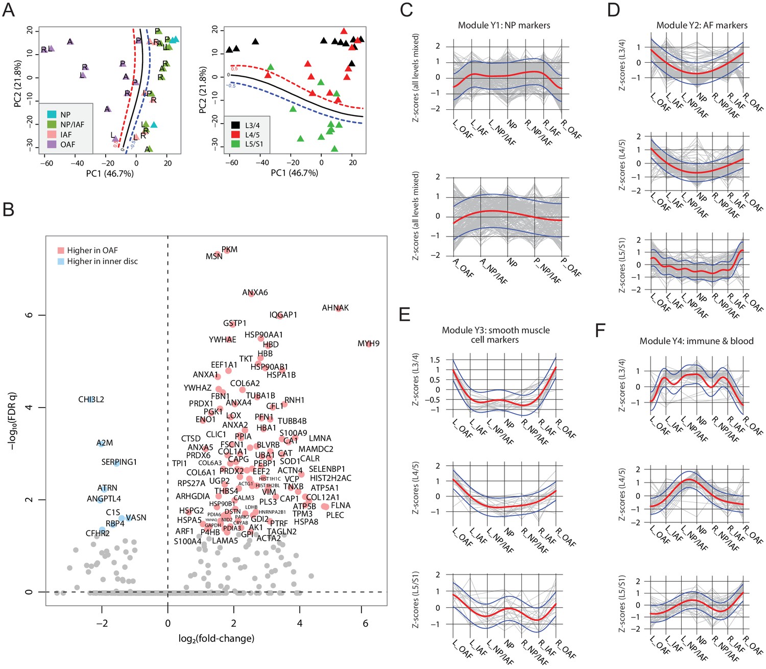
(A) Principal component analysis (PCA) plot of all 33 young profiles. Curves in the upper panel show the support vector machine (SVM) boundaries between the OAF and inner disc regions, those in the lower panel separate the L5/S1 disc from the upper disc levels. L, left; R, right; A, anterior; P, posterior. (B) A schematic illustrating the partitioning of the detected human disc proteome into variable and constant sets. (C) A histogram showing the distribution of non-DEPs in terms of their detected frequencies in the young discs. Only 245 non-DEP proteins were detected in over 16 profiles, which is thus defined to be the constant set; while the remaining ~1,000 proteins were considered marginally detected. (D) Piecharts showing the extracellular matrix (ECM) compositions in the variable (left) and constant (right) sets. The constant set proteins that were detected in all 33 young profiles are listed at the bottom. (E) Normalised expression (Z-scores) of proteins in the young module Y1 (NP signature) laterally (top panel) and anteroposterially (bottom panel), for all three disc levels combined. The red curve is the Gaussian Process Estimation (GPE) trendline, and the blue curves are one standard deviation above or below the trendline. (F) Lateral trends of module Y2 (AF signature) for each of the three disc levels. (G) Lateral trends of module Y3 (Smooth muscle cell signature) for each of the three disc levels. (H) Lateral trends of module Y4 (Immune and blood) for each of the three disc levels. (I) Volcano plot of differentially expressed proteins (DEPs) between OAF and inner disc (an aggregate of NP, NP/IAF, IAF), with coloured dots representing DEPs. (J) A functional categorisation of the DEPs in (I).
Figure 3—figure supplement 1

Additional comparisons within the young samples.
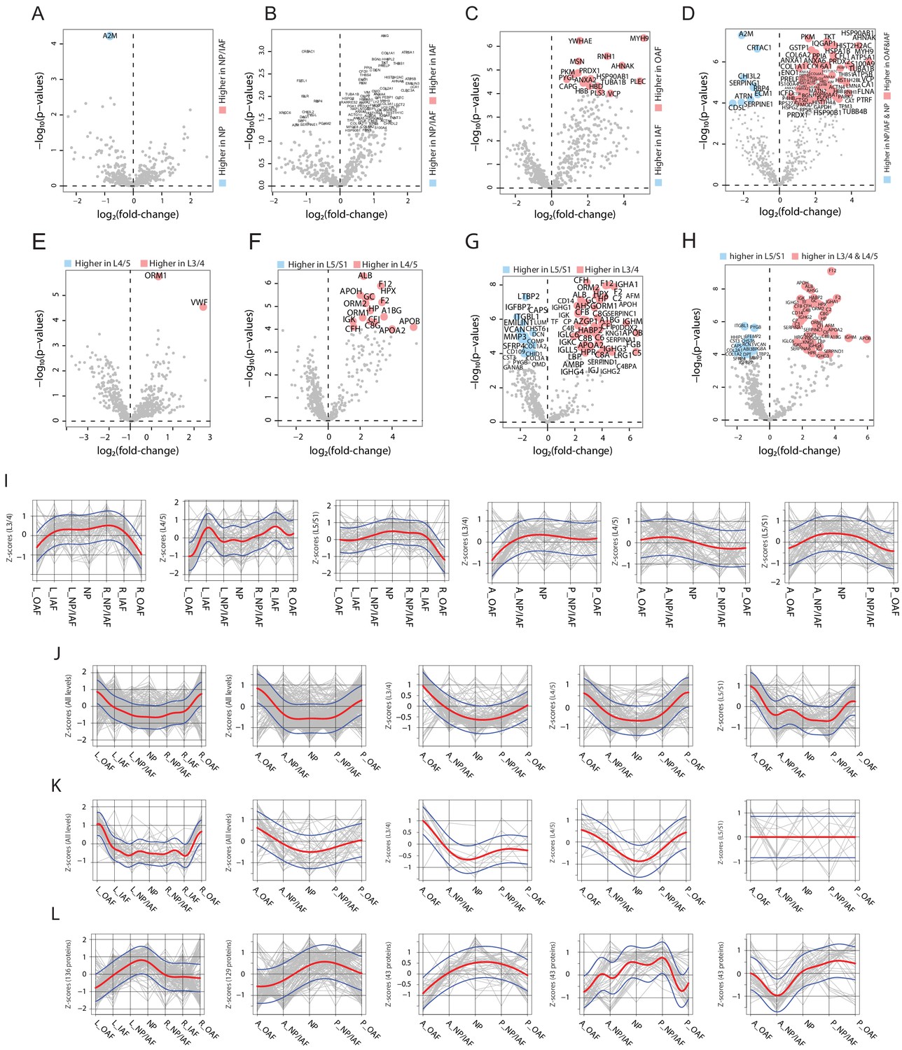
(A) Schematic diagrams showing the comparisons between different groups of samples. (B)-(U), volcano plots showing the differentially expressed proteins for each comparison listed in (A). (V–W) Dendrograms showing the clustering patterns of four samples corresponding to left (L), right (R), anterior (A), and posterior (P) directions, in OAF (V) and NP/IAF (W), respectively.
Figure 3—figure supplement 2
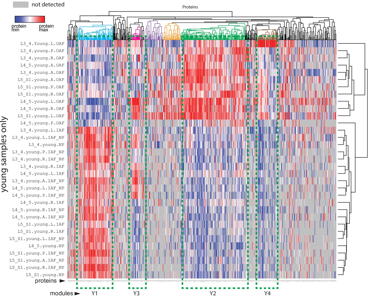
Heatmap of differentially expressed proteins (DEPs) and protein modules.
A profile-protein bi-clustering heatmap of 671 DEPs identified in 20 two-group comparisons within the young samples. For each of the comparisons, a DEP could come from three sources: statistical comparisons, fold-changes, or exclusive expressions in one group only (Materials and methods). Four protein modules were identified: Y1~Y4.
Figure 3—figure supplement 3
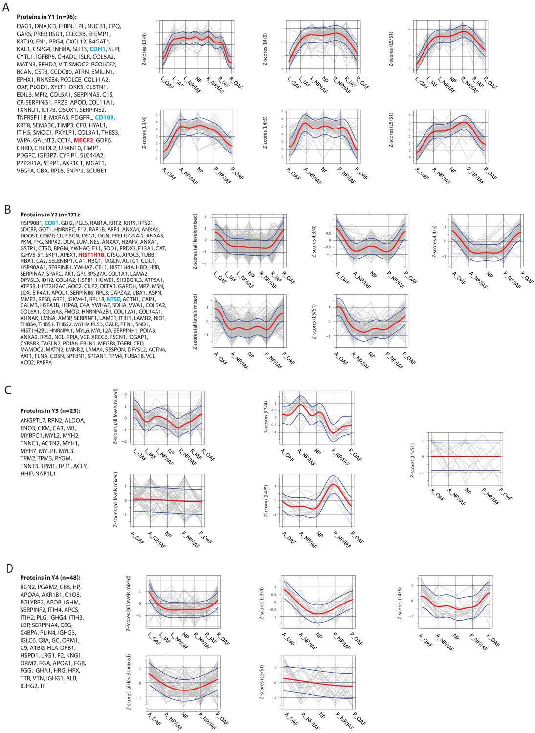
Modular trends along the lateral or anteroposterior axes in the young non-degenerated discs.
(A)-(D) Proteins in modules Y1 (A), Y2 (B), Y3 (C), and Y4 (D), and their directional trends, in the young profiles. The red curve is the Gaussian Process Estimation (GPE) trend line, and the blue curves are one standard deviation above or below the trend line. Genes in red are transcription factors or DNA-binding proteins. Genes in blue are surface markers.
Figure 4 with 1 supplement
Characterisation of the aged cadaveric discs’ static spatial proteome.
(A) Principal component analysis (PCA) plot of all the aged profiles on PC1 and PC2, colour-coded by compartments. Curves in the left panel show the support vector machine (SVM) boundaries between OAF and inner disc; those in the right panel separate the L5/S1 disc from the upper disc levels. Letters on dots indicate directions: L, left; R, right; A, anterior; P, posterior. (B) Volcano plot showing the differentially expressed proteins (DEPs) between the OAF and inner disc (an aggregate of NP, NP/IAF, and IAF), with the coloured dots representing statistically significant (FDR < 0.05) DEPs. (C) Using the same four modules identified in young samples, we determined the trend for these in the aged samples. Locational trends of module Y1 showing higher expression in the inner disc, albeit they are more flattened than in the young disc samples. Top panel shows left to right direction and bottom panel shows anterior to posterior direction. The red curve is the Gaussian Process Estimation (GPE) trendline, and the blue curves are one standard deviation above or below the trendline. This also applies to (D), (E), and (F). (D) Lateral trends for module Y2 in the aged discs. (E) Lateral trends for module Y3 in the aged discs. (F) Lateral trends for module Y4 in the aged discs.
Figure 4—figure supplement 1
Differentially expressed proteins (DEPs) between different compartments or levels and spatial trends of protein modules in the aged discs.
(A)-(H) Volcano plots showing the DEPs between different compartments or levels in the aged discs. (A) Volcano plot of DEPs between NP and NP/IAF. (B) Volcano plot of DEPs between NP/IAF and IAF. (C) Volcano plot of DEPs between IAF and OAF. (D) Volcano plot of DEPs between {NP + NP/IAF} and {IAF + OAF}. (E) Volcano plot of DEPs between L4/5 and L3/4. (F) Volcano plot of DEPs between L5/S1 and L4/5. (G) Volcano plot of DEPs between L5/S1 and L3/4. (H) Volcano plot of DEPs between lower level (L5/S1) and upper two levels combined, in the aged discs. (I)-(L), the lateral and anteroposterior trends of the four protein modules identified in (Figure 3—figure supplement 3) in the aged discs. (I) Module Y1. (J) Module Y2. (K) Module Y3. (L) Module Y4. The red curve is the Gaussian Process Estimation (GPE) trend line, and the blue curves are one standard deviation above or below the trend line.
Figure 5 with 1 supplement
Comparisons between young and aged static spatial proteomes.
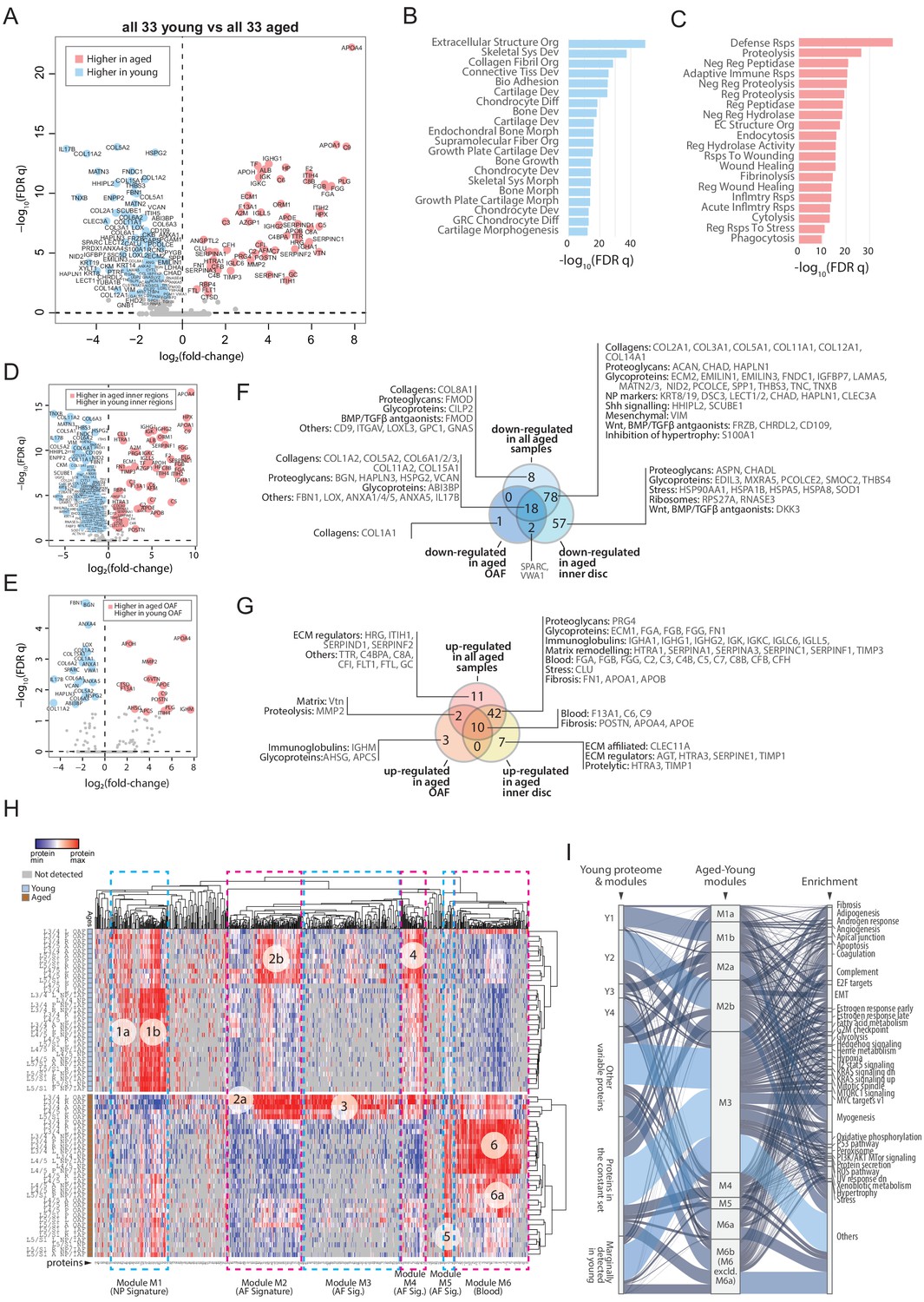
(A) Volcano plot showing the differentially expressed proteins (DEPs) between all the 33 young and 33 aged profiles. Coloured dots represent statistically significant DEPs. (B) Gene ontology (GO) term enrichment of DEPs higher in young profiles. (C) GO term enrichment of DEPs higher in aged profiles. Full names of GO terms in (B and C) are listed in Supplementary file 5. (D) Volcano plot showing DEPs between aged and young inner disc regions. (E) Volcano plot showing DEPs between aged and young OAF. (F) Venn diagram showing the partitioning of the young/aged DEPs that were downregulated in aged discs, into contributions from inner disc regions and OAF. (G) Venn diagram showing the partitioning of the young/aged DEPs that were upregulated in aged discs, into contributions from inner disc regions and OAF. (H) A heat map showing proteins expressed in all young and aged disc, with the identification of 6 modules (module 1: higher expression in young inner disc regions, modules 2 and 4: higher expression in young OAF, module 3: highly expressing in aged OAF, module 5: higher expression across all aged samples, and module 6: higher expression in aged inner disc, and some OAF). (I) An alluvial chart showing the six modules identified in (H) and their connections to the previously identified four modules and constant set in the young reference proteome; as well as their connections to enriched GO terms.
Figure 5—figure supplement 1
Comparisons of young and aged proteomes.
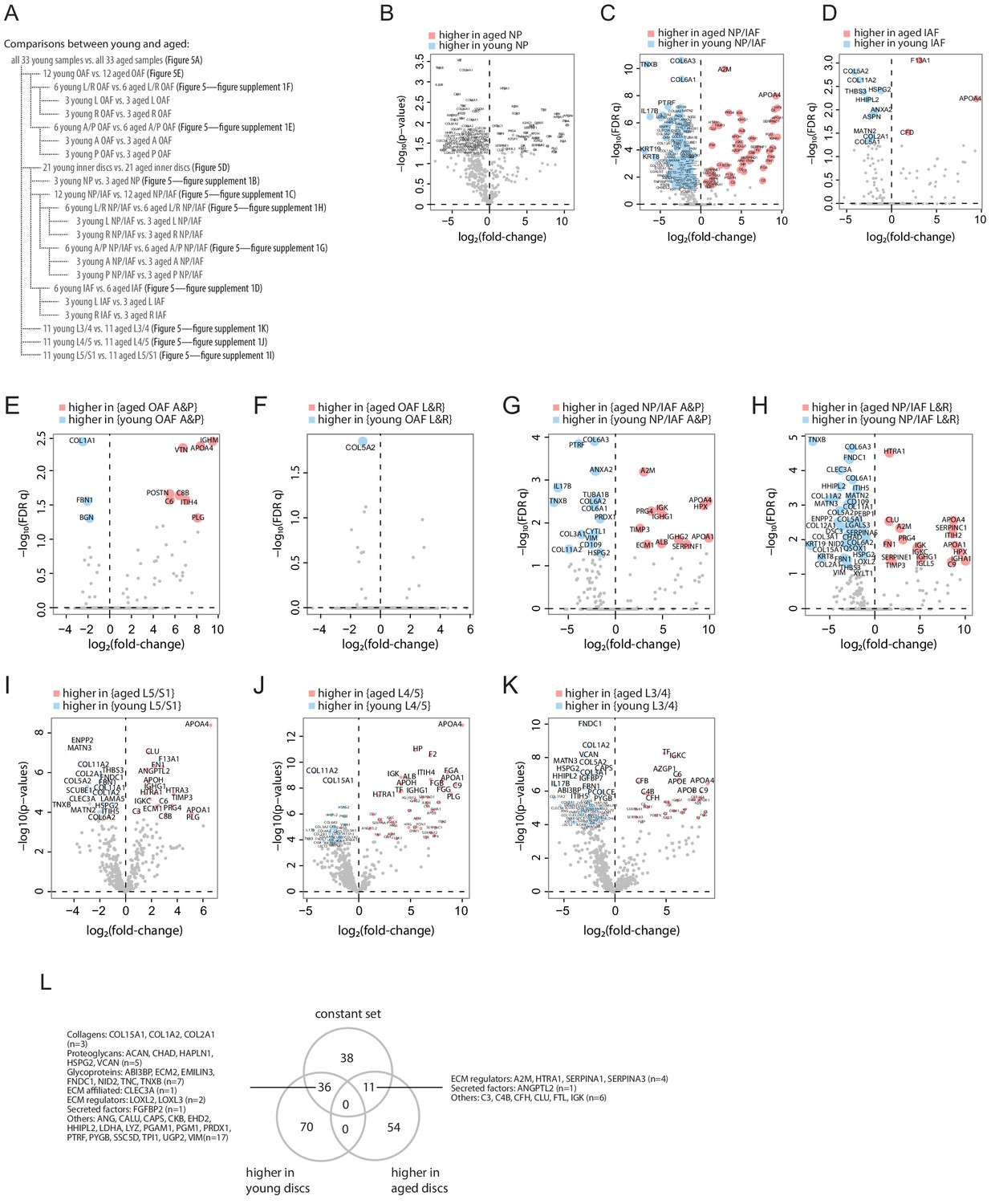
(A) Schematic diagrams showing the comparisons between young and aged profiles. (B-K) Volcano plots showing the differentially expressed proteins (DEPs) for each comparison listed in (A). (L) Venn diagram showing the overlaps of the DEPs between all young and all aged discs (from Figure 5A) and the constant set in the young discs (Figure 3D).
Figure 6 with 1 supplement
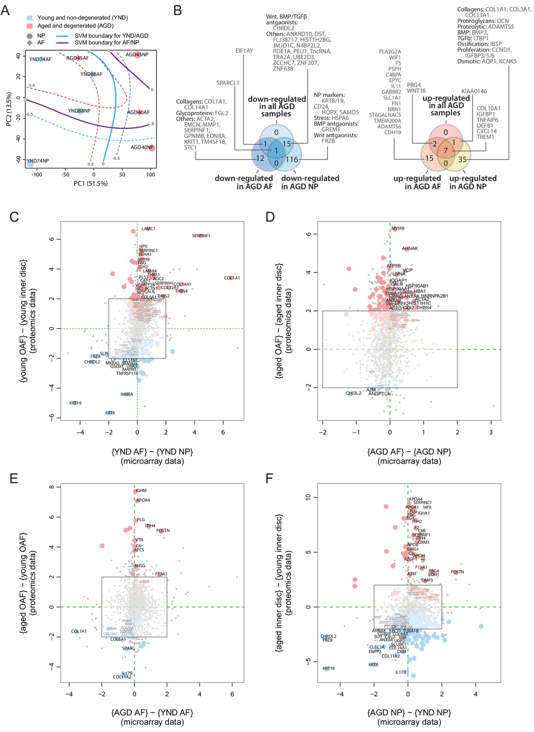
Concordance between static spatial proteomic and transcriptome data.
(A) A principal component analysis (PCA) plot of the eight transcriptomic profiles. Curves represent support vector machine (SVM) boundaries between patient-groups or compartments. (B) Venn diagrams showing the partitioning of the young/aged DEGs into contributions from inner disc regions and OAF. Left: downregulated in AGD samples; right: upregulated. (C) Transcriptome data from the NP and AF of two young individuals were compared to the proteomic data, with coloured dots representing identified proteins also expressed at the transcriptome level. (D) Transcriptome and proteome comparison of aged OAF and NP. (E) Transcriptome and proteome comparison of young and aged OAF. (F) Transcriptome and proteome comparison of young and aged NP.
Figure 6—figure supplement 1
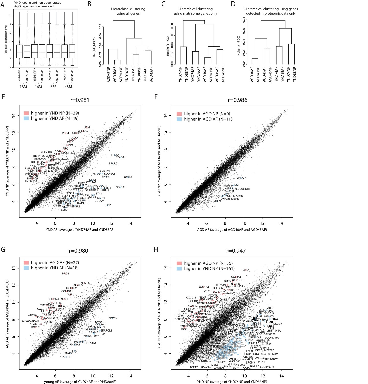
Microarray transcriptomic data of the NP and AF from four individuals, two of which are young and non-degenerated and the other two aged and degenerated.
(A) Boxplots of the normalised data show per-sample distribution of genome-wide expression profiles. (B)-(D) Hierarchical clustering of the eight microarray samples, based on genome-wide genes (B), matrisome genes (C), or the genes detected by proteomic data only (D). (E)-(H) Scatter plots of probesets between the average expressions of two groups. Red colour indicates higher expression in the y-axis samples, and blue indicates higher expression in the x-axis samples. A log2(fold-change) of >3 and average expression >10 were used as cutoffs. Multiple instances of a differentially expressed gene are due to multiple probesets design of the array.
Figure 7 with 2 supplements
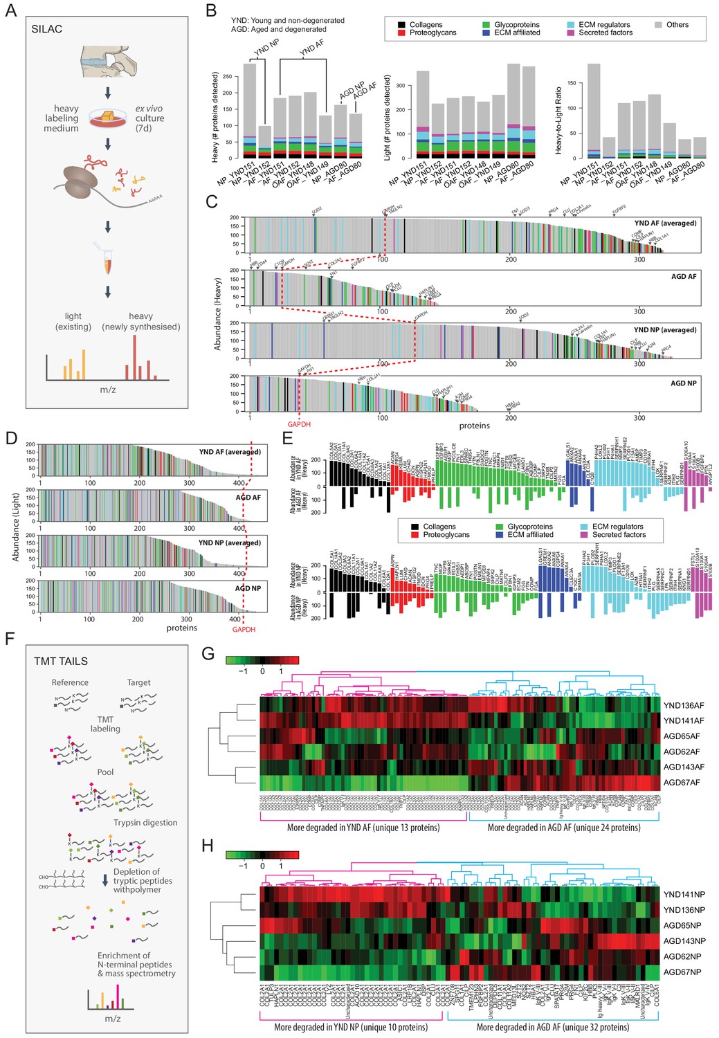
The dynamic proteome of the intervertebral disc shows less biosynthesis of proteins and more degradative events in aged tissues.
(A) Schematic showing pulse-SILAC labelling of ex-vivo cultured disc tissues where heavy Arg and Lys are incorporated into newly made proteins (heavy), and pre-existing proteins remaining unlabelled (light). NP and AF tissues from young (n = 3) and aged (n = 1) were cultured for 7 days in hypoxia prior to MS. (B) Barcharts showing the number of identified non-matrisome (grey) and matrisome (coloured) existing proteins (middle panel); newly synthesised proteins (left panel), and the heavy/light ratio (right panel) for each of the samples. (C) The quantities of each of the heavy labelled (newly synthesised) proteins identified for each of the four groups were averaged, and then plotted in descending order of abundance. It shows that YND AF and NP synthesise higher numbers of proteins than the AGD AF and NP. The red dotted reference line shows the expression of GAPDH. (D) The quantities of each of the light (existing) proteins identified for each group was averaged, and then plotted in descending order of abundance which shows that there are similar levels of existing proteins in the four pooled samples. (E) The matrisome proteins of (C) were singled out for display. The abundance of these proteins in YND samples were generally higher across all types of matrisome proteins than the AGD, with the exceptions of aged related proteins. (F) Schematic showing the workflow of degradome analysis by N-terminal amine isotopic labelling (TAILS) for the identification of cleaved neo N-terminal peptides. (G) Heatmap showing the identification of cleaved proteins ranked according to tandem mass tag (TMT) isobaric labelling of N-terminal peptides in AF. Data is expressed as the log2(ratio) of N-terminal peptides. (H) Heatmap showing the identification of cleaved proteins ranked according to tandem mass tag (TMT) isobaric labelling of N-terminal peptides in NP. Data is expressed as the log2(ratio) of N-terminal peptides. AGD143 in (G and H) is aged but not degenerated (trauma).
Figure 7—figure supplement 1
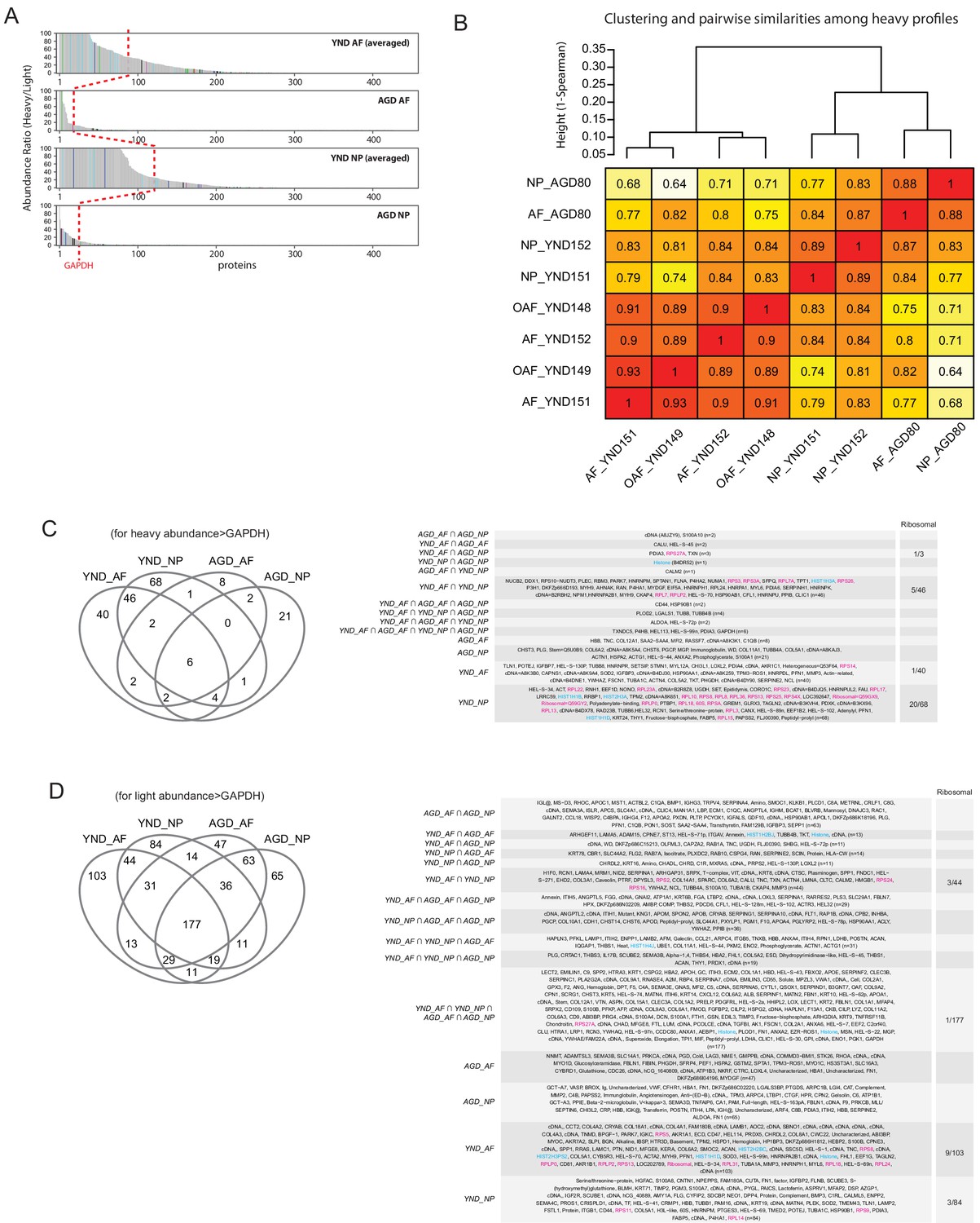
SILAC data.
(A) The heavy-to-light ratios for each of the four groups were averaged, and then plotted in descending order of abundance. The red dotted reference line shows the expression of GAPDH. (B) Clustering (based on 1-Spearman as distance metrics and complete linkage) of the eight heavy SILAC profiles shows that 'NP_YND151' and 'NP_YND152' have the tendency to cluster together, despite their difference in the numbers of detected proteins (Figure 7B left). Numbers in cells are Spearman correlation coefficients (based on non-missing values in both profiles under comparison) between pairs of profiles. (C) Venn diagram showing the overlap of proteins detected by the heavy SILAC profiles with abundance greater than GAPDH. The specific proteins in overlap are shown in the table to the right. (D) Venn diagram showing the overlap of proteins detected by the light SILAC profiles with abundance greater than GAPDH. The specific proteins in overlap are shown in the table to the right. Ribosomal proteins are highlighted in red.
Figure 7—figure supplement 2
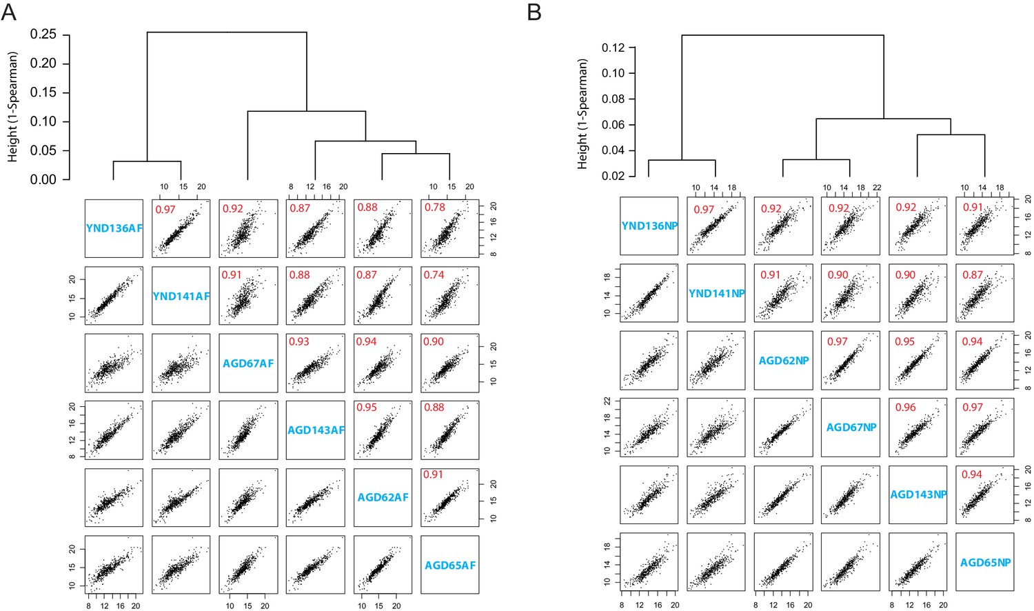
Degradome data.
(A) Hierarchical cluster (upper panel) and pairwise scatter plot (lower panel) of the degradome profiles in the AF. Numbers in red are the Spearman correlation coefficient. (B) Hierarchical cluster (upper panel) and pairwise scatter plot (lower panel) of the degradome profiles in the NP. Numbers in red are the Spearman correlation coefficient.
Figure 8 with 1 supplement
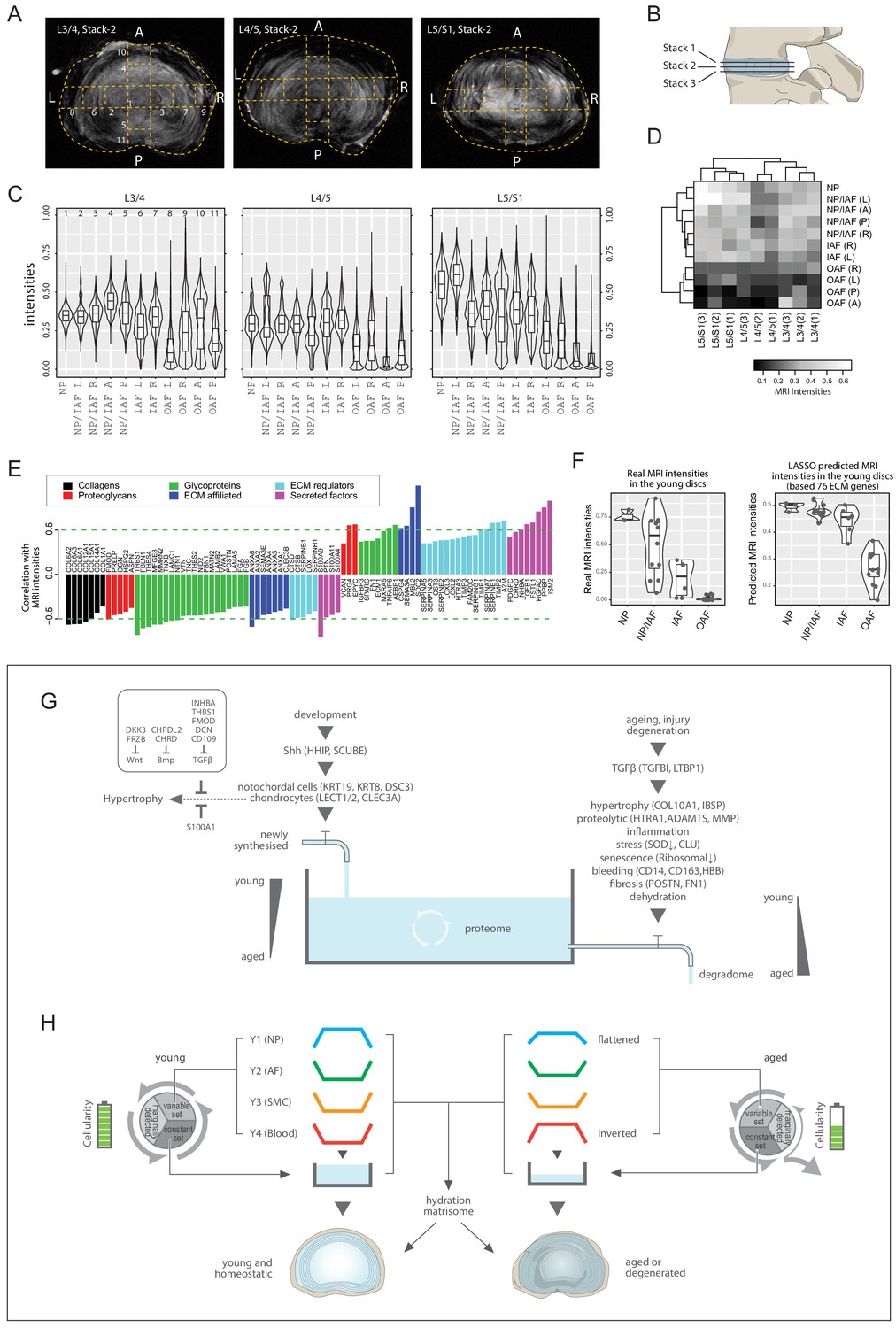
MRI intensities and their correlation with the proteomic data.
(A) The middle MRI stack of each disc level in the aged cadaveric sample. (B) Schematic of the disc showing the three stacks of MRI images per disc. (C) Violin plots showing the pixel intensities within each location per disc level, corresponding to the respective locations taken for mass spectrometry measurements. Each violin-plot is the aggregate of three stacks of MRIs per disc. (D) A heatmap bi-clustering of levels and compartments based on the MRI intensities. (E) The hydration extracellular matrices (ECMs): the ECM proteins most positively and negatively correlated with MRI. (F) The 3T MRI intensities of the young discs across the compartments (left), and the predicted MRI intensities based on a LASSO regression model trained on the hydration ECMs (right). (G) A water-tank model of the dynamics in disc proteomics showing the balance of the proteome is maintained by adequate anabolism to balance catabolism. (H) Diagram showing the partitioning of the detected proteins into variable and constant sets, whereby four modules characterising the young healthy disc were further derived; and showing their changes with ageing. SMC: smooth muscle cell markers.
Figure 8—figure supplement 1
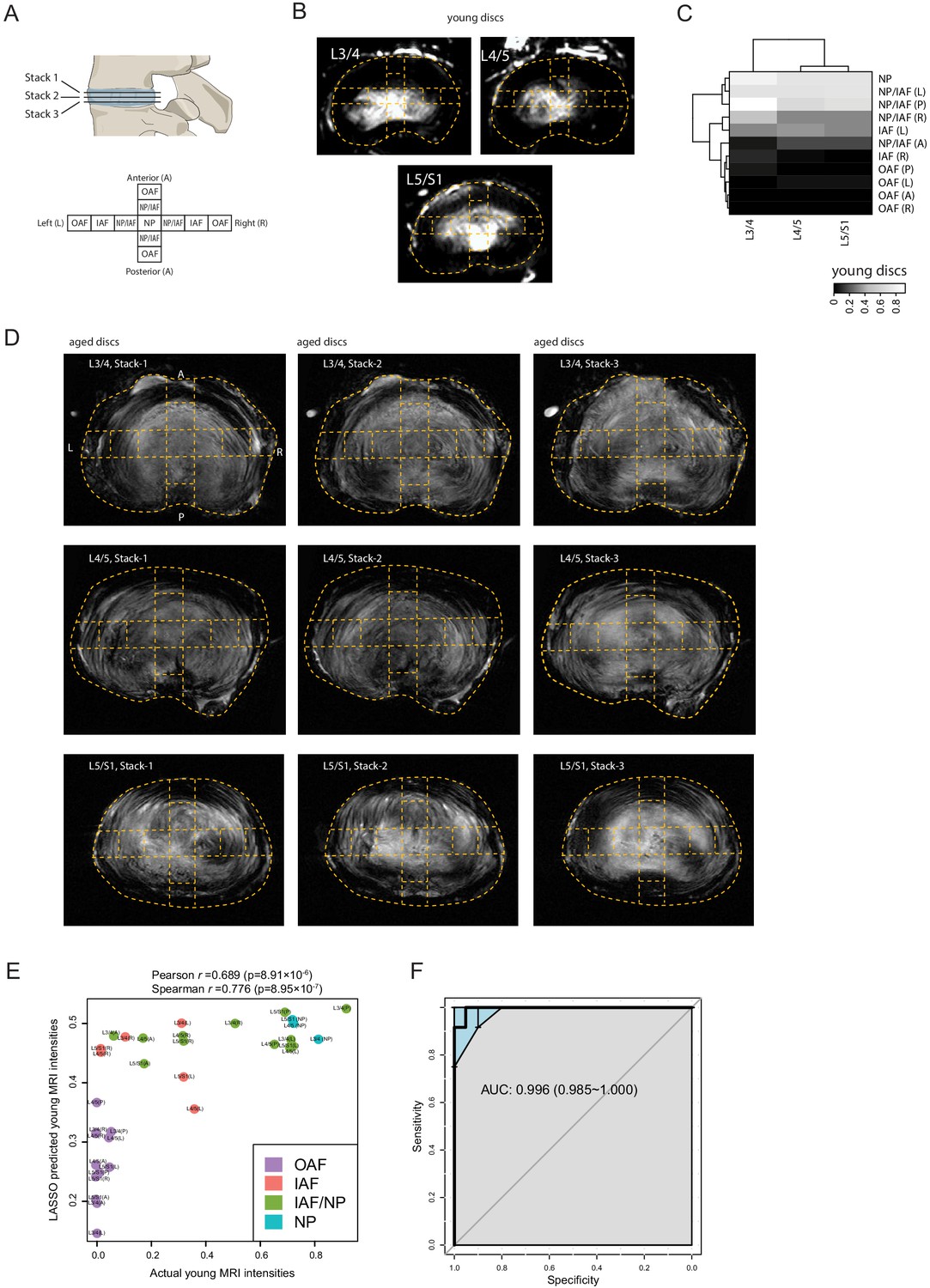
MRI-molecule connections.
(A) Diagram showing the stacks of MRI per disc level and the 11 locations per disc. (B) Dashed curves overlaying the young discs’ 3T MRI images, showing the compartments taken for proteomic profiling. (C) A heatmap with compartment and level bi-clustering, showing the relationship between regional MRI intensities. (D) Stacks of MRI images of the aged sample. (E) Scatter-plot showing the actual original MRI intensities of the young discs, and their predicted intensities of an LASSO model trained based on the ECM proteins most correlated with the aged disc MRI intensities. (F) A receiver operating characteristic (ROC) curve of the predicted MRI intensities between inner disc regions and OAF. AUC, area under the curve.
Tables
Table 1
Summary of disc samples in DIPPER.
| Samples | Age | Sex | Disc level/s | Disc regions | Reason for surgery |
|---|---|---|---|---|---|
| Cadaver samples | |||||
| Young spine | 16 | M | L3/4, L4/5, L5/S1 | NP, NP/IAF, IAF, OAF | N/A |
| Aged spine | 59 | M | L3/4, L4/5, L5/S1 | NP, NP/IAF, IAF, OAF | N/A |
| Transcriptome samples | |||||
| YND74 | 17 | M | L1/2 | NP, OAF | Scoliosis |
| YND88 | 16 | M | L1/2 | NP, OAF | Scoliosis |
| AGD40 | 62 | F | L4/5 | NP, OAF | Degeneration |
| AGD45 | 47 | M | L4/5 | NP, OAF | Degeneration |
| SILAC samples | |||||
| YND148 | 19 | F | L2/3 | OAF | Scoliosis |
| YND149 | 15 | F | L1/2 | OAF | Scoliosis |
| YND151 | 15 | F | L1/2 | NP, OAF | Scoliosis |
| YND152 | 14 | F | L1/2 | NP, OAF | Scoliosis |
| AGD80 | 63 | M | L4/5 | NP, OAF | Degeneration |
| Degradome samples | |||||
| YND136 | 17 | F | L1/2 | NP, OAF | Scoliosis |
| YND141 | 20 | F | L1/2 | NP, OAF | Scoliosis |
| AGD143 | 53 | M | L1/2 | NP, OAF | Trauma |
| AGD62 | 55 | F | L5/S1 | NP, OAF | Degeneration |
| AGD65 | 68 | F | L4/5 | NP, OAF | Degeneration |
| AGD67 | 55 | M | L4/5 | NP, OAF | Degeneration |
Table 2
Commonly expressed extracellular matrix (ECM) and associated proteins across all 66 profiles in the spatial proteome.
| Categories (Number of proteins) | Protein names |
|---|---|
| Core matrisome | |
| Collagens (13) | COL1A1/2, COL2A1, COL3A1, COL5A1, COL6A1/2/3, COL11A1/2, COL12A1, COL14A1, COL15A1 |
| Proteoglycans (14) | ACAN, ASPN, BGN, CHAD, DCN, FMOD, HAPLN1, HSPG2, LUM, OGN, OMD, PRELP, PRG4, VCAN |
| Glycoproteins (34) | ABI3BP, AEBP1, CILP, CILP2, COMP, DPT, ECM2, EDIL3, EFEMP2, EMILIN1, FBN1, FGA, FGB, FN1, FNDC1, LTBP2, MATN2/3, MFGE8, MXRA5, NID2, PCOLCE, PCOLCE2, PXDN, SMOC1/2, SPARC, SRPX2, TGFBI, THBS1/2/4, TNC, TNXB |
| Other matrisome | |
| ECM affiliated proteins (10) | ANXA1/2/4/5/6, CLEC11A, CLEC3A/B, CSPG4, SEMA3C |
| ECM regulators (16) | A2M, CD109, CST3, F13A1, HTRA1, HTRA3, ITIH5, LOXL2/3, PLOD1, SERPINA1/3/5, SERPINE2, SERPING1, TIMP1 |
| Secreted factors (2) | ANGPTL2, FGFBP2 |
Additional files
-
Supplementary file 1
Processed data of the 66 LC-MS/MS static spatial proteome profiles.
- https://cdn.elifesciences.org/articles/64940/elife-64940-supp1-v3.xlsx
-
Supplementary file 2
Differentially expressed proteins (DEPs) among pairs of sample groups within the 33 young static spatial disc profiles.
- https://cdn.elifesciences.org/articles/64940/elife-64940-supp2-v3.xlsx
-
Supplementary file 3
Differentially expressed proteins (DEPs) among pairs of sample groups within the 33 aged static spatial disc profiles.
- https://cdn.elifesciences.org/articles/64940/elife-64940-supp3-v3.xlsx
-
Supplementary file 4
Differentially expressed proteins (DEPs) between young and aged sample groups of static spatial proteomes.
- https://cdn.elifesciences.org/articles/64940/elife-64940-supp4-v3.xlsx
-
Supplementary file 5
Significantly enriched gene ontology (GO) terms associated with proteins expressed higher in all young or all aged discs.
- https://cdn.elifesciences.org/articles/64940/elife-64940-supp5-v3.xlsx
-
Transparent reporting form
- https://cdn.elifesciences.org/articles/64940/elife-64940-transrepform-v3.pdf
Download links
A two-part list of links to download the article, or parts of the article, in various formats.
Downloads (link to download the article as PDF)
Open citations (links to open the citations from this article in various online reference manager services)
Cite this article (links to download the citations from this article in formats compatible with various reference manager tools)
DIPPER, a spatiotemporal proteomics atlas of human intervertebral discs for exploring ageing and degeneration dynamics
eLife 9:e64940.
https://doi.org/10.7554/eLife.64940


