Strategically managing learning during perceptual decision making
- Department of Molecular and Cellular Biology, Harvard University, United States
- Center for Brain Science, Harvard University, United States
- Department of Experimental Psychology, University of Oxford, United Kingdom
Figures
Figure 1 with 7 supplements
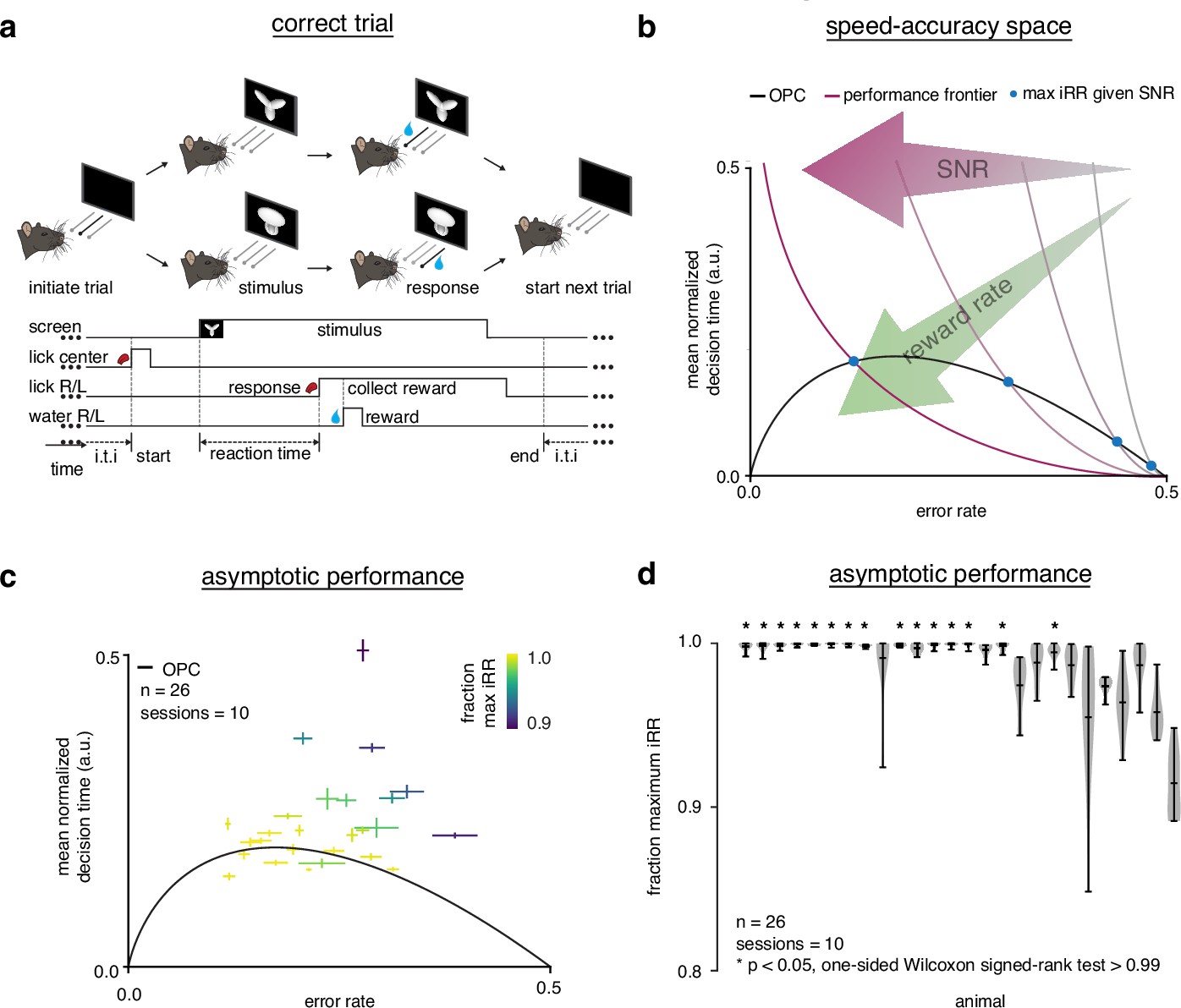
Trained rats solve the speed-accuracy trade-off.
(a) Rat initiates trial by licking center port, one of two visual stimuli appears on the screen, rat chooses correct left/right response port for that stimulus and receives a water reward. (b) Speed-accuracy space: a decision making agent’s and mean normalized (a normalization of based on the average timing between one trial and the next, see Methods). Assuming a simple drift-diffusion process, agents that maximize (see Methods) must lie on an optimal performance curve (OPC, black trace) (Bogacz et al., 2006). Points on the OPC relate error rate to mean normalized decision time, where the normalization takes account of task timing parameters (e.g. average response-to-stimulus interval). For a given SNR, an agent’s performance must lie on a performance frontier swept out by the set of possible threshold-to-drift ratios and their corresponding error rates and mean normalized decision times. The intersection point between the performance frontier and the OPC is the error rate and mean normalized decision time combination that maximizes for that SNR. Any other point along the performance frontier, whether above or below the OPC, will achieve a suboptimal. Overall, increases toward the bottom left with maximal instantaneous reward rate at error rate = 0.0 and mean normalized decision time = 0.0. (c) Mean performance across 10 sessions for trained rats () at asymptotic performance plotted in speed-accuracy space. Each cross is a different rat. Color indicates fraction of maximum instantaneous reward rate () as determined by each rat’s performance frontier. Errors are bootstrapped SEMs. (d) Violin plots depicting fraction of maximum, a quantification of distance to the OPC, for same rats and same sessions as c. Fraction of maximum is a comparison of an agent’s current with its optimal given its inferred SNR. Approximately 15 of 26 (∼60%) of rats attain greater than 99% fraction maximum for their individual inferred SNRs. * denotes p < 0.05 one-tailed Wilcoxon signed-rank test for mean >0.99.
Figure 1—figure supplement 1

Task schematic for error trials.
Error trial: rat chooses incorrect left/right response port and incurs a timeout period.
Figure 1—figure supplement 2

Fraction of ignored trials during learning.
(a) Schematic of an ignore trial: rat does not choose a left/right response port and receives no feedback. (b) Fraction of trials ignored (ignored trials/(correct + incorrect + ignored trials)) during learning for animals encountering the task for the first time (stimulus pair 1). (c) Fraction of trials ignored for animals learning stimulus pair 2 after training on stimulus pair 1.
Figure 1—figure supplement 3
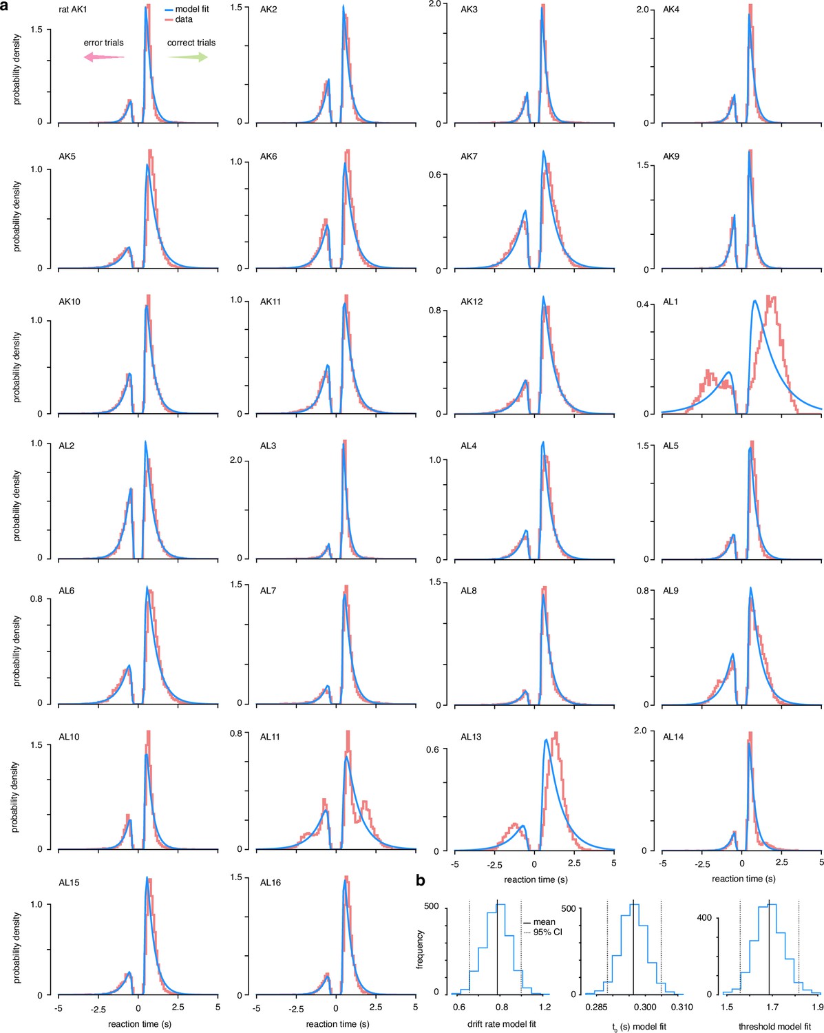
Drift-diffusion model data fits.
(a) The accuracy and reaction time data from 26 trained rats was fit to a simple drift-diffusion model using the hierarchical Bayesian estimation of the drift-diffusion model (HDDM) package (Wiecki et al., 2013). (b) Estimated posterior distributions of parameter values across all animals.
Figure 1—figure supplement 4
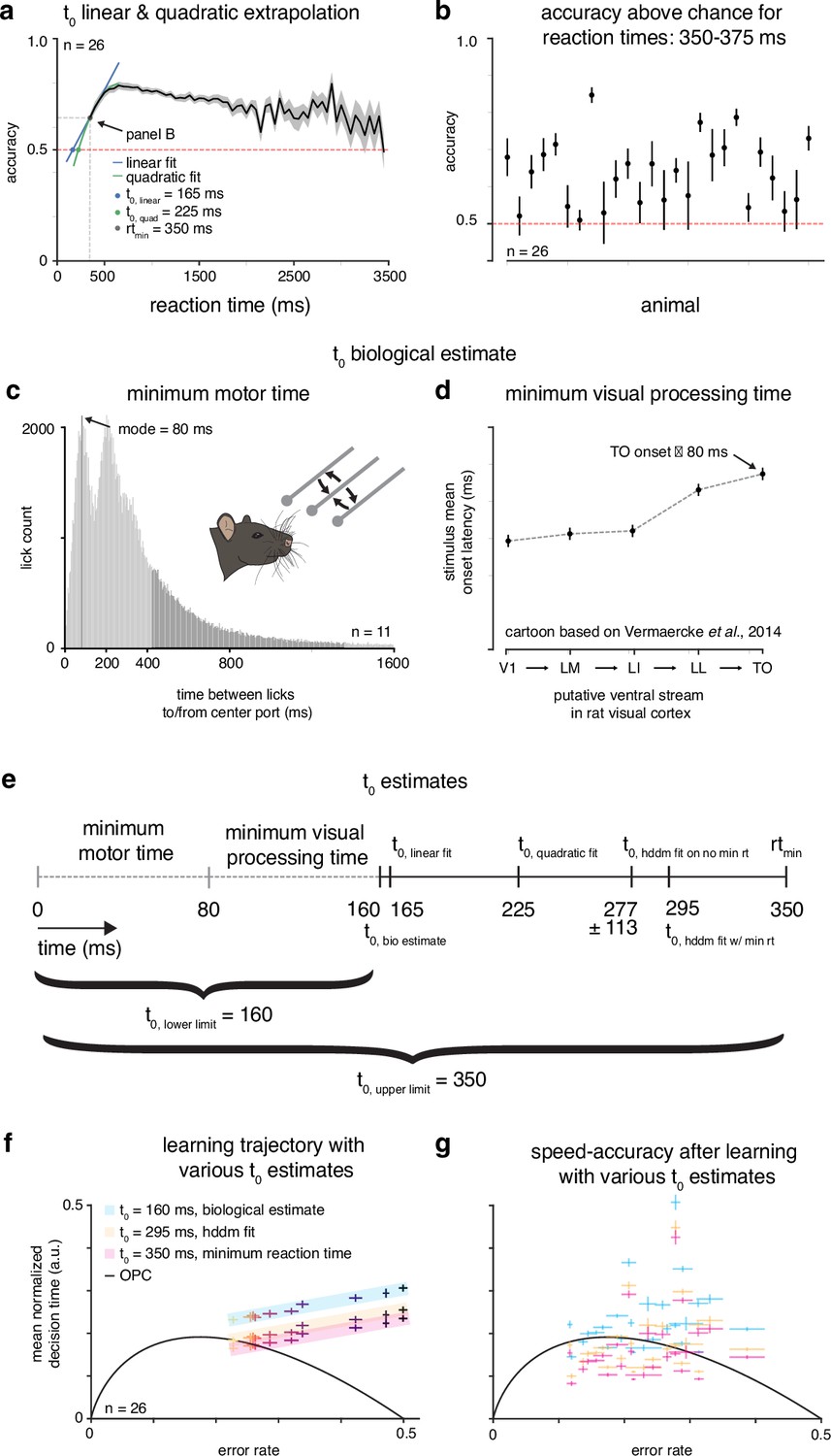
Estimating .
(a) Linear and quadratic extrapolations to accuracy as a function of reaction time. The T0 estimate is when each extrapolation intersects chance accuracy (0.5). (b) Mean accuracy for trials with reaction times 350–375 ms for rats. (c) Minimum motor time estimated by looking at first peak of time between licks to/from center port for rats. (d) Cartoon of stimulus onset latency across visual areas from Vermaercke et al., 2014 to estimate minimum visual processing time. (e) Diagram of T0 estimates, with an upper limit (minimum reaction time) and lower limit (minimum motor time + minimum visual processing time). (f) Mean learning trajectory for rats with various t0 estimates. (g) Subjects () in speed-accuracy space with various T0 estimates.
Figure 1—figure supplement 5

Analysis of voluntary intertrial intervals (ITIs).
(a) Histogram of voluntary ITIs (time in addition to mandatory experimentally determined and ) for rats across 10 sessions for previous correct (blue) and previous error (red) ITIs. Voluntary ITIs are spaced every 500 ms because of violations to the ‘cannot lick’ period. Inset: proportion of voluntary ITIs below 500, 1000, and 2000 ms boundaries. (b) Median voluntary ITIs up too 500, 1000, and 2000 ms boundaries. (c) Overlay of voluntary ITIs spaced 500 ms apart after previous correct trials. (d) Overlay of voluntary ITIs spaced 500 ms apart after previous error trials.
Figure 1—figure supplement 6
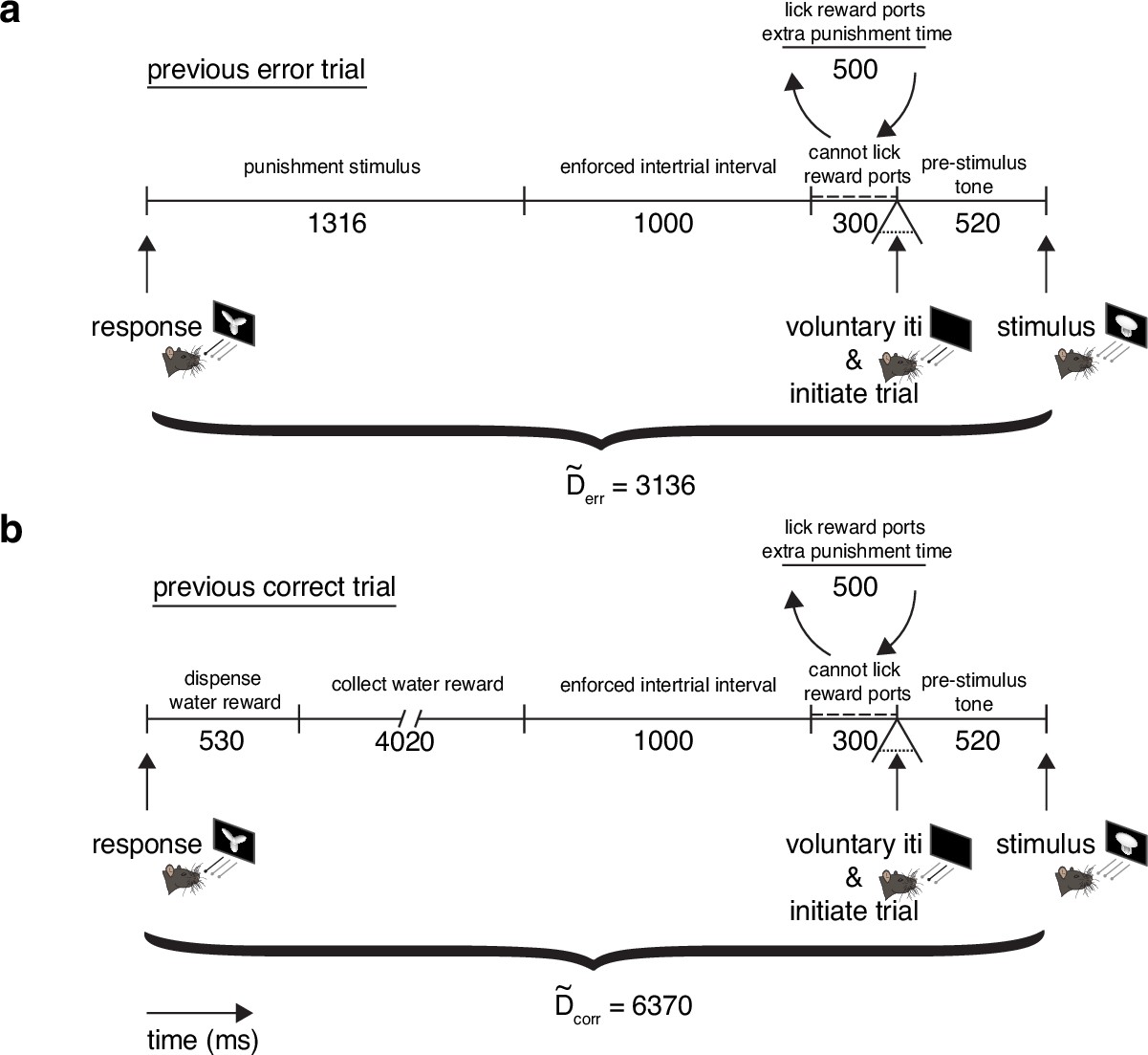
Mandatory post-error () and post-correct () response-to-stimulus interval times.
(a) Diagram of intertrial interval (ITI) after previous error trial. All times (punishment stimulus, enforced intertrial interval, cannot lick reward ports, and pre-stimulus time) were verified based on timestamps on experimental file logs. After the punishment stimulus and enforced intertrial interval, there is a 300 ms period where rats cannot lick the reward ports. If violated, 500 ms are added to the intertrial interval followed by another 300 ms ‘cannot lick’ period. In addition to this restriction, rats may take as much voluntary time between trials as they wish. Any violation of the ‘cannot lick’ period is counted as voluntary time, and only the minimum mandatory time of 3136 ms is counted for . (b) Diagram of ITI after previous correct trial. All times (dispense water reward, collect water reward, enforced intertrial interval, cannot lick reward ports, pre-stimulus time) were verified based on timestamps on experimental file logs. The same ‘cannot lick’ period is present as in a. All times (dispense water reward, collect water reward, enforced intertrial interval, cannot lick reward ports, pre-stimulus time) were verified based on timestamps on experimental file logs. Any violation of the ‘cannot lick’ period is counted as voluntary time, and only the minimum mandatory time of 6370 ms is counted for .
Figure 1—figure supplement 7

Reward rate sensitivity to and voluntary intertrial interval (ITI).
(a) Fraction of maximum instantaneous reward rate across rats over 10 sessions at asymptotic performance over possible voluntary ITI values of 0–1000 ms and over the minimum and maximum estimated T0 values. (b) Fraction of maximum instantaneous reward rate across rats over 10 sessions at asymptotic performance over possible T0 values from 160 to 350 ms (min to max estimated T0 values) and over the median voluntary ITIs with 500, 1000, and 2000 ms boundaries. (c) Fraction of maximum instantaneous reward rate across rats as a function of normalized training time during learning period and possible voluntary ITIs from 0 to 2000 ms calculated with the T0 minimum of 160 ms. The gray curves represent a weighted average over previous correct/error median voluntary ITIs over normalized training time. Contours with different fractions of maximum instantaneous reward rate in pink. (d) Same as in c but calculated with T0 maximum of 350 ms.
Figure 2 with 1 supplement
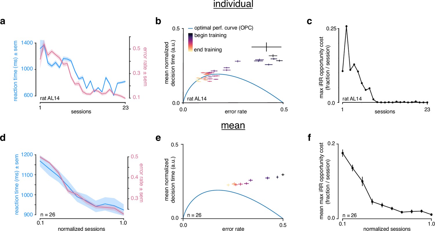
Rats do not greedily maximize instantaneous reward rate during learning.
(a) Reaction time (blue) and error rate (pink) for an example subject (rat AL14) across 23 sessions. (b) Learning trajectory of individual subject (rat AL14) in speed-accuracy space. Color map indicates training time. Optimal performance curve (OPC) in blue. (c) Maximum opportunity cost (see Methods) for individual subject (rat AL14). (d) Mean reaction time (blue) and error rate (pink) for rats during learning. Sessions across subjects were transformed into normalized sessions, averaged and binned to show learning across 10 bins. Normalized training time allows averaging across subjects with different learning rates (see Methods). (e) Learning trajectory of rats in speed-accuracy space. Color map and OPC as in a. (f) Maximum opportunity cost of rats in b throughout learning. Errors reflect within-subject session SEMs for a and b and across-subject session SEMs for d, e, and f.
Figure 2—figure supplement 1

Comparison of training regimes.
(a) ‘Canonical only’: rats trained to asymptotic performance with only front-view image of each of the two stimuli. ‘Size and rotation’: rats first shown front-view image of stimuli. After reaching criterion (), size staircased. Following criterion, rotation staircased. Upon criterion, stimuli randomly drawn across size and rotation. (b) Learning trajectory in speed-accuracy space over normalized training time for rats trained with the ‘size and rotation’ (left panel) and the ‘canonical only’ training regimes (right panel). (c) Average location in speed-accuracy space for 10 sessions after asymptotic performance for individual rats in both training regimes, as in b. (d) Mean accuracy over learning (left panel) and for 5 sessions after asymptotic performance (right panel) for rats trained with the ‘size and rotation’ () and the ‘canonical only’ (n=8) training regimes. (e) Mean reaction time. (f) Mean fraction max . (g) Mean total trials per session. (h) Mean voluntary intertrial interval up to 500 ms after error trials. (i) Mean fraction ignored trials. All errors are SEM. Significance in right panels of d–i determined by Wilcoxon rank-sum test with p<0.05.
Figure 3 with 1 supplement
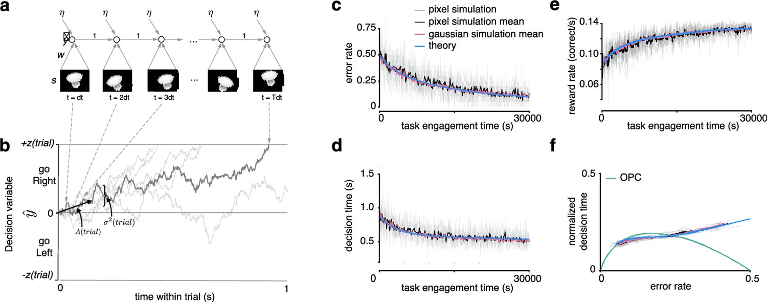
Recurrent neural network and learning drift diffusion model (DDM).
(a) Roll out in time of recurrent neural network (RNN) for one trial. (b) The decision variable for the recurrent neural network (dark gray), and other trajectories of the equivalent DDM for different diffusion noise samples (light gray). (c, d, e) Changes in , , and over a long period of task engagement in the RNN (light gray, pixel simulation individual traces; black, pixel simulation mean; pink, Gaussian simulation mean) compared to the theoretical predictions from the learning DDM (blue). (f) Visualization of traces in c and d in speed-accuracy space along with the optimal performance curve (OPC) in green. The threshold policy was set to be -sensitive for c–f.
Figure 3—figure supplement 1
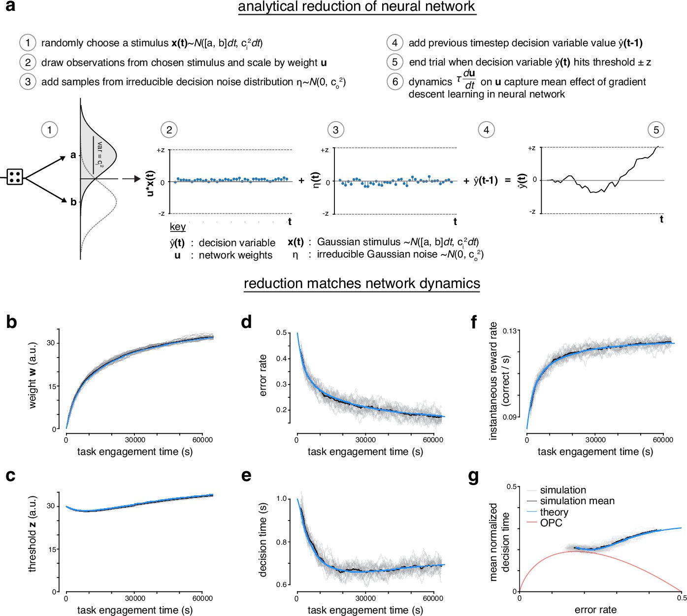
Analytical reduction of linear drift-diffusion model (LDDM) matches error-corrective learning neural network dynamics during learning.
(a) The recurrent linear neural network can be analytically reduced. In the reduction, the decision variable draws an observation from one of two randomly chosen Gaussian ‘stimuli’. The observations are scaled by a perceptual weight. After the addition of some irreducible noise, the value of the decision variable at previous time step is added to the current time step. A trial ends once the decision variable hits a predetermined threshold. The dynamics of the perceptual weight capture the mean effect of gradient descent learning in the recurrent linear neural network. (b) Weight w of neural network across task engagement time for multiple simulations of the network (gray), the mean of the simulations (black), and the analytical reduction of the network (blue). (c) Same as in b but for the threshold z. (d) Same as in b but for the error rate. (e) Same as in b but for the decision time. (f) Same as in b but for the instantaneous reward rate (correct trials per second). (g) Learning trajectory in speed-accuracy space for simulations, simulation mean, and analytical reduction (theory). Optimal performance curve (OPC) is shown in red.
Figure 4 with 5 supplements
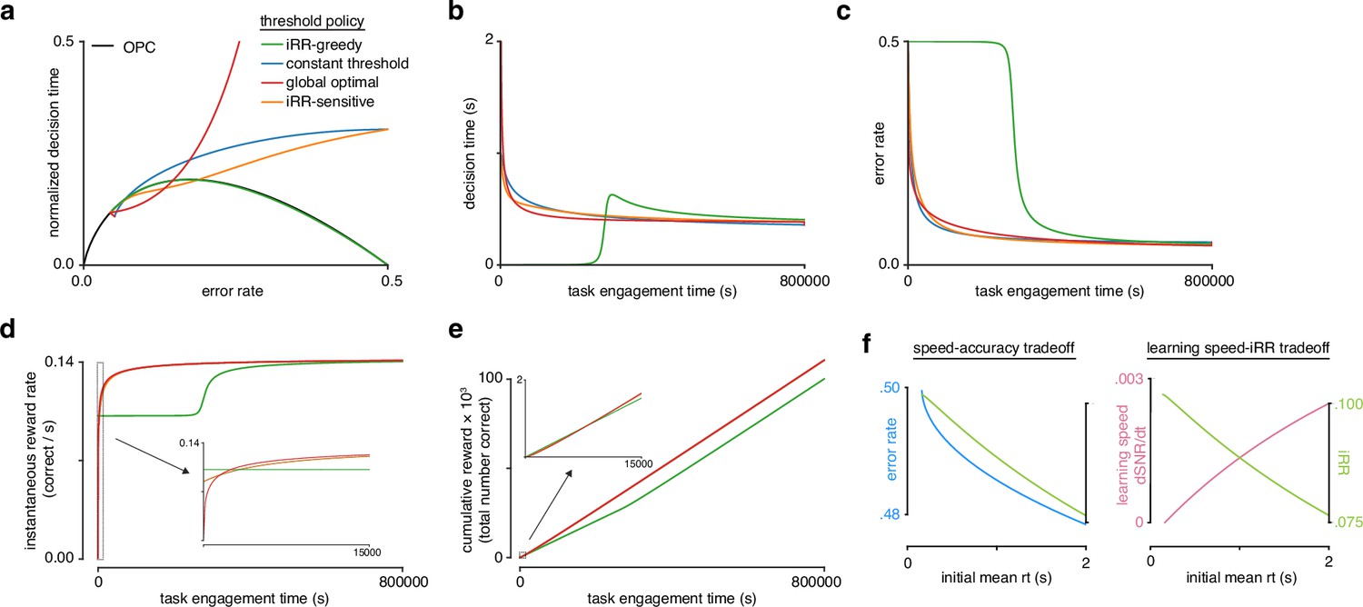
Model reveals rat learning dynamics lead to higher instantaneous reward rate and long-term rewards than greedily maximizing instantaneous reward rate.
(a) Model learning trajectories in speed-accuracy space plotted against the optimal performance curve (OPC) (black). (b) Decision time through learning for the four different threshold policies in a. (c) Error rate throughout learning for the four different threshold policies in a. (d) Instantaneous reward rate as a function of task engagement time for the full learning trajectory and a zoom-in on the beginning of learning (inset). (e) Cumulative reward as a function of task engagement time for the full learning trajectory and a zoom-in on the beginning of learning (inset). Threshold policies: -greedy (green), constant threshold (blue), -sensitive (orange), and global optimal (red). (f) In the speed-accuracy trade-off (left), (blue) decreases with increasing initial mean (green) at high error rates (∼0.5) also decreases with increasing initial mean . Thus, at high , an agent solves the speed-accuracy trade-off by choosing fast that result in higher and maximize . In the learning speed/ trade-off (right), initial learning speed (, pink) increases with increasing initial mean , whereas (green) follows the opposite trend. Thus, an agent must trade in order to access higher learning speeds. Plots generated using linear drift-diffusion model (LDDM).
Figure 4—figure supplement 1

Allowing both drift rate and threshold to vary with learning provides the best drift-diffusion model (DDM) fits.
(a) Deviance information criterion (DIC) for different hierarchical DDM (HDDM) fits to learning during stimulus pair 1 (lower value indicates a better fit). The models were fit to the first 1000 and last 1000 trials for every animal using the HDDM framework (Wiecki et al., 2013). Different parameters were allowed to vary with learning phase while the rest were fixed across learning phase. We fit three simple DDMs, one model that only allowed drift rate variability to vary with learning, three DDMs that included a fixed drift rate variability across learning phase (‘include drift variability’), and three DDMs where drift rate variability varied with learning in addition to different combinations of drift rate and threshold. The best models were those that allowed both drift rate and threshold to vary with learning. Including drift rate variability and allowing it to also vary with learning phase did not improve the model fits. Parameters for these model fits are included in the subsequent figures. (b) Same as a but for stimulus pair 2. The models were fit to the last 500 trials of baseline sessions with stimulus pair 1, and the first 500 trials and last 500 trials of stimulus pair 2, with each 500 trial batch serving as a learning phase. As with stimulus pair 1, the best models were those that allowed both drift rate and threshold to vary with learning, and drift rate variability did not appear to allow a better model fit.
Figure 4—figure supplement 2
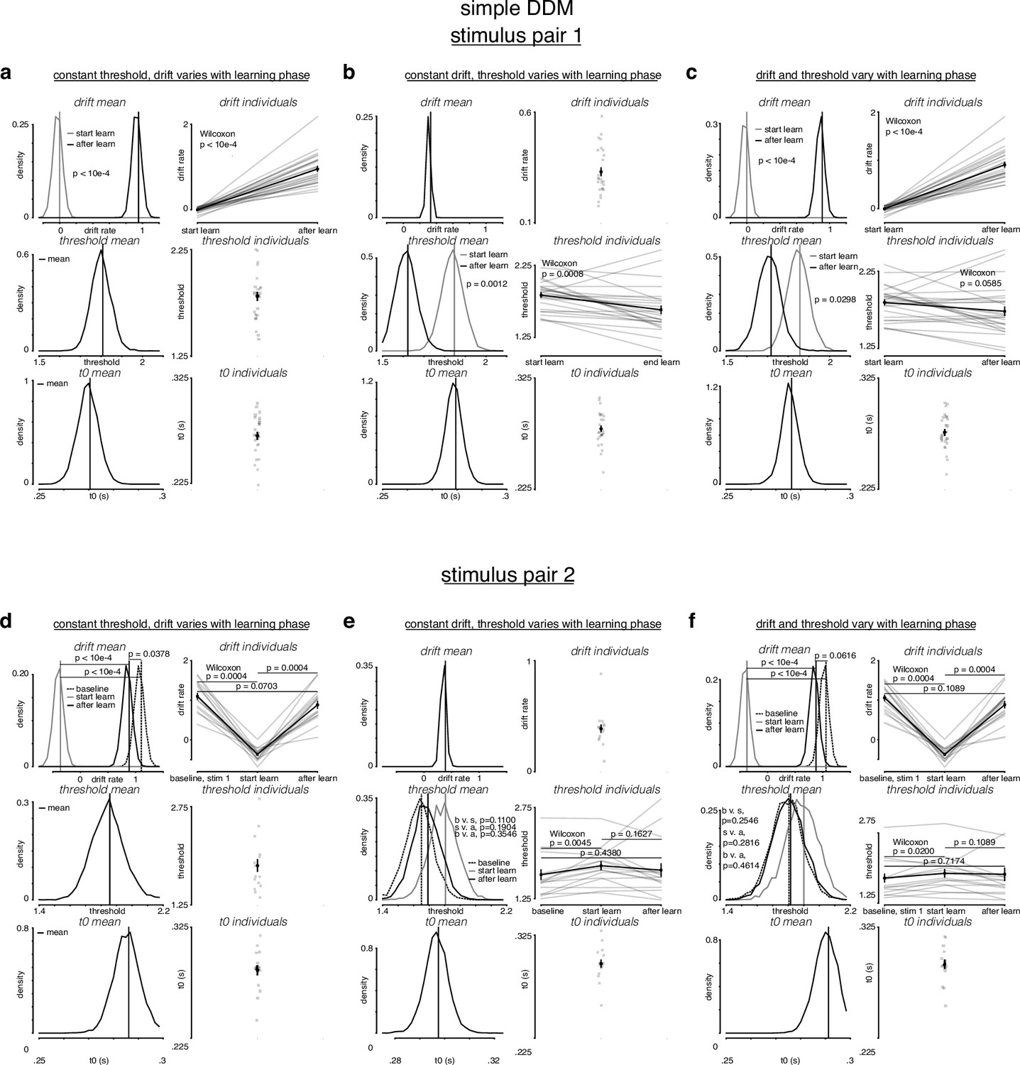
Simple drift-diffusion model (DDM) fits indicate threshold decreases and drift rate increases during learning.
(a) The learning data from stimulus pair 1 (a, b, c) and 2 (d, e, f) were fit with a simple DDM using the hierarchical DDM (HDDM) framework (Wiecki et al., 2013) as described in Figure 4—figure supplement 1. The HDDM reports posterior probability estimates for its parameters. The posterior for mean parameters across subjects is on the left of every panel, and the mean of the posterior for every individual fit is on the right of every panel. (a) While holding threshold constant, drift increased with learning. (b) While holding drift rate constant, threshold decreased with learning. (c) When allowing both drift rate and threshold to vary with learning, drift rate increased and threshold decreased with learning. (d) For stimulus pair 2, while holding threshold constant, drift increased with learning, matching its value during baseline sessions. (e) While holding drift rate constant, threshold decreased with learning, matching its value during baseline sessions. (f) When allowing both drift rate and threshold to vary with learning, drift rate increased and threshold decreased with learning, matching their values during baseline sessions. p-Values for mean estimates were calculated by taking the difference of the posteriors and counting the proportion of differences that was, depending on directionality 0. p-Values for individual estimates were calculated by taking a Wilcoxon rank-sum test across pairs.
Figure 4—figure supplement 3
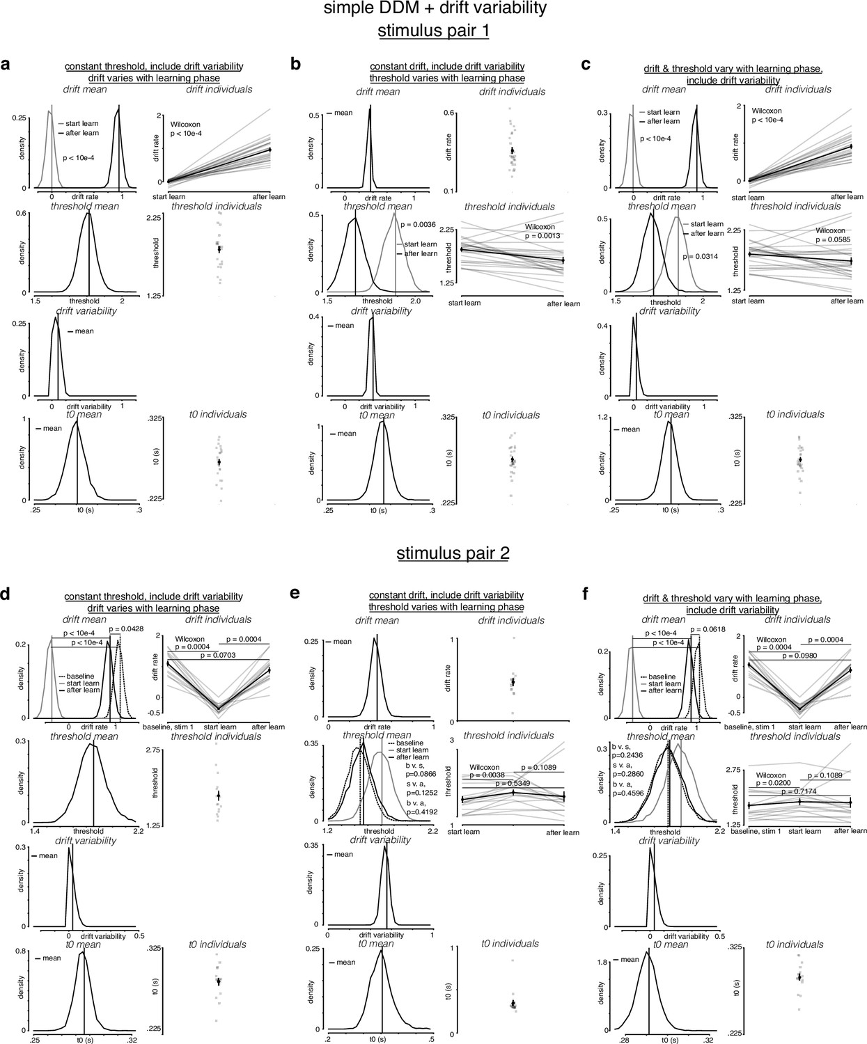
Simple drift-diffusion model (DDM) + fixed drift rate variability fits indicate threshold decreases and drift rate increases during learning.
(a) The learning data from stimulus pair 1 (a, b, c) and 2 (d, e, f) were fit with a simple DDM + fixed drift rate variability using the hierarchical DDM (HDDM) framework (Wiecki et al., 2013) as described in Figure 4—figure supplement 1. (a) While holding threshold constant, drift increased with learning. (b) While holding drift rate constant, threshold decreased with learning. (c) When allowing both drift rate and threshold to vary with learning, drift rate increased and threshold decreased with learning. Drift rate variability estimates were close to 0. (d) For stimulus pair 2, while holding threshold constant, drift increased with learning, matching its value during baseline sessions. (e) While holding drift rate constant, threshold decreased with learning, matching its value during baseline sessions. (f) When allowing both drift rate and threshold to vary with learning, drift rate increased and threshold decreased with learning, matching their values during baseline sessions. p-Values were calculated as in Figure 4—figure supplement 2.
Figure 4—figure supplement 4

Simple drift-diffusion model (DDM) + variable drift rate variability fits indicate threshold decreases and drift rate increases during learning.
(a) The learning data from stimulus pair 1 (a, b, c) and 2 (d, e, f) were fit with a simple DDM + variable drift rate variability using the hierarchical DDM (HDDM) framework (Wiecki et al., 2013) as described in Figure 4—figure supplement 1. (a) While holding threshold constant, drift and drift rate variability increased with learning. (b) While holding drift rate constant, threshold and drift rate variability decreased with learning. (c) When allowing both drift rate and threshold to vary with learning, drift rate and drift rate variability increased and threshold decreased with learning. (d) For stimulus pair 2, while holding threshold constant, drift increased with learning, matching its value during baseline sessions, while drift rate variability trended toward decreasing with stimulus pair 2. (e) While holding drift rate constant, threshold decreased with learning, matching its value during baseline sessions, and drift rate variability decreased. (f) When allowing both drift rate and threshold to vary with learning, drift rate increased and threshold decreased with learning, matching their values during baseline sessions. Drift rate variability trended toward decreasing with stimulus pair 2. p-Values were calculated as in Figure 4—figure supplement 2.
Figure 4—figure supplement 5
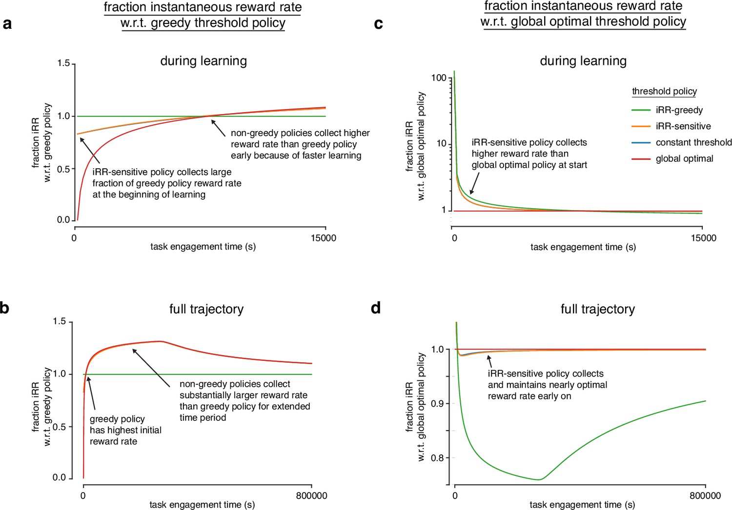
Model reveals rat learning dynamics resemble optimal trajectory without relinquishing initial rewards.
(a) Fraction of instantaneous reward rate with respect to the -greedy policy for all model threshold policies during learning. The instantaneous reward rates of all policies were normalized by the -greedy policy’s instantaneous reward rate through task engagement time. (b) Same as a but for the full trajectory of the simulation. (c) Fraction of instantaneous reward rate with respect to the global optimal policy for all model threshold policies during learning. The instantaneous reward rates of all policies were normalized by the greedy policy’s instantaneous reward rate through task engagement time. (d) Same as c but for the full trajectory of the simulation.
Figure 5
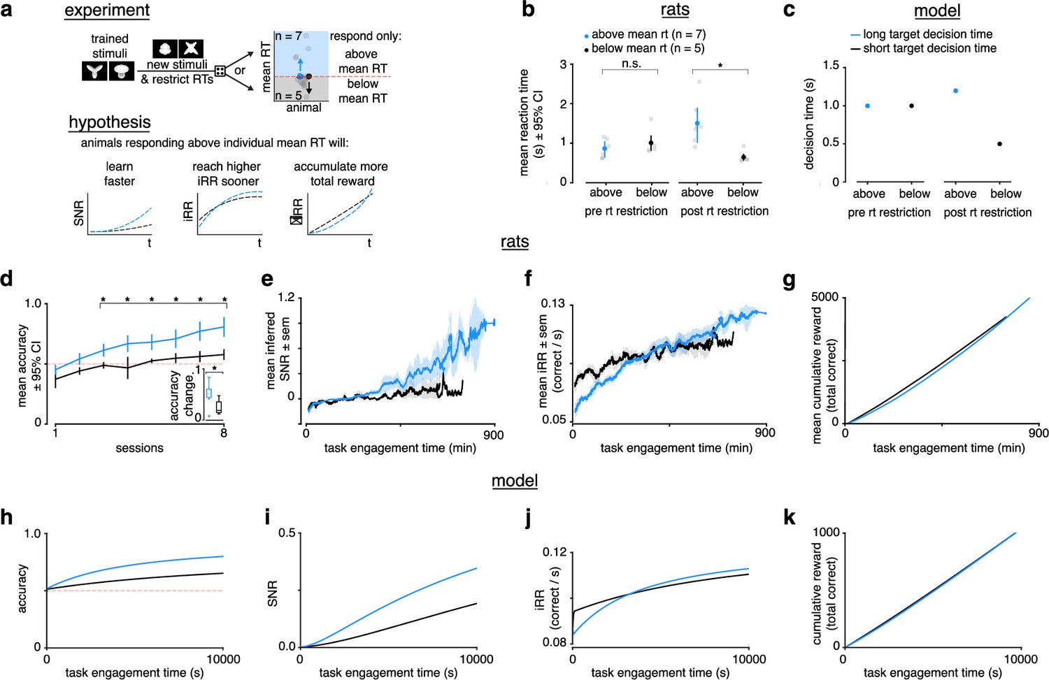
Longer reaction times lead to faster learning and higher instantaneous reward rates.
(a) Schematic of experiment and hypothesized results. Previously trained animals were randomly divided into two groups: could only respond above (blue, ) or below (black, ) their individual mean reaction times for the previously trained stimulus and the new stimulus. Subjects responding above their individual mean reaction times were predicted to learn faster, reach a higher instantaneous reward rate sooner and accumulate more total reward. (b) Mean and individual reaction times before and after the reaction time restriction in rats. The mean reaction time for subjects randomly chosen to respond above their individual mean reaction times (blue, ) was not significantly different to those randomly chosen to respond below their individual means (black, ) before the restriction (Wilcoxon rank-sum test p > 0.05), but were significant after the restriction (Wilcoxon rank-sum test p < 0.05). Errors represent 95% confidence intervals. (c) In the model a long (blue) and a short (black) target decision time were set through a control feedback loop on the threshold, with parameter . (d) Mean accuracy ±95% confidence interval across sessions for rats required to respond above (blue, ) or below (black, ) their individual mean reaction times for a previously trained stimulus. Both groups had initial accuracy below chance because rats assume a response mapping based on an internal assessment of similarity of new stimuli to previously trained stimuli. To counteract this tendency and ensure learning, we chose the response mapping for new stimuli that contradicted the rats’ mapping assumption, having the effect of below-chance accuracy at first. * denotes p < 0.05 in two-sample independent -test. Inset: accuracy change (slope of linear fit to accuracy across sessions to both groups, units: fraction per session). * denotes p < 0.05 in a Wilcoxon rank-sum test. (e) Mean inferred signal-to-noise ratio (SNR), (f) mean, and (g) mean cumulative reward across task engagement time for new stimulus pair for animals in each group. (h) Accuracy, (i) SNR, (j) , and (k) cumulative reward across task engagement time for long (blue) and short (black) target decision times in the linear drift-diffusion model (LDDM).
Figure 6 with 5 supplements
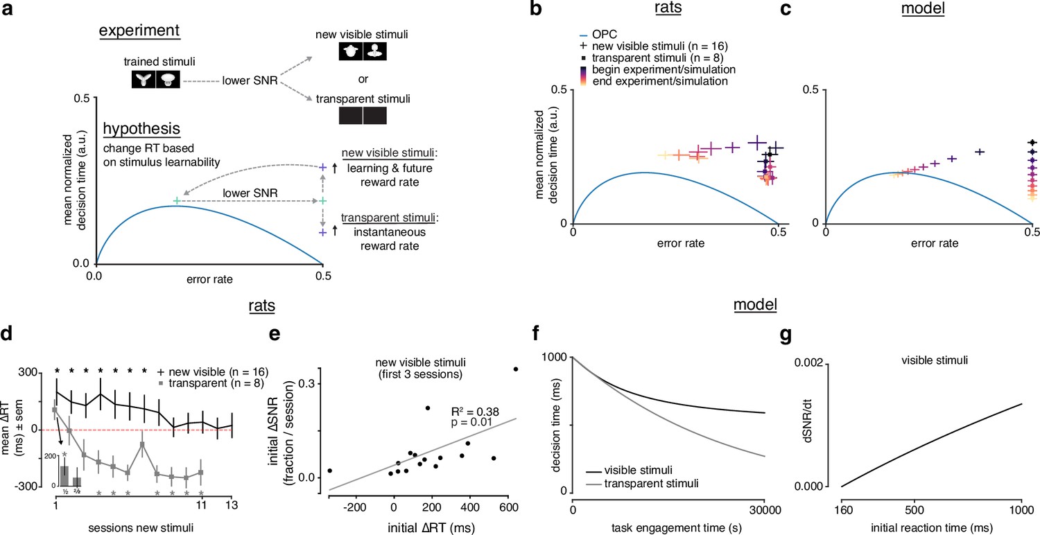
Rats choose reaction time based on stimulus learnability.
(a) Schematic of experiment: rats trained on stimulus pair 1 were presented with new visible stimulus pair 2 or transparent (alpha = 0, 0.1) stimuli. If rats change their reaction times based on stimulus learnability, they should increase their reaction times for the new visible stimuli to increase learning and future and decrease their reaction time to increase for the transparent stimuli. (b) Learning across normalized sessions in speed-accuracy space for new visible stimuli (, crosses) and transparent stimuli (, squares). Color map indicates time relative to start and end of the experiment. (c) -sensitive threshold model runs with ‘visible’ (crosses) and ‘transparent’ (squares) stimuli (modeled as containing some signal, and no signal) plotted in speed-accuracy space. The crosses are illustrative and do not reflect any uncertainty. Color map indicates time relative to start and end of simulation. (d) Mean change in reaction time across sessions for visible stimuli or transparent stimuli compared to previously known stimuli. Positive change means an increase relative to previous average. Inset: first and second half of first session for transparent stimuli. * denotes in permutation test. (e) Correlation between initial individual mean change in reaction time (quantity in d) and change in signal-to-noise ratio (SNR) (learning speed: slope of linear fit to SNR per session) for first three sessions with new visible stimuli. R2 and from linear regression in d. Error bars reflect standard error of the mean in b and d. (f) Decision time across time engagement time for visible and transparent stimuli runs in model simulation. (g) Instantaneous change in SNR () as a function of initial reaction time (decision time + non-decision time T0) in model simulation.
Figure 6—figure supplement 1

Reaction time analysis of transparent stimuli experiment.
(a) During transparent stimuli, the reaction time () minimum was relaxed to 0 ms to fully measure a possible shift in behavior. To be able to ascertain whether transparent stimuli led to a significant change in , the histogram of transparent stimuli (early [first two sessions]: purple, late [last two sessions]: yellow) sessions was compared to control sessions with visible stimuli (gray) with no minimum. Medians indicated with dashed lines. Kolmogorv-Smirnov two-sample tests over distributions found significant differences (). (b) Vincentized for transparent and control visible stimuli sessions with no minimum reaction time showed the early transparent sessions were slower than the control sessions, and the late sessions were faster across quantiles.
Figure 6—figure supplement 2
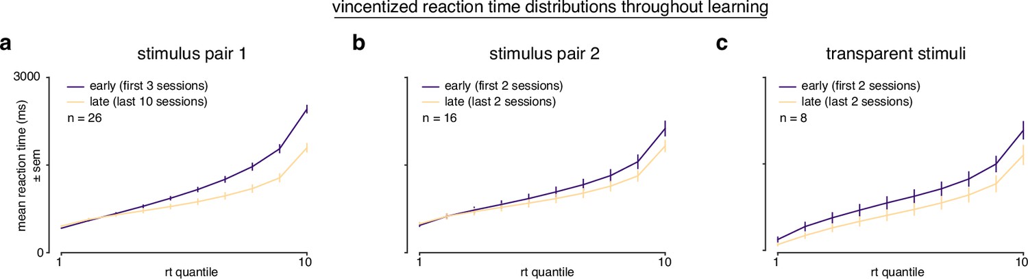
Vincentized reaction time distributions throughout learning.
(a) Vincentized reaction time distributions for subjects learning stimulus pair 1 (first 3 sessions, purple; last 10 asymptotic sessions, yellow). (b) Vincentized reaction time distributions for subjects learning stimulus pair 2 (first 2 sessions, purple; last 2 sessions, yellow). (b) Vincentized reaction time distributions for subjects learning transparent stimuli (first 2 sessions, purple; last 2 sessions, yellow).
Figure 6—figure supplement 3

Simple drift-diffusion model (DDM) + variable drift rate variability fits for transparent stimuli.
(a) The learning data from transparent stimuli were fit with a simple DDM + variable drift rate variability using the hierarchical DDM (HDDM) framework (Wiecki et al., 2013). Three learning phases were included: the last 500 trials with control visible stimuli, and the first 500 and the last trials with transparent stimuli. (a) We allowed drift rate, threshold, drift rate variability, and T0 to vary with learning phase. Drift rate decreased with transparent stimuli, remaining constant throughout. Threshold monotonically decreased with transparent stimuli. Drift rate variability appeared to decrease and stay constant with transparent stimuli, albeit at a value near 0. T0 appeared to decrease with transparent stimuli. p-Values were calculated as in Figure 4—figure supplement 2.
Figure 6—figure supplement 4
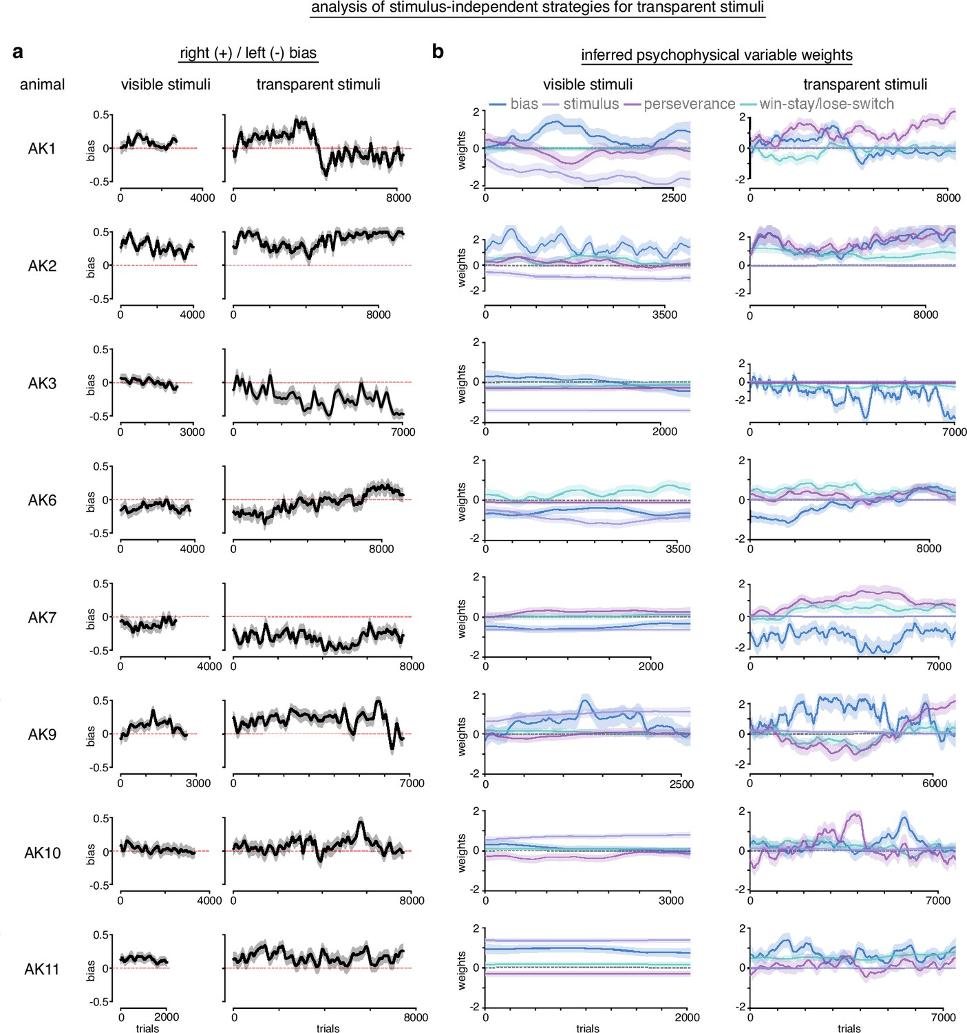
Analysis of stimulus-independent strategies for transparent stimuli.
In order to measure the extent of stimulus-independent strategies for transparent stimuli, we fit baseline sessions with visible stimuli and sessions with the transparent stimuli with PsyTrack, a flexible generalized linear model (GLM) package for measuring the weights of different inferred psychophysical variables (Roy et al., 2021). We fit our data with a model that included bias, win-stay/lose-switch (previous trial outcome), perseverance (previous trial choice), and the actual stimulus as potential explanatory variables for left/right choice behavior. (a) Measurement of bias across animals. Generally, bias and bias variability increased with transparent stimuli compared to visible stimuli. Although not uniform, animals tended to become more biased to the side that they were already biased during visible stimuli. (b) During visible stimuli, the stimulus had strong non-zero weights, indicating it influenced choice behavior. Stimulus has positive weights for some animals and negative for others because stimuli mappings were counterbalanced across animals. Win-stay/lose-switch and perseverance weights varied across animals during visible stimuli. Generally, these variables increased weights and variability during transparent stimuli, while the stimulus collapsed to a weight of 0 (as expected, given it was transparent). The weight of the bias variable was omitted for visual clarity as the actual bias was reported in a.
Figure 6—figure supplement 5

Post-error slowing during rat learning dynamics.
(a) Individual (gray) and mean (black) post-error slowing across first 15 sessions for animals. Post-error slowing was calculated by taking the difference between on trials with previous correct trials and previous error trials. A positive difference indicates post-error slowing. (b) Individual mean (gray) and population mean (black) post-error slowing for first 2 sessions of learning and last 2 sessions of learning for animals. A Wilcoxon signed-rank test found no significant difference in post-error slowing between the first 2 and last 2 sessions for every animal (p = 0.585). (c) Same as in a for rats, with the addition of 4 baseline sessions with stimulus pair 1 plus the 13 sessions while subjects were learning stimulus pair 2. (d) Same as in b but comparing the last 2 baseline sessions with stimulus pair 1 and the first 2 sessions learning stimulus pair 2. A Wilcoxon signed-rank test found no significant difference in post-error slowing when the animals started learning stimulus pair 2 (p = 0.255).
Figure 7
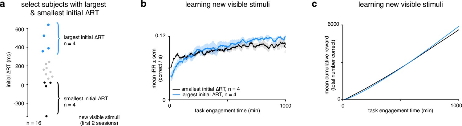
Rats that slowed down reaction times the most reached a higher instantaneous reward rate sooner and collected more reward.
(a) Schematic showing segregation of top 25% of subjects () with the largest initial ΔRTs for the new visible stimuli and the bottom 25% of subjects () with the smallest initial ΔRTs. Initial ΔRTs were calculated as an average of the first two sessions for all subjects. (b) Mean for subjects with largest and smallest mean changes in reaction time across task engagement time. (c) Mean cumulative reward over task engagement time for subjects as in b.
Tables
Table 1
Individual animal participation across behavioral experiments.
| Animal | Sex | Stimulus pair 1 | Stimulus pair 2 | Transparent stimuli | Stimulus pair 3 |
|---|---|---|---|---|---|
| AK1 | F | Size and rotation | Alpha = 0 | ||
| AK2 | F | Size and rotation | Alpha = 0.1 | ||
| AK3 | F | Size and rotation | Alpha = 0.0 | ||
| AK4 | F | Size and rotation | |||
| AK5 | F | Size and rotation | Alpha = 0.1 (excluded)‡ | ||
| AK6 | F | Size and rotation | Alpha = 0 | ||
| AK7 | F | Size and rotation | Alpha = 0 | ||
| AK8 | F | Size and rotation (excluded)* | |||
| AK9 | F | Size and rotation | Alpha = 0.1 | ||
| AK10 | F | Size and rotation | Alpha = 0.1 | ||
| AK11 | F | Size and rotation | Alpha = 0.0 | ||
| AK12 | F | Size and rotation | Alpha = 0.1 (excluded)‡ | ||
| AL1 | F | Size and rotation | Canonical only | (Excluded)§ | |
| AL2 | F | Size and rotation | Canonical only | Below | |
| AL3 | F | Size and rotation | Canonical only | Above | |
| AL4 | F | Size and rotation | Canonical only | Below (excluded) ¶ | |
| AL5 | F | Size and rotation | Canonical only | Below | |
| AL6 | F | Size and rotation | Canonical only | Below | |
| AL7 | F | Size and rotation | Canonical only | Below (excluded)¶ | |
| AL8 | F | Size and rotation | Canonical only | Above | |
| AL9 | F | Size and rotation | |||
| AL10 | F | Size and rotation | |||
| AL11 | F | Size and rotation | |||
| AL12 | F | Size and rotation (excluded)* | |||
| AL13 | F | Size and rotation | Canonical only | Above | |
| AL14 | F | Size and rotation | Canonical only | Below | |
| AL15 | F | Size and rotation | Canonical only | Above | |
| AL16 | F | Size and rotation | Canonical only | Above | |
| AM1 | F | Size and rotation† | Canonical only | Below (excluded)** | |
| AM2 | F | Size and rotation† | Canonical only | Below | |
| AM3 | F | Size and rotation† | Canonical only | Above | |
| AM4 | F | Size and rotation† | Canonical only | Above | |
| AM5 | F | Size and rotation† | |||
| AM6 | F | Size and rotation† | |||
| AM7 | F | Size and rotation† | |||
| AM8 | F | Size and rotation† | |||
| AN1 | F | Canonical only | |||
| AN2 | F | Canonical ony | |||
| AN3 | F | Canonical only | |||
| AN4 | F | Canonical only | |||
| AN5 | F | Canonical only | |||
| AN6 | F | Canonical only | |||
| AN7 | F | Canonical only | |||
| AN8 | F | Canonical only | |||
-
*
Failed to learn task.
-
†
Not included in initial learning experiment.
-
‡
Above chance for near-transparent stimuli.
-
§
Failed to learn previous stimuli.
-
¶
Not enough practice trials with reaction time restrictions.
-
**
Failed to learn stimuli with reaction time restrictions.
Additional files
Download links
A two-part list of links to download the article, or parts of the article, in various formats.
Downloads (link to download the article as PDF)
Open citations (links to open the citations from this article in various online reference manager services)
Cite this article (links to download the citations from this article in formats compatible with various reference manager tools)
Strategically managing learning during perceptual decision making
eLife 12:e64978.
https://doi.org/10.7554/eLife.64978


