Humans use forward thinking to exploit social controllability
- The Graduate School of Biomedical Sciences, Icahn School of Medicine at Mount Sinai, United States
- Nash Family Department of Neuroscience, Icahn School of Medicine at Mount Sinai, United States
- Department of Psychiatry, Icahn School of Medicine at Mount Sinai, United States
- Department of Biomedical Engineering, Ulsan National Institute of Science and Technology, Republic of Korea
- Austrian Institute of Technology, Austria
- School of Behavioral and Brain Sciences, The University of Texas at Dallas, United States
- Queen Square Institute of Neurology, University College London, United Kingdom
- Max Planck Institute for Biological Cybernetics, Germany
- University of Tübingen, Germany
Figures
Figure 1 with 1 supplement
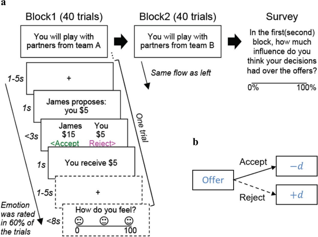
Experimental paradigm.
(a) Participants played a social exchange task based on the ultimatum game. There were two blocks: one ‘Controllable’ condition and one ‘Uncontrollable’ condition. Order of the conditions was counterbalanced across participants. Each block had 40 (fMRI sample) or 30 (online sample) trials. In each trial, participants needed to decide whether to accept or reject the split of $20 proposed by virtual members of a team. In the fMRI study, participants rated their emotions after their choice in 60% of the trials. Upon the completion of the game, participants rated their subjective beliefs about controllability for each block. (b) The schematic of the offers (the proposed participants’ portion of the split) generation under the Controllable condition. Under the Controllable condition, if participants accepted the offer at trial t, the next offer at trial t+1 decreased by d={0, 1, or 2} (1/3 chance each). If they rejected the offer, the next offer increased by d={0, 1, or 2} (1/3 chance for each option). Such contingency did not exist in the Uncontrollable condition where the offers were randomly drawn from a Gaussian distribution (μ=5, σ=1.2, rounded to the nearest integer, max=8, min=2) and participants’ behaviors had no influence on the future offers.
Figure 1—figure supplement 1
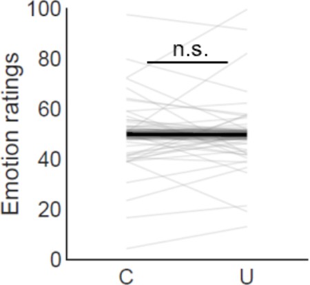
Emotion ratings.
In the fMRI version of the task, on 60% of the trials, we also measured participants’ emotional state (how do you feel?). Mean emotion ratings were not significantly different between the two conditions (meanC=49.9, meanU=49.7, t(47)=0.10, p=0.92). Each line represents a participant and the bold line represents the mean. C, controllable; fMRI, functional magnetic resonance imaging; n.s., not significant; U, Uncontrollable.
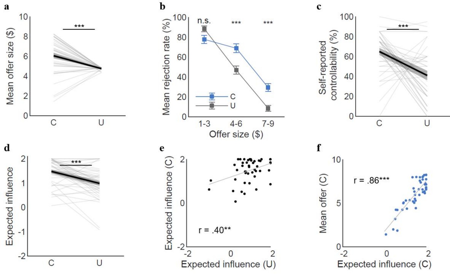
Figure 2 with 4 supplements
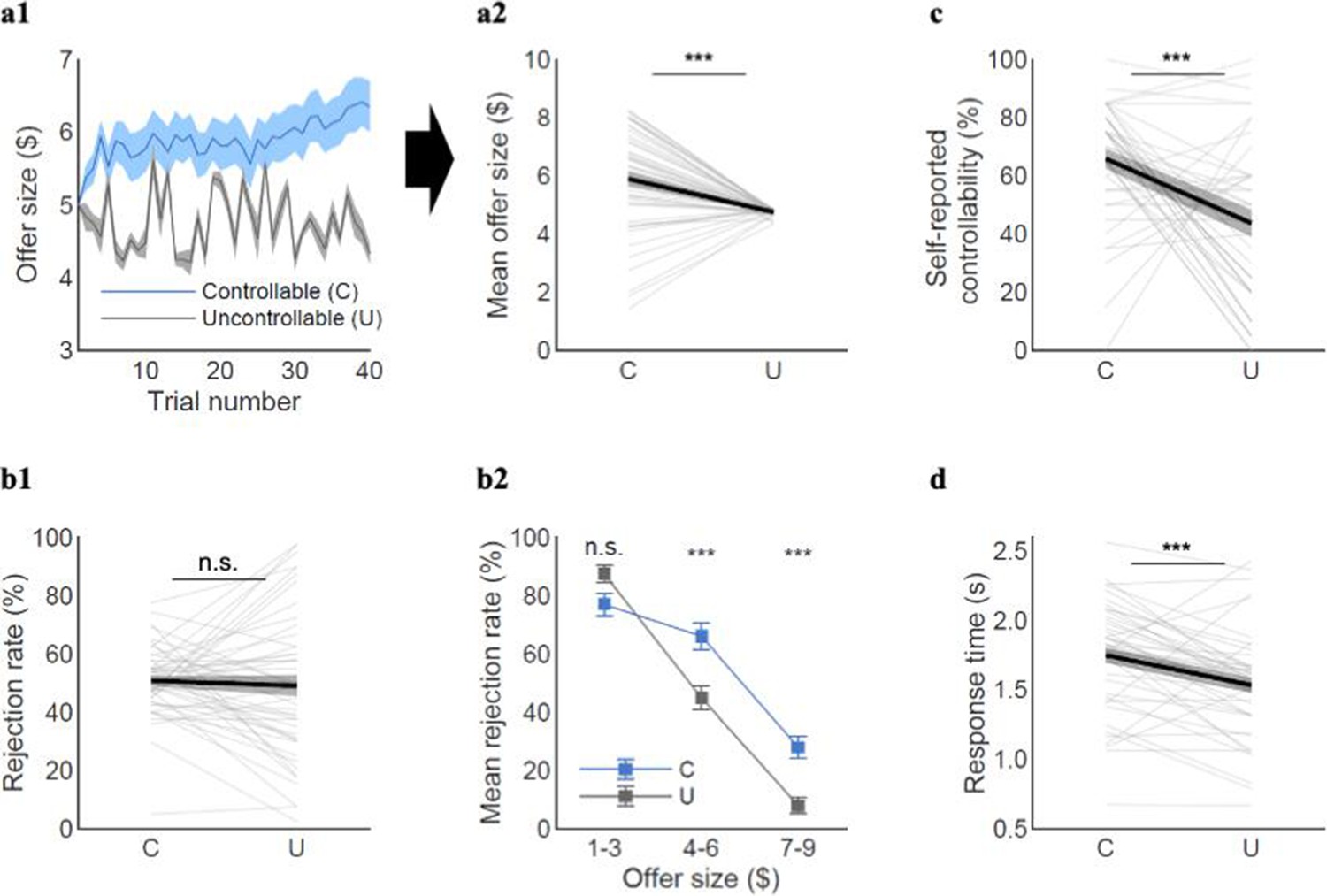
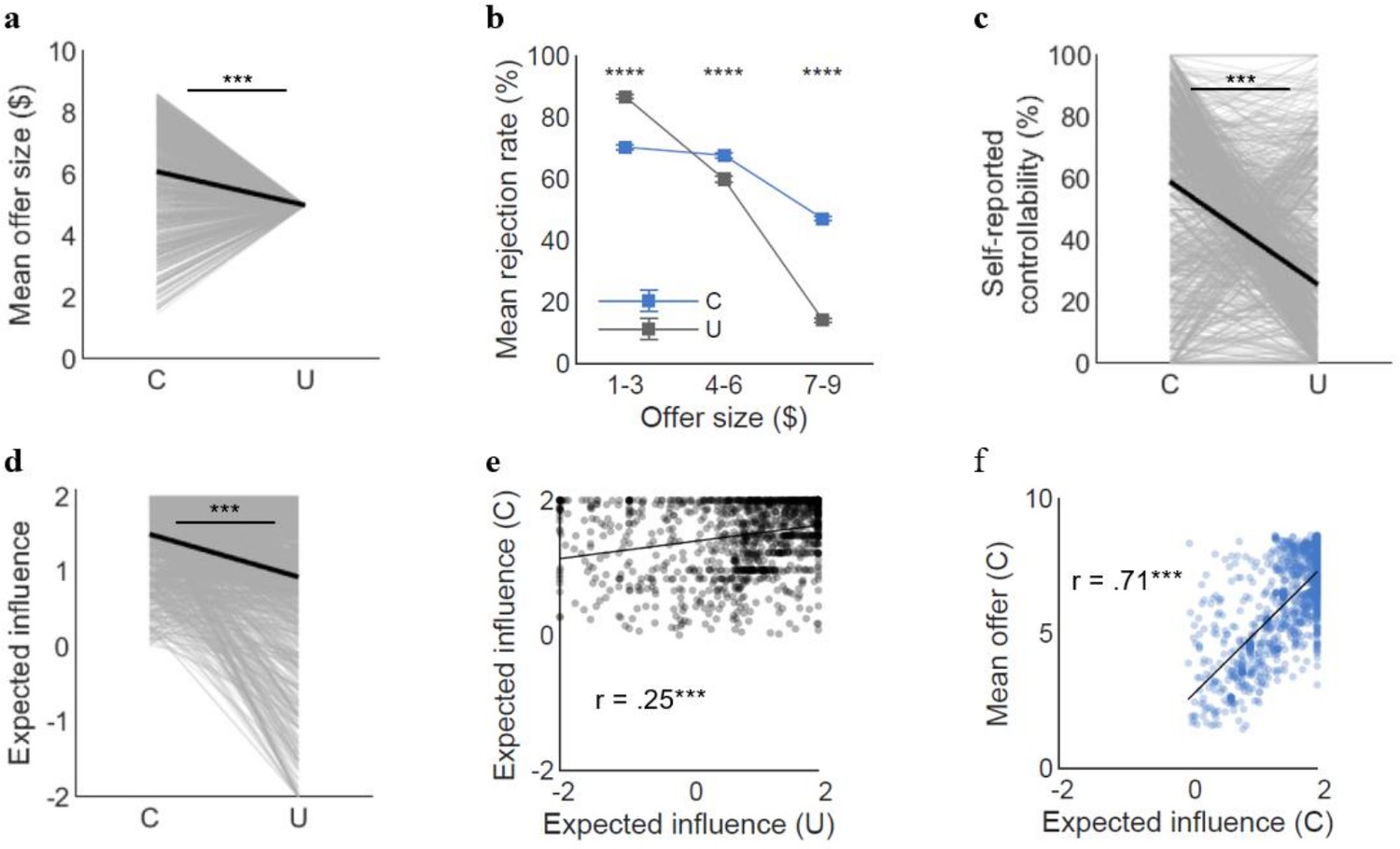
Model-agnostic behavioral results.
(a1) Participants raised the offers along the trials when they had control (Controllable), compared to when they had no control (Uncontrollable). (a2) The mean offer size was higher for the Controllable (C) than Uncontrollable (U) condition (meanC=5.9, meanU=4.8, t(47.45)=4.33, p<0.001). (b1) Overall rejection rates were not different between the two conditions (meanC=50.8%, meanU=49.1%, t(67.87)=0.43, p=0.67). (b2) However, participants were more likely to reject middle and high offers when they had control (low ($1–3): meanC=77%, meanU=87%, t(22)=–1.35, p=0.19; middle ($4–6): meanC=66%, meanU=45%, t(47)=5.41, p<0.001; high ($7–9): meanC=28%, meanU=8%, t(72.50)=4.00, p<0.001). Each offer bin for the Controllable in (b2) represents 23, 48, and 41 participants who were proposed the corresponding offers at least once, whereas each bin for the Uncontrollable represents all 48 participants. The t-test for each bin was conducted for those who had the corresponding offers for both conditions. (c) The self-reported controllability ratings were higher for the Controllable than Uncontrollable condition (meanC=65.9, meanU=43.7, t(74.55)=4.10, p<0.001; eight participants were excluded due to missing data). (d) Response times were longer for the Controllable than the Uncontrollable condition (meanC=1.75±0.38, meanU=1.53±0.38; paired t-test t(47)=4.34, p<0.001), suggesting that participants were likely to engage more deliberation during decision-making in the Controllable condition. A paired t-test was used for the rejection rates for low and middle offers and the self-reported controllability ratings. The t-statistics for the mean offer size, overall rejection rate, rejection rate for high offers, and self-reported controllability are from two-sample t-tests assuming unequal variance using Satterthwaite’s approximation according to the results of the F-tests for equal variance. Error bars and shades represent SEM; ***p<0.001; n.s. indicates not significant. For (a2, b1, c, d), each line represents a participant and each bold line represents the mean.
Figure 2—figure supplement 1
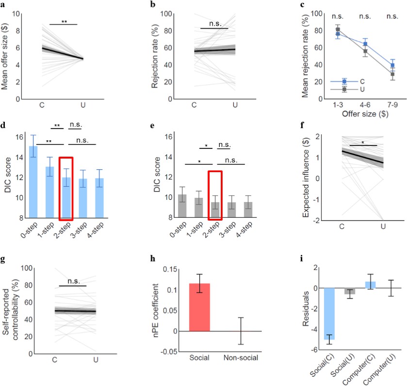
Behavioral results of a non-social controllability task.
To investigate whether our results are specific to the social domain, we ran another batch of the task in which 27 out of the 48 original participants were re-contacted with a 14- to 24-month temporal gap and played the same game with the instruction of ‘playing with computer’ instead of ‘playing with virtual human partners.’ Overall, we found choice patterns (a–f) similar to those in the social task, while the subjective states (i.e., self-reported controllability) (g) and the impact of the norm prediction error on the emotion ratings (Supplementary file 1) differed from the social task. (a) Similar to the results of the social task, offers (meanC=6.0, meanU=4.7, t(26.23)=3.03, p<0.01) were higher for the Controllable than the Uncontrollable. (b) Overall rejection rates (meanC=55.9%, meanU=58.1%, t(40.76)=–0.33, p=0.74) or (c) any of the binned rejection rates were not significantly different between the two conditions (paired t-test; low ($1–3): meanC=76%, meanU=81%, t(12)=1.54, p=0.15; middle ($4–6): meanC=64%, meanU=56%, t(26)=1.74, p=0.09; high ($7–9): meanC=39%, meanU=29%, t(19)=0.80, p=0.44). (d, e) The DIC scores showed a similar pattern to the social task, with the elbow point at the 2-step FT model for both conditions. Paired t-tests confirmed that the 2-step model’s DIC scores were significantly lower than the 0-step model (Controllable: t(26)=–3.16, p<0.01; Uncontrollable: t(26)=–2.38, p<0.05) and the 1-step model (Controllable: t(26)=–3.02, p<0.01; Uncontrollable: t(26)=–2.31, p<0.05), whereas the DIC scores were not significantly different between the 2-step model and the 3-step model (Controllable: t(26)=–1.23, p=0.23; Uncontrollable: t(26)=0.20, p=0.84) or the 4-step model (Controllable: t(26)=0.68, p=0.50; Uncontrollable: t(26)=–0.13, p=0.90). (f) Expected influence was significantly higher for the Controllable than the Uncontrollable condition (meanC=1.31, meanU=0.75, t(26)=2.54, p<0.05). (g) In contrast to the social task, self-reported controllability was not different between the two conditions when individuals played the game with a computer (meanC=62.7, meanU=56.9, t(25)=0.78, p=0.44). (h) To unpack the norm prediction error×social interaction effect in Supplementary file 1a, we used the regression coefficients from the original mixed-effect regression (‘emotion rating~ offer+norm prediction error+condition+task+task*(offer+norm prediction error+condition)+(1+offer+norm prediction error | subject)’) and calculated the residual, which should be explained by the differential impact of nPE between social and non-social tasks. Correlation coefficients between the residuals and nPE were plotted for each task condition (meanSocial=0.151, meanNon-social=0.005; SDSocial=0.023, SDNon-social=0.025). Note that the non-social task was coded as the reference group (0 for the group identifier) in our original regression. This result indicates that the impact of nPE was stronger in the social than in the non-social Computer task. Bars represent the mean of the coefficients and error bars represent the standard deviation. (i) To unpack the Controllable×social task interaction effect in Supplementary file 1a, similar to (h), we used the coefficients from the original mixed-effect regression (‘emotion rating~ offer+norm prediction error+condition+task+task*(offer+norm prediction error+condition)+(1+offer+norm prediction error | subject)’) and calculated the residual by each condition and task as shown in the figure (meanSocial(C)=–5.00, meanSocial(U)=–0.58, meanComputer(C)=0.63, mean Computer(U)=0.00; SEMSocial(C)=0.46, SEMSocial(U)=0.43, SEMComputer(C)=0.72, SEMComputer(U)=0.77). Bars represent the mean of the coefficients and error bars represent SEM. Note that the non-social task and the Uncontrollable condition were coded as the reference group (0 for the group identifiers) in the regression. These results show that the emotion ratings were lower in the Controllable social context compared to the non-social as well as the Uncontrollable social context. We speculate that exerting control over other people—compared to not needing to exert control over other people or playing with computer partners—might be more effortful (as shown by our RT results). Intentionally decreasing other people’s portion of money might also induce a sense of guilt. Satterthwaite’s approximation was used for the effective degrees of freedom for t-test with unequal variance. The variance significantly differed for the offer and the overall rejection rates. Error bars and shades represent SEM. *p<0.05; **p<0.01; n.s. indicates not significant. For (a, b, f, g), each line represents a participant and each bold line represents the mean. DIC, Draper’s Information Criteria; FT, forward thinking.
Figure 2—figure supplement 2
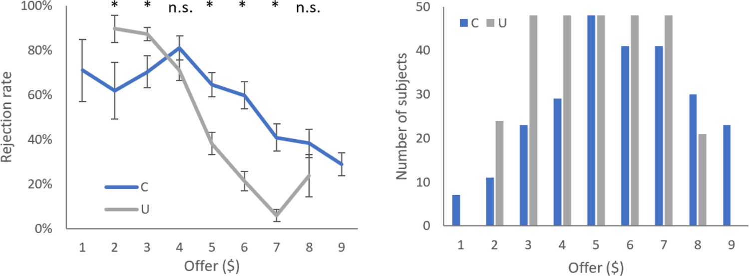
Rejection rates as a function of offer size.
We reported and displayed the binned rejection rates mainly for two reasons: (1) It had a better matched subsample size for each bin and (2) the range of the offers were unmatched unintentionally for the fMRI sample ($1–9 for the Controllable condition; $2–8 for the Uncontrollable condition). (a) Rejection rates by each offer size show by and large consistent pattern with the binned results. (b) Participants distribution is depicted by each offer size. Note that a mixed-effect logistic regression, a statistically more stringent analysis, still shows consistent results with the binned results (Supplementary file 1). Error bars represent SEM; *p<0.05; C, controllable; fMRI, functional magnetic resonance imaging; n.s., not significant; U, Uncontrollable.
Figure 2—figure supplement 3
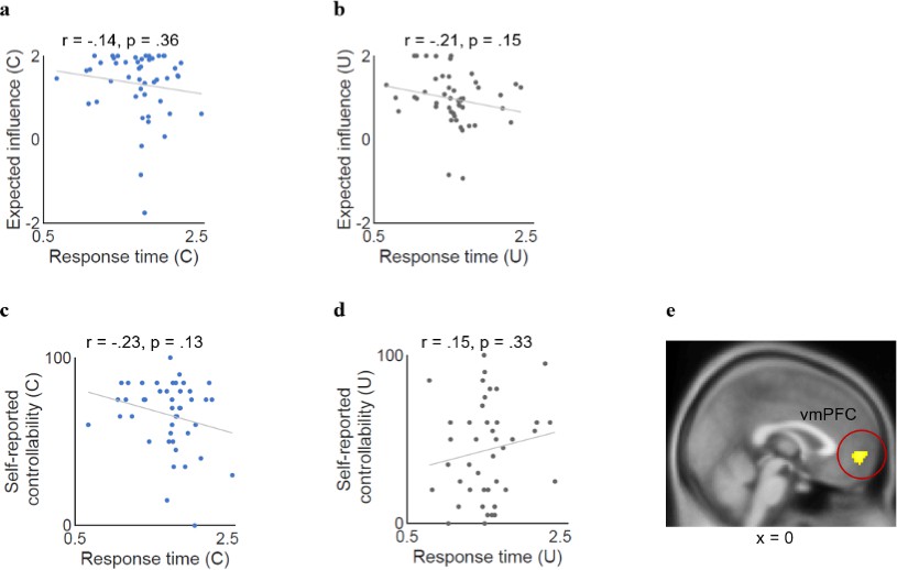
Response time.
For neither condition, response times showed correlation (a, b) with expected influence, or (c, d) with self-reported controllability. Each dot represents a participant. (e) We also conducted fMRI analyses to include trial-by-trial RT as the first parametric regressor followed by our main parametric regressor (chosen values) in the original GLM. We did not find any significant neural activation in relation to the response time that survived the threshold of PFDR<0.05. However, consistent with the result from the GLM without response times, the vmPFC chosen value signals were still significant at PFDR<0.05 and k>50 after controlling for any potential RT effects (peak coordinate [0, 54, –2]). Error bars and shades represent EM. *p<0.05; **p<0.01; n.s. indicates not significant. For (a–d), each dot represents a participant. C, controllable; fMRI, functional magnetic resonance imaging; n.s., not significant; U, Uncontrollable; vmPFC, ventromedial prefrontal cortex.
Figure 2—figure supplement 4
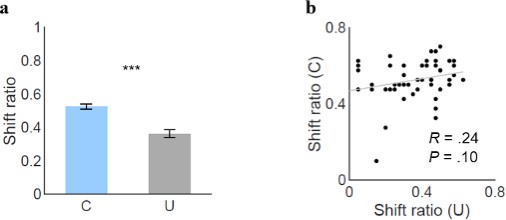
Shift ratio.
To examine whether participants behaved in a more habitual way in the Controllable condition, we analyzed the shift ratio of both conditions (i.e., the number of the trials where the choice was shifted from the previous trial divided by the total number of the trials). (a) We found that shift ratio was higher for the Controllable than the Uncontrollable condition (meanC=52.5%, meanU=36.2%, t(47)=6.62, p<0.001). (b) Shift ratio was not significantly correlated between the two conditions (r=0.24, p=0.10). Together with the RT analysis (Figure 2d), these results suggest that participants were less habitual and more deliberative in the Controllable condition.
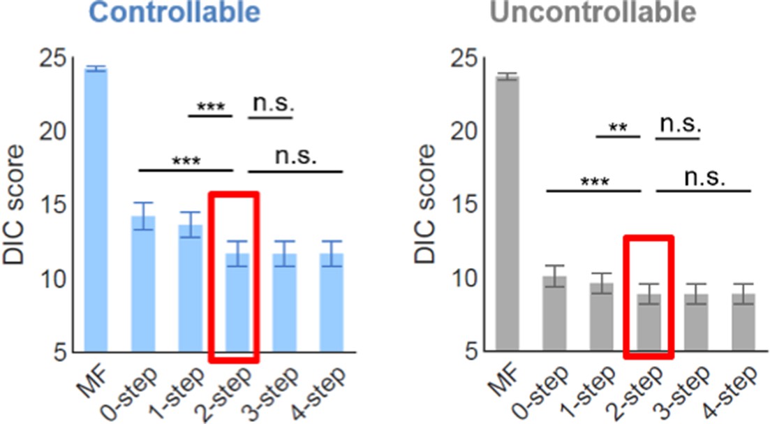
Figure 3 with 5 supplements

Computational modeling of social controllability.
(a) The figure depicts how individuals’ simulated value of the offers evolves contingent upon the choices along the future steps under the Controllable condition. Future simulation was assumed to be deterministic (only one path is simulated instead of all paths being visited in a probabilistic manner). The solid and thicker arrows represent an example of a simulated path. To examine how many steps along the temporal horizon participants might simulate to exert control, we tested the candidate models considering from zero to four steps of the future horizon. (b) For both the Controllable and Uncontrollable conditions, the forward thinking (FT) models better explained participants’ behavior than the 0-step model. The 2-step FT model was selected for further analyses, because the improvement in the DIC score (Draper’s Information Criteria; Draper, 1995) was marginal for the models including further simulations (paired t-test comparing 2-step FT model with (i) 0-step Controllable: t(47)=–4.45, p<0.0001, Uncontrollable: t(47)=–4.21, p<0.001; (ii) 1-step Controllable: t(47)=–4.41, p<0.0001, Uncontrollable: t(47)=–3.01, p<0.001; (iii) 3-step Controllable: t(47)=0.39, p=0.70, Uncontrollable: t(47)=–0.04, p=0.97; (iv) 4-step Controllable: t(47)=0.06, p=0.95, Uncontrollable: t(47)=–0.12, p=0.91). (c) The choices predicted by the 2-step FT model were matched with individuals’ actual choices with an average accuracy rate of 83.7% for the Controllable and 90.1% for the Uncontrollable. Each bold black line represents mean accuracy rate. (d) The levels of expected influence drawn from the 2-step FT model were higher for the Controllable than the Uncontrollable (meanC=1.33, meanU=0.98, t(47)=2.90, p<0.01). Each line represents a participant and each bold line represents the mean. (e) The expected influence was positively correlated between the Controllable and the Uncontrollable conditions (R=0.30, p<0.05). (f) The self-reported controllability was not significantly correlated between the conditions (R=–0.18, p=0.26). (g) Under the Controllable condition, expected influence correlated with mean offers (R=0.78, p<<0.0001). Each dot represents a participant. Error bars and shades represent SEM; ****p<0.0001; ***p<0.001; **p<0.01; *p<0.05. C, controllable; U, Uncontrollable.
Figure 3—figure supplement 1
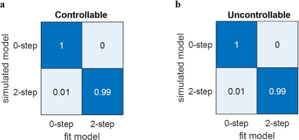
Model recovery analyses.
To examine whether our task design is sensitive enough to distinguish the models, we simulated each model where we fixed the inverse temperature at 10 to reduce noise and constrained the delta to be positive (between [0 2], inclusive) to make it similar to the actual empirical behavior we found. Other parameters were randomly sampled within the originally assumed range. We ran 100 iterations of simulation where in each iteration, behavioral choices of 48 individuals (which is equal to our fMRI sample size) were simulated. Next, we fit each model to each model’s simulated data where all the settings were identical to the original settings. Consistent with our original method, we calculated average DIC scores and determined the winning model of each iteration. In this set of new analysis, we focused on two distinct types of models in our model space, namely, no FT (0-step) and FT (2-step) models. Note that we chose the 2-step FT model as a representative of the FT models due to both its simplicity (i.e., per Occam’s razor) and the similarity amongst the FT models. The numbers represent p(fit model | simulated model), the probability that the data simulated with each model on the y-axis are best fit by each model on the x-axis. The models were well recovered for both (a) the Controllable and (b) the Uncontrollable conditions. DIC, Draper’s Information Criteria; fMRI, functional magnetic resonance imaging; FT, forward thinking.
Figure 3—figure supplement 2
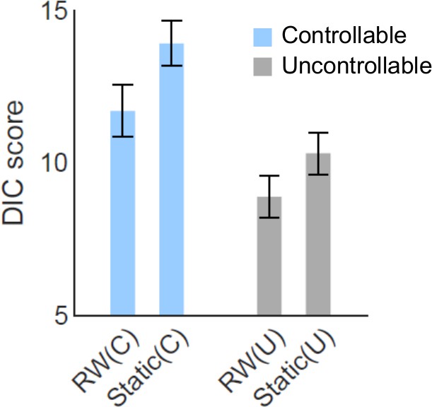
Adaptive norm learning versus static norm models.
We have examined an alternative 2-step FT model that has a static norm throughout all trials within each condition. The DIC scores of the alternative model (static) were higher than the 2-step FT model incorporating Rescorla-Wagner (RW) learning in both conditions (smaller DIC score indicates a better model fit). This result suggests that the adaptive norm learning model still offers a better account for behavior than the static norm model. Error bars represent SEM. DIC, Draper’s Information Criteria; FT, forward thinking.
Figure 3—figure supplement 3
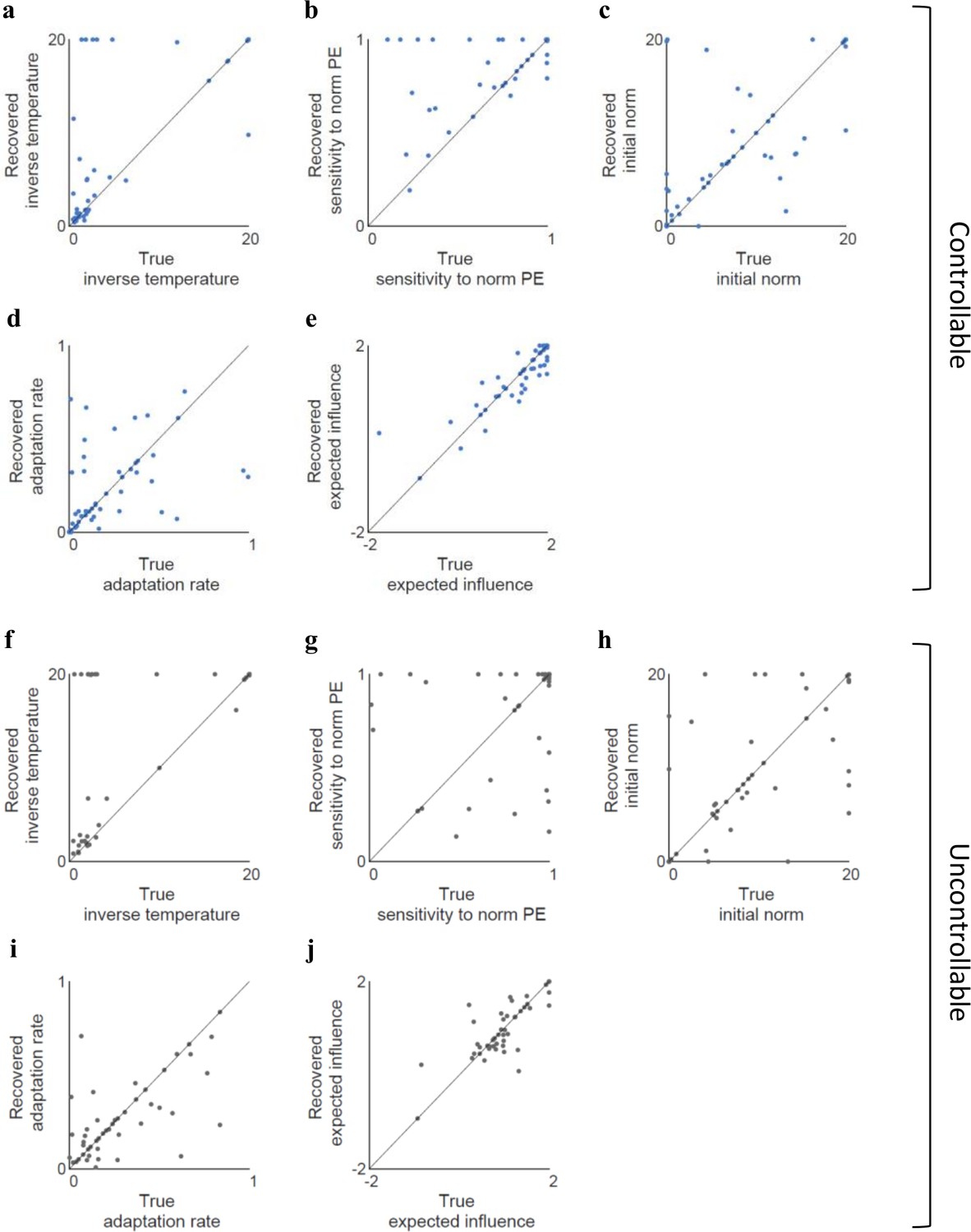
Parameter recovery.
To assess the estimation quality of the 2-step FT model, we tested whether the parameters were precisely recovered for each condition. We set the parameter estimates from the model as the true parameters and then by using the same model, we generated individuals’ response data under the actual offers and the true parameters. Under the Controllable condition (a–e), all parameters were well identified: (a) inverse temperature (β) (r=0.77, p<10–9), (b) sensitivity to norm PE (α) (r=0.57, p<10–4), (c) initial norm (μ) (r=0.66, p<10–6), (d) adaptation rate (ε) (r=0.39, P<0.01), and (e) expected influence (δ) (r=0.88, P<10–15). Under the Uncontrollable condition as well (f-j), all parameters were well identified: (f) inverse temperature (β) (r=0.69, p<10–7), (g) sensitivity to norm PE (α) (r=0.33, p<0.05), (h) initial norm (μ) (r=0.62, p<10–5), (i) adaptation rate (ε) (r=0.66, p<10–6), and (j) expected influence (δ) (r=0.79, p<10–10). Each dot represents an individual. FT, forward thinking.
Figure 3—figure supplement 4
fMRI sample: results without those who had negative deltas.
We initially allowed the delta parameter to be in a range of –2 to 2, because in the Uncontrollable condition, due to its randomly sampled offers, subsequent offers could drop after a rejection and increase after an acceptance (i.e., opposite direction from the Controllable condition). Here, we show that all behavioral results still held without those who had negative deltas under the Controllable condition. Specifically, there were statistically significant differences between the two conditions in (a) offer size (t(44)=5.05, p<0.001), (b) rejection rates for the middle (t(44)=5.33, p<0.001) and high offers (t(38)=4.68, p<0.001), (c) self-reported controllability (t(36)=3.67, p<0.001), and (d) expected influence (t(44)=5.14, p<0.001). Furthermore, (e) expected influence was positively correlated between the two conditions (r=0.40, p<0.01), and (f) particularly, expected influence under the Controllable condition was positively correlated with mean offers (R=0.86, p<0.001). Error bars and shades represent SEM. **p<0.01; ***p<0.001; n.s. indicates not significant. For (a, c, d), each line represents a participant and each bold line represents the mean. For (e f), each dot represents a participant. fMRI, functional magnetic resonance imaging.
Figure 3—figure supplement 5
Comparison with model-free (MF) learning.
We compared our set of models with classic MF learning in which we assumed that the value of the offer given the chosen action () updates the reward prediction error (RPE), with a learning rate of () after the reward () and the next offer () is observed. The actual rewards here consist of the utility of the immediate reward and the discounted value of the observed subsequent offer where the offer value assumes deterministic greedy choice at the corresponding trial, consistent with the FT valuation. The reward utility was based on the RW norm adaptation and the inequity aversion model same as the other models. , the difference in values between accepting and rejecting, was entered to the softmax function in the same way as the other models. The DIC scores indicate that the FT models significantly fit better than the MF learning does for both conditions. DIC, Draper’s Information Criteria; FT, forward thinking; RW, Rescorla-Wagner.
Figure 4 with 4 supplements
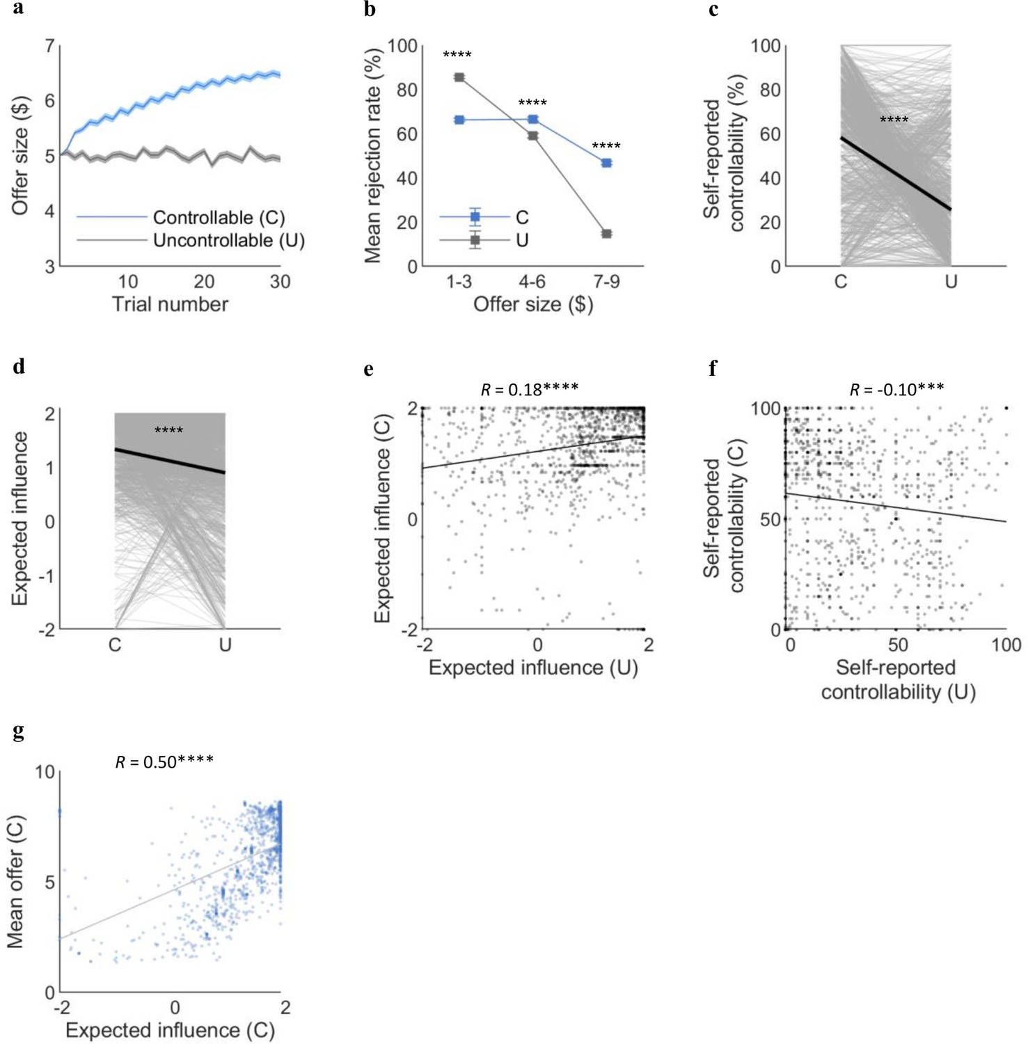
Replication of the behavioral and computational results in an independent large online sample (n=1342).
(a) Online participants successfully increased the offer under the Controllable condition as fMRI participants did (meanC=6.0, meanU=5.0, t(1,341)=20.29, p<<0.0001). (b) Rejection rates binned by offer sizes differed between the two conditions in the online sample (low ($1–3): meanC=66%, meanU=86%, t(741.54)=–12.28, p<<0.0001; middle ($4–6): meanC=67%, meanU=59%, t(2,606)=5.96, p<<0.0001; high ($7–9): meanC=47%, meanU=15%, t(1,925)=31.67, p<<0.0001). (c) Online participants reported higher self-reported controllability for the Controllable than Uncontrollable (meanC=58.3, meanU=25.6, t(2,579)=27.93, p<<0.0001). (d) Consistent with the fMRI sample, expected influence was higher for the Controllable than the Uncontrollable for the online sample (meanC=1.34, meanU=0.90, t(1,341)=12.97, p<<0.0001). (e) The expected influence was correlated between the two conditions (r=0.18, p<<0.0001). (f) The self-reported controllability showed negative correlation between the two conditions for the online sample (r=–0.10, p<0.001). (g) The significant correlation between expected influence and mean offers under the Controllable was replicated in the online sample (r=0.50, p<<0.0001). Each dot represents a participant. The t-statistics for the mean offer size, binned rejection rate, and self-reported controllability are from two-sample t-tests assuming unequal variance using Satterthwaite’s approximation according to the results of F-tests for equal variance. Error bars and shades represent SEM. For (c, d), each line represents a participant and each bold line represents the mean. C, controllable; U, Uncontrollable.
Figure 4—figure supplement 1
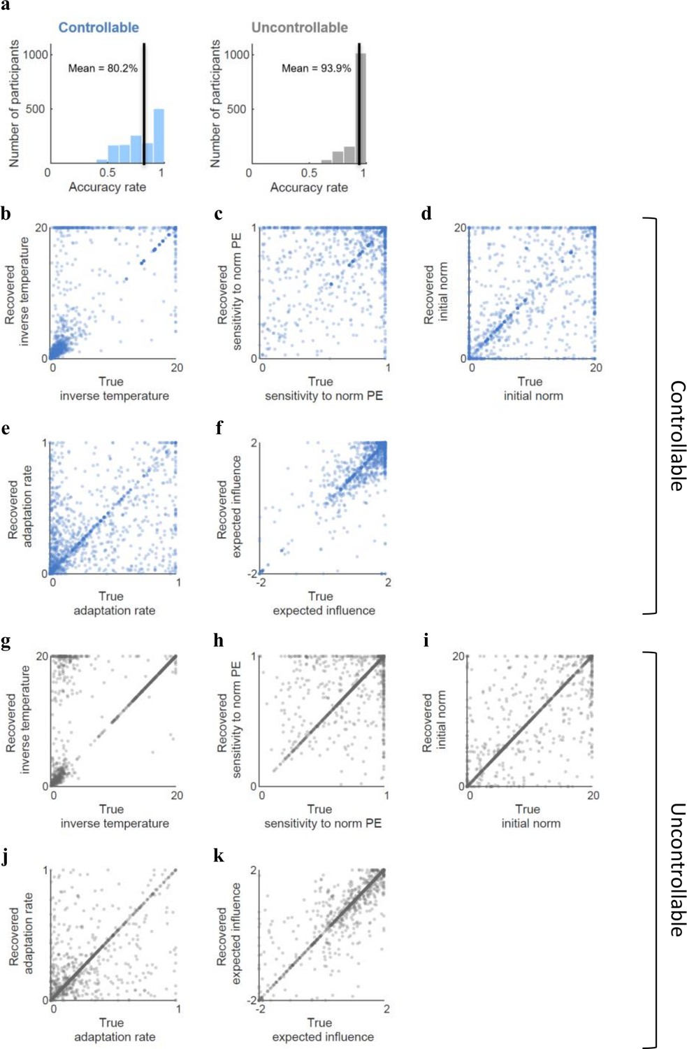
Model accuracy and parameter recovery for the online sample.
(a) The 2-step FT model’s prediction of choices was accurate for 80.2% of the trials on average for the Controllable, and 93.9% for the Uncontrollable. Each bold black line represents mean accuracy rate. (b–k) We recovered the parameters from the 2-step FT model for the online sample in the same way as we did for the fMRI sample. Under the Controllable condition, all parameters were well identified: (b) inverse temperature (β) (r=0.79, p<10–289), (c) sensitivity to norm PE (α) (r=0.39, p<10–49), (d) initial norm (μ) (r=0.60, p<10–136), (e) adaptation rate (ε) (r=0.48, p<10–77), and (f) expected influence (δ) (r=0.87, p<10–325). Under the Uncontrollable condition as well, all parameters were well identified: (g) inverse temperature (β) (r=0.74, p<10–235), (h) sensitivity to norm PE (α) (r=0.60, p<10–130), (i) initial norm (μ) (r=0.82, p<10–325), (j) adaptation rate (ε) (r=0.68, p<10–182), and (k) expected influence (δ) (r=0.90, p<10–325). Each dot represents an individual. fMRI, functional magnetic resonance imaging; FT, forward thinking.
Figure 4—figure supplement 2
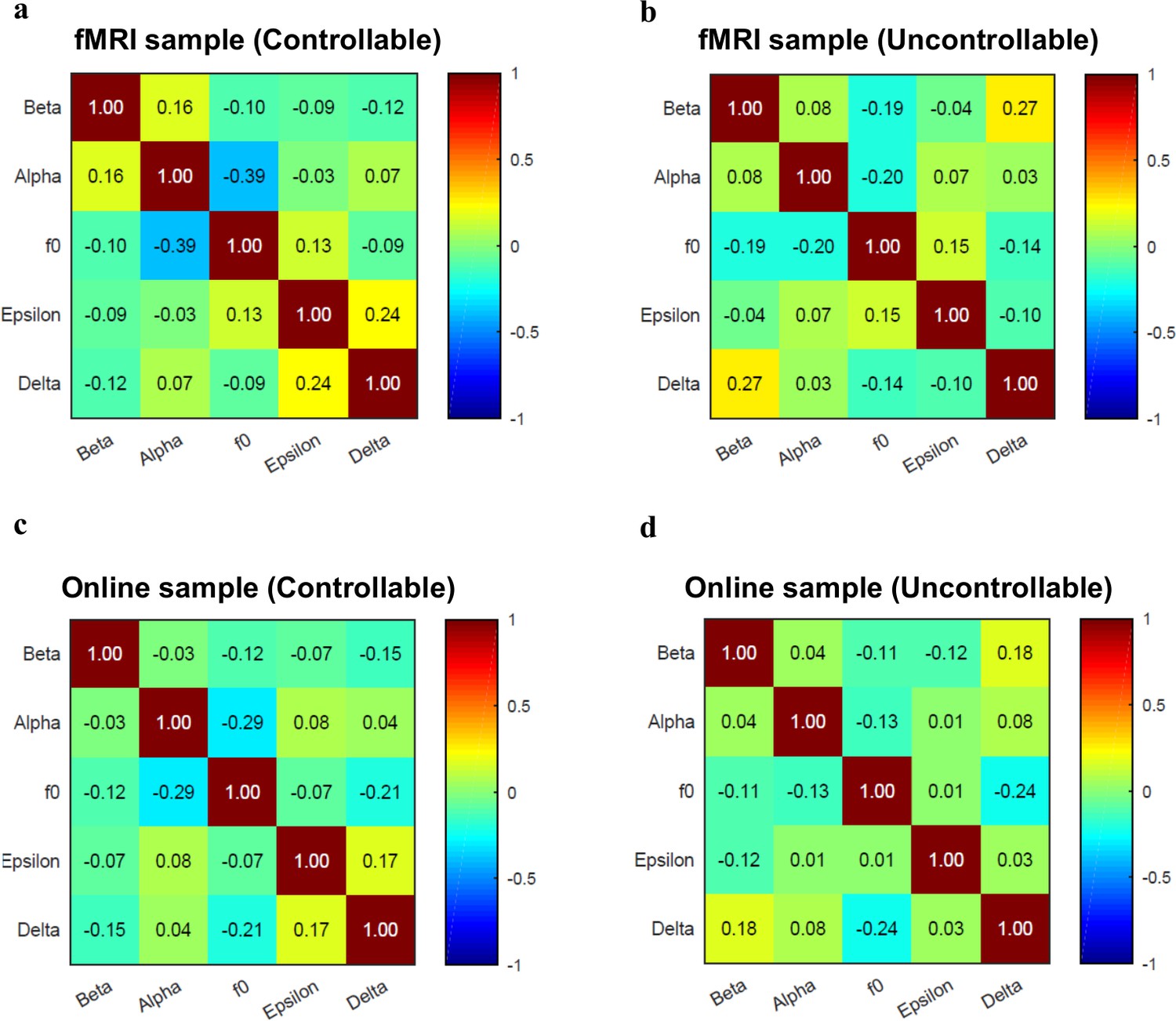
Cross-parameter correlations.
The numbers in the matrix denote Pearson’s correlation coefficients. The parameters did not have high correlations in general. The alpha (sensitivity to norm prediction error) and the f0 (initial norm) was moderately negatively correlated (r=–0.39) under the Controllable condition for the fMRI sample, but they still were recoverable (alpha: r=0.57, p<10–4, f0: r=0.66, p<10–6; see Figure 3—figure supplement 3b,c). fMRI, functional magnetic resonance imaging.
Figure 4—figure supplement 3
Online sample: results without those who had negative deltas.
All behavioral results still held without the individuals who had negative deltas. Specifically, there were significant differences between the two conditions in (a) offer size (t(1,265)=22.94, p<0.001), (b) rejection rates for the middle (t(1,265)=10.23, p<0.001) and high offers (t(934)=31.40, p<0.001), (c) self-reported controllability (t(1,265)=26.23, p<0.001), and (d) expected influence (t(1,265)=19.54, p<0.001). (e) Expected influence was positively correlated between the two conditions (r=0.25, p<0.001), and (f) particularly, expected influence under the Controllable condition was positively correlated with mean offers (r=0.71, p<0.001). Error bars and shades represent SEM. ***p<0.001. For (a, c, d), each line represents a participant and each bold line represents the mean. For (e, f), each dot represents an individual. C, Controllable; U, Uncontrollable.
Figure 4—figure supplement 4
Correlations between expected influence and self-reported controllability for each condition and each sample.
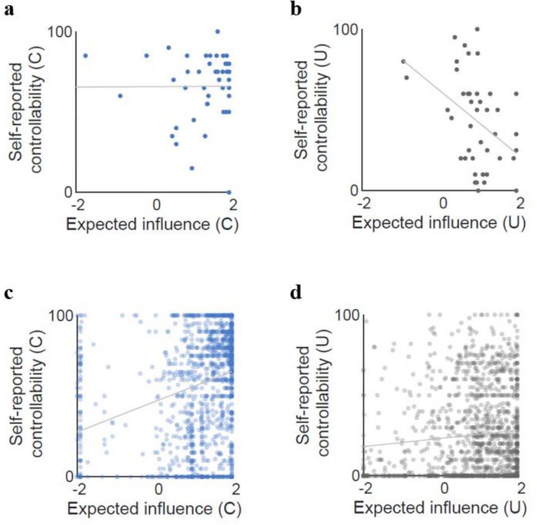
(a, b) For the fMRI sample, expected influence and self-reported controllability were not correlated under the Controllable condition (r=0.00, p=0.98), but negatively correlated under the Uncontrollable condition (r=–0.43, p<0.01). (c, d) For the online sample, self-reported controllability was correlated with expected influence for both the Controllable (r=0.27, p<<0.0001) and the Uncontrollable conditions (r=0.10, p<0.001). Here, expected influence captures an individual’s estimation of controllability on an objective scale (in dollars), whereas self-reported belief reflects a person’s sense of controllability on a subjective scale (0–100%). Despite the result from the fMRI sample, it would be unrealistic that the practical mental estimation of controllability and the high-level belief about it are completely dissociated. Indeed, the larger online sample showed a weak but positive correlation between the two measures. Although quantitative measures of ‘mentally simulated’ controllability are absent, the existing literature also supports the significant connection between ‘actual’ controllability and perceived controllability (Guinote, 2017; Lachman and Weaver, 1998). Based on such premise, further studies are needed to assess the structure of their relationship (i.e., to what degree they are processed hierarchically and in parallel) and thus to better understand the connection and discrepancy of the two systems—exploitation of controllability and the construction of sense of control. Each dot represents an individual. C, controllable; fMRI, functional magnetic resonance imaging; U, Uncontrollable.
Figure 5 with 5 supplements
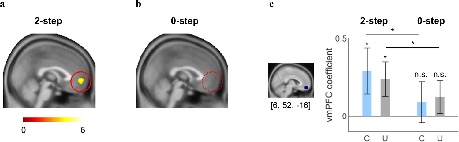
The ventromedial prefrontal cortex (vmPFC) computes projected summed choice values in exerting social controllability.
(a) The vmPFC parametrically tracked mentally simulated values of the chosen actions drawn from the 2-step forward thinking (FT) model in both conditions (PFDR<0.05, k>50). (b) No activation was found in the brain including the vmPFC in relation with the value signals estimated from the 0-step model at a more liberal threshold (p<0.005, uncorrected, k>50). (c) The vmPFC ROI coefficients for the 2-step FT’s value estimates were significantly greater than 0 for both the Controllable and Uncontrollable conditions (Controllable: meanC=0.29, t(47)=1.96, p<0.05 (one-tailed); Uncontrollable: meanU=0.24, t(47)=2.14, p<0.05 (one-tailed)) whereas the coefficients from the same ROI for 0-step’s value estimates were not significant for either condition (Controllable: meanC=0.09, t(46)=0.69, p=0.25 (one-tailed); Uncontrollable: meanU=0.12, t(46)=1.17, p=0.12 (one-tailed)). The vmPFC coefficients were significantly higher under the 2-step model than the 0-step model for both the Controllable and Uncontrollable conditions (Controllable: t(46)=1.81, p<0.05 (one-tailed); Uncontrollable: t(46)=2.04, p<0.05 (one-tailed)). The coefficients were extracted from an 8-mm-radius sphere centered at [6, 52, −16] based on a meta-analysis study that assessed neural signatures in the ultimatum game (Feng et al., 2015). Error bars represent SEM; *p<0.05; n.s. indicates not significant. C, Controllable; ROI, region-of-interest; U, Uncontrollable.
Figure 5—figure supplement 1
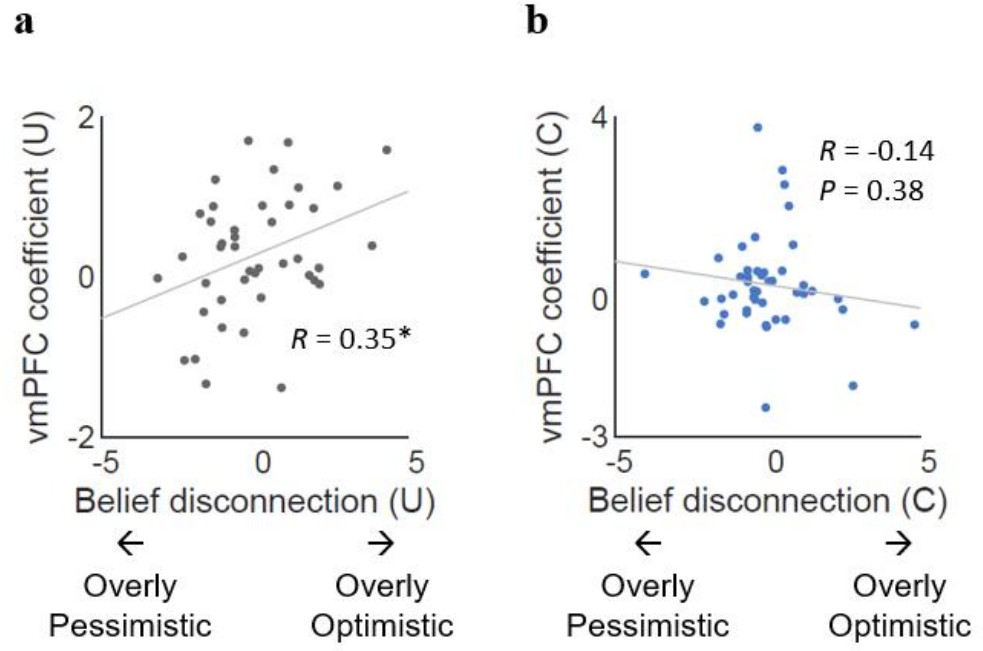
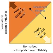
Neural encoding of value in the vmPFC is associated with behavior-belief disconnect under the Uncontrollable condition.
(a) The disconnect between self-reported controllability (belief) and expected influence (exploited controllability) was calculated by subtracting the normalized expected influence from the normalized self-reported belief. Under the Uncontrollable condition, this ‘belief disconnect’ was positively correlated with beta coefficient extracted from the vmPFC ROI (r=0.35, p<0.05). (b) Under the Controllable condition, belief disconnect and beta coefficient extracted from the vmPFC ROI were not significantly correlated (r=–0.14, p=0.38). *p<0.05; n.s. indicates not significant. Each dot represents a participant. C, Controllable; ROI, region-of-interest; U, Uncontrollable; vmPFC, ventromedial prefrontal cortex.
Figure 5—figure supplement 2
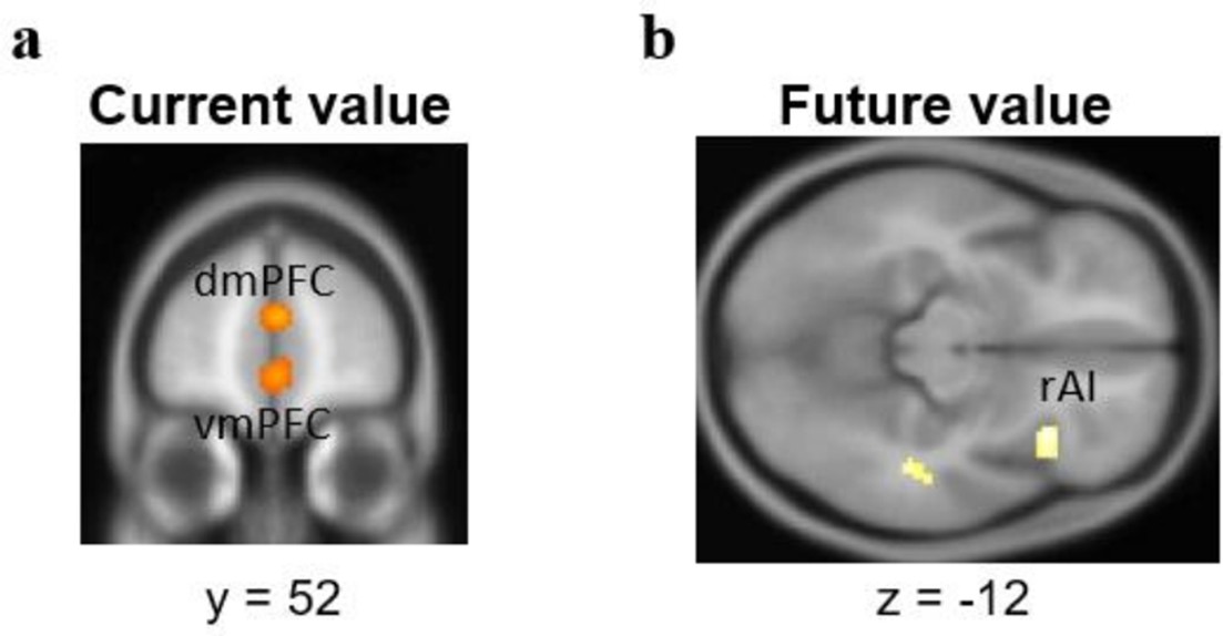
Current and future value signals.
We examined whether the current and future value terms under the same (2-step FT) model might be encoded by different neural substrates using a new set of GLMs with both the current and the future values without orthogonalization. We found that (a) the current value-alone signal was encoded in the vmPFC (peak voxel [2, 52, −4]) and the dmPFC ([2, 50, 18]), and (b) the future value-alone signal was tracked by the right anterior insula ([34, 22, −12]), at the threshold of p<0.001, uncorrected. Although these results did not survive the more stringent threshold applied to the main results (PFDR<0.05, k>50), all survived the small volume correction at PSVC<0.05. The results here are displayed at p<0.005, uncorrected, k>15. Together with our main result, these results indicate that the vmPFC encodes both current and total values estimated from the 2-step FT model; and that current and future value signals also had distinct neural substrates (dmPFC and insula). FT, forward thinking; vmPFC, ventromedial prefrontal cortex.
Figure 5—figure supplement 3
GLM comparison at the neural level.
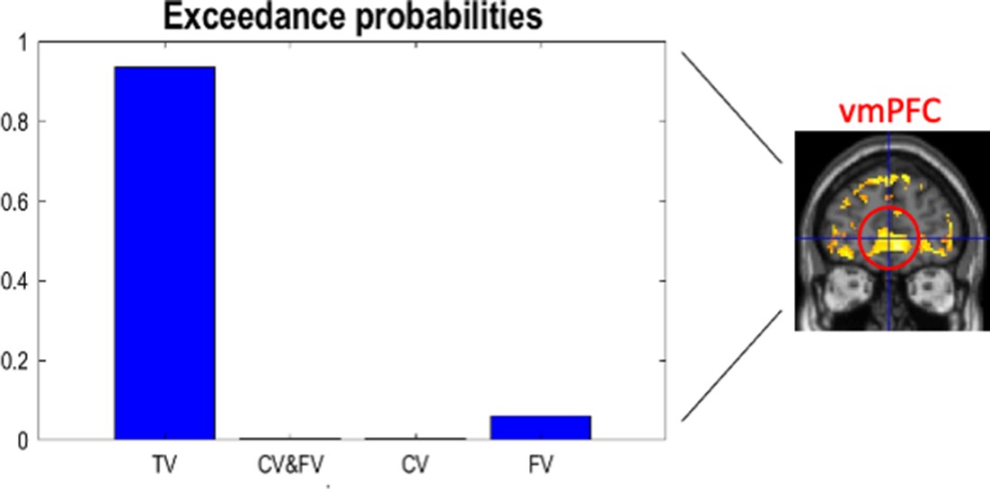
To confirm that the vmPFC is encoding total values rather than only current or future values, we performed cross-validate Bayesian model selection (cvBMS) at the neural level using the MACS toolbox in SPM (Soch and Allefeld, 2018). We compared four different GLMs: (i) the GLM with total value (TV; our original GLM), (ii) the GLM with both current and future value without orthogonalization (CV & FV), (iii) the GLM with only current value (CV), and (iv) the GLM with only future value (FV), all estimates from the 2-step forward thinking (FT) model. First, we assessed each model at the individual level using the cross-validated log model evidence (cvLME) and computed exceedance probability (EP) of each model at the group level. EP was highest for our original model in the vmPFC. Bar graphs represent EP of each model at [0, 48, 0]. The highlighted voxels in the whole-brain image represent where TV was selected as the optimal model.
Figure 5—figure supplement 4
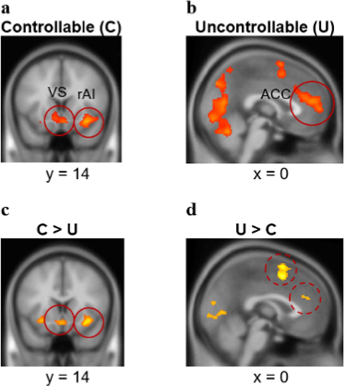
Norm prediction error signals.
Norm prediction error signals were found from (a) the ventral striatum (VS; [4, 14, −14]) and the right anterior insula (rAI; [32, 16, −14]) for the Controllable condition, while the signal was found from (b) the anterior cingulate cortex ([2, 46, 16]) for the Uncontrollable condition at PFWE<0.05, small volume corrected. These regions have been suggested to encode prediction errors in the similar norm learning context (Xiang et al., 2013). A whole-brain contrast of the two conditions revealed that (c) the VS ([4, 14, −14]) and the rAI ([32, 16, −14]) showed significantly greater BOLD responses for the Controllable than the Uncontrollable condition (PFWE<0.05, small volume corrected). However, (d) the ACC ([2, 46, 16]) response under the Uncontrollable condition was not significantly greater than the Controllable condition at the same threshold. Whole-brain analysis results were displayed at p<0.05, uncorrected, k>120. ACC, anterior cingulate cortex; BOLD, blood-oxygen-level-dependent.
Figure 5—figure supplement 5
Norm signals.
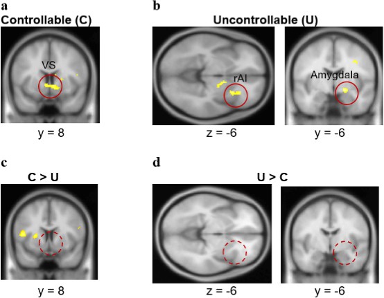
Norm-related BOLD signals were found (a) from the ventral striatum ([10, 16, −2]) for the Controllable condition, and (b) from the right anterior insula ([28, 16, −6]) and the amygdala ([18, −6, −8]) for the Uncontrollable condition at PFWE<0.05, small volume corrected. (c, d) However, whole-brain contrast showed no difference between the conditions. Displayed at p<0.01, uncorrected, k>50. BOLD, blood-oxygen-level-dependent.
Appendix 1—figure 1

Task design for online study’ and caption: Screen #6–11: Practice rounds.
Screen #14–15: Team assignment. Displayed at the beginning of each condition. Screen #16–20: One round of the actual task; repeated 30 times for each team (condition). The order of partners (avatars and names) were randomized. Duration: Screen #16 (avatar): 1.5–2.5 s; jittered, screen #17 (choice): self-paced, screen #18 (post-choice), #19 (outcome), #20 (fixation): 1 s.
Author response image 1
Tables
Table 1
Parameter estimates from the 2-step forward thinking (FT) model.
| Inverse temperature | Sensitivity to norm violation | Initial norm | Adaptation rate | Expected influence | |
|---|---|---|---|---|---|
| Mean (SD) | β | α | f0 | ε | δ |
| Controllable | |||||
| fMRI sample | 8.33 (8.55) | 0.76 (0.29) | 8.21 (7.14) | 0.24 (0.24) | 1.33 (0.79) |
| Online sample | 9.77 (8.54) | 0.74 (0.29) | 9.01 (7.26) | 0.32 (0.31) | 1.34 (0.84) |
| Uncontrollable | |||||
| fMRI sample | 10.38 (8.84) | 0.79 (0.31) | 8.84 (6.96) | 0.29 (0.24) | 0.98 (0.62) |
| Online sample | 12.94 (7.66) | 0.78 (0.23) | 9.07 (6.31) | 0.24 (0.24) | 0.90 (1.06) |
Author response table 1
| Estimate | SE | t | p | |
|---|---|---|---|---|
| Intercept | 2.87 | 0.61 | 4.70 | 0.00 |
| vmPFC | -0.26 | 0.16 | -1.60 | 0.12 |
| PC | 0.01 | 0.01 | 1.51 | 0.14 |
| Δ | 1.76 | 0.21 | 8.34 | 0.00 |
Author response table 3
| Name | Estimate | SE | t | DF | p-value |
|---|---|---|---|---|---|
| Intercept | 1.60 | 0.06 | 28.72 | 2860 | 0.000 |
| Condition (***) | 0.13 | 0.03 | 4.39 | 2860 | 0.000 |
| Conflict (**) | -0.04 | 0.01 | -2.98 | 2860 | 0.003 |
| Condition × conflict | 0.03 | 0.02 | 1.66 | 2860 | 0.096 |
Author response table 2
| Name | Estimate | SE | t | DF | p-value |
|---|---|---|---|---|---|
| Intercept | 1.52 | 0.06 | 24.43 | 2860 | 0.000 |
| Condition (***) | 0.21 | 0.06 | 3.71 | 2860 | 0.000 |
| Chosen value | 0.00 | 0.01 | 0.48 | 2860 | 0.630 |
| Condition × chosen value | 0.00 | 0.01 | -0.80 | 2860 | 0.426 |
Additional files
-
Supplementary file 1
Supplementary tables.
- https://cdn.elifesciences.org/articles/64983/elife-64983-supp1-v1.docx
-
Supplementary file 2
Task instructions.
- https://cdn.elifesciences.org/articles/64983/elife-64983-supp2-v1.docx
-
Transparent reporting form
- https://cdn.elifesciences.org/articles/64983/elife-64983-transrepform1-v1.pdf
Download links
A two-part list of links to download the article, or parts of the article, in various formats.
Downloads (link to download the article as PDF)
Open citations (links to open the citations from this article in various online reference manager services)
Cite this article (links to download the citations from this article in formats compatible with various reference manager tools)
Humans use forward thinking to exploit social controllability
eLife 10:e64983.
https://doi.org/10.7554/eLife.64983


