GluA4 facilitates cerebellar expansion coding and enables associative memory formation
- Department of Molecular Life Sciences, University of Zurich, Switzerland
- Neuroscience Center Zurich, Switzerland
- Champalimaud Neuroscience Programme, Champalimaud Centre for the Unknown, Portugal
Figures
Figure 1 with 3 supplements
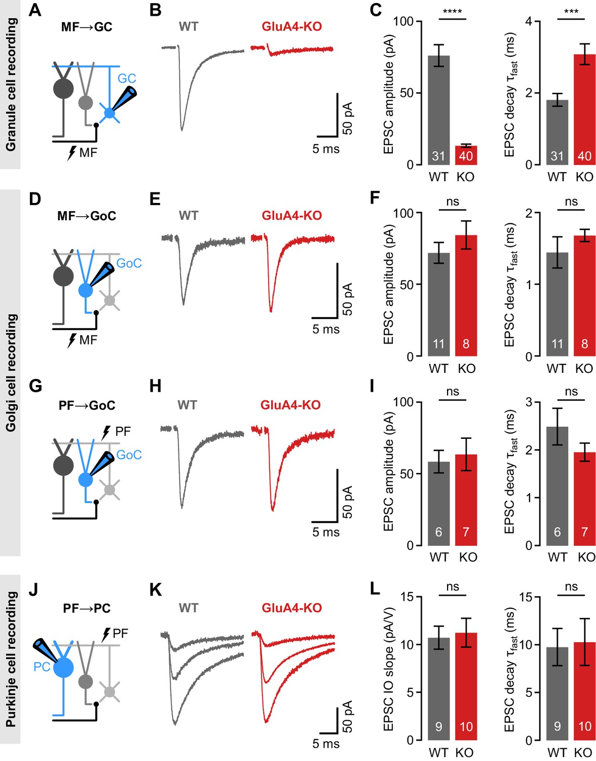
Selective impairment of cerebellar mossy fiber (MF)→granule cell (GC) synapses in GluA4-knockout (GluA4-KO) mice.
(A) Schematic of recordings from MF→GC connections. (B) Example excitatory postsynaptic currents (EPSCs) recorded from wild-type (WT) and KO GCs by single MF stimulation. (C) Average EPSC amplitude (left; p < 0.0001; Cohen’s d = −2.23) and average EPSC fast decay time constant (right; p < 0.001; d = 0.84) for WT and KO MF→GC EPSCs. Data are redrawn from Delvendahl et al., 2019. (D) Recordings from MF→Golgi cell (GoC) connections. (E) Example EPSCs upon MF stimulation recorded from GoCs. (F) Average EPSC amplitude (left; p = 0.32; d = 0.49) and fast decay time constant (right; p = 0.33; d = 0.42) for WT and KO MF→GoC EPSCs. (G) Recordings from parallel fiber (PF)→GoC connections. (H) Example EPSCs recorded from GoCs upon PF stimulation. (I) Average EPSC amplitude (left; p = 0.73; d = 0.19) and fast decay time constant (right; p = 0.25; d = −0.73) for WT and KO PF→GoC EPSCs. (J) Recordings from PF→Purkinje cell (PC) connections. (K) Example EPSCs recorded from PCs by stimulating afferent PFs with increasing stimulation strength (displayed stimulation intensities: 7, 12, and 17 V). (L) Average linear slope of the stimulus-response relationship (left; p = 0.79; d = 0.12) and fast decay time constant (right; p = 0.87; d = 0.08) for WT and KO PF→PC EPSCs. Data are means ± SEM.
-
Figure 1—source data 1
Numerical data plotted in Figure 1.
- https://cdn.elifesciences.org/articles/65152/elife-65152-fig1-data1-v2.xlsx
Figure 1—figure supplement 1
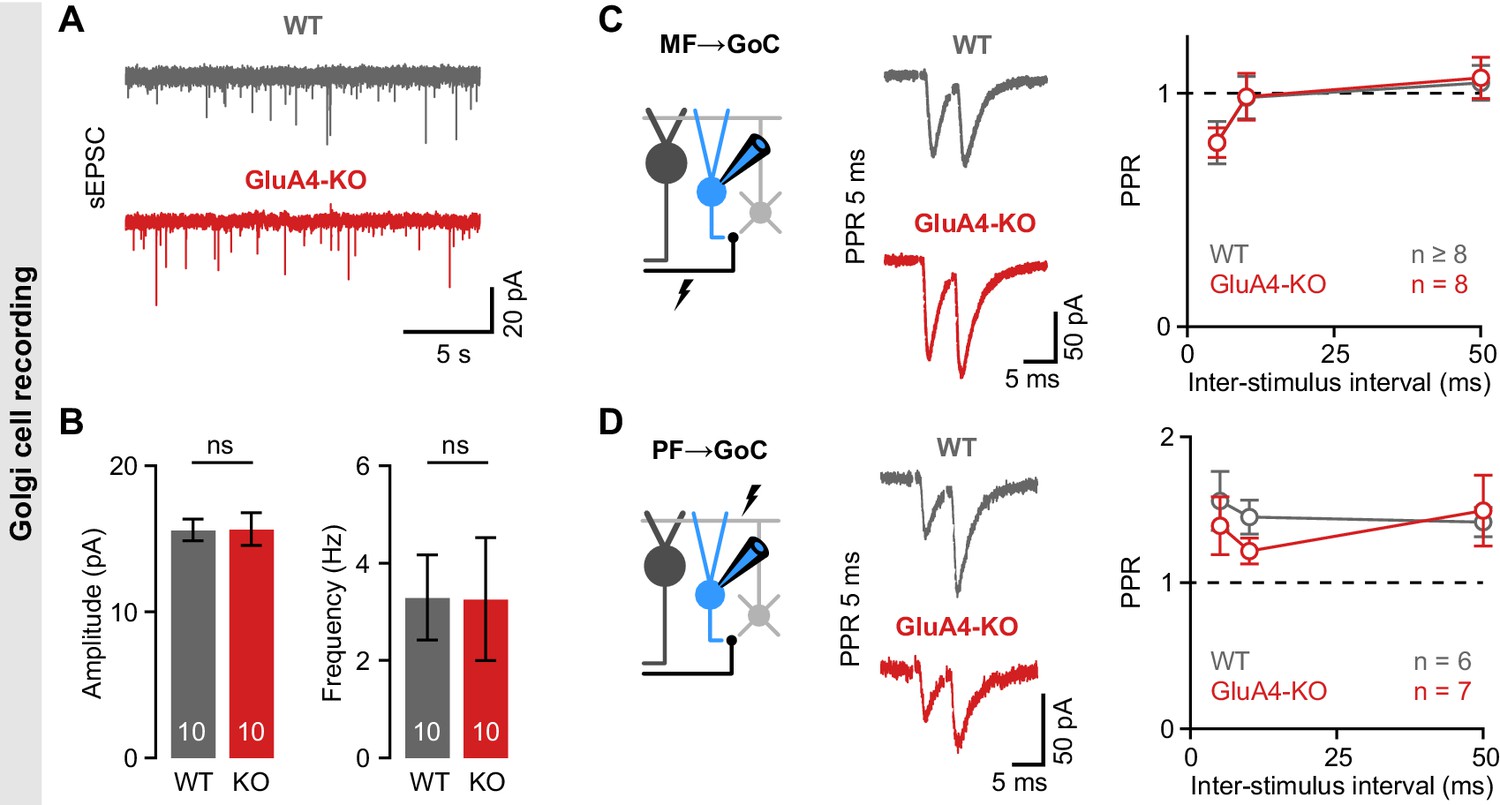
Unaltered transmission at excitatory synapses in cerebellar Golgi cells (GoCs).
(A) Example spontaneous excitatory postsynaptic current (sEPSC) recordings from wild-type (WT) and GluA4-knockout (GluA4-KO) GoCs. (B) Average sEPSC amplitudes (left; p = 0.96) and frequency (right; p = 0.98) for both genotypes. (C) Left: Schematic of recordings from mossy fiber (MF)→GoC connections. Middle: Example paired-pulses at 5 ms inter-stimulus interval for WT and GluA4-KO. Right: Average paired-pulse ratios (PPR) vs. inter-stimulus interval for both genotypes. (D) Same as (C), but for parallel fiber (PF)→GoC connections. Data are means ± SEM.
Figure 1—figure supplement 2
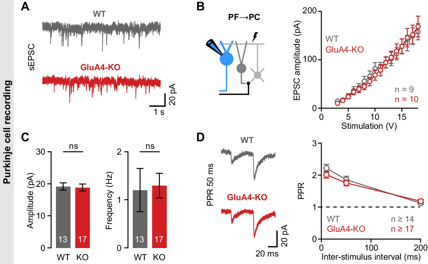
Unaltered transmission at excitatory synapses in cerebellar Purkinje cells (PCs).
(A) Example spontaneous excitatory postsynaptic current (sEPSC) recordings from wild-type (WT) and GluA4-knockout (GluA4-KO) PCs. (B) Average sEPSC amplitude (left; p = 0.84) and frequency (right; p = 0.0.85) for both genotypes. (C) Left: Schematic of EPSC recordings from parallel fiber (PF)→PC connections. Right: PF→PC EPSC amplitude as a function of stimulation intensity. (D) Left: Example paired-pulses at 50 ms inter-stimulus interval. Right: Average paired-pulse ratio (PPR) vs. inter-stimulus interval for WT and GluA4-KO PCs. Data are means ± SEM.
Figure 1—figure supplement 3
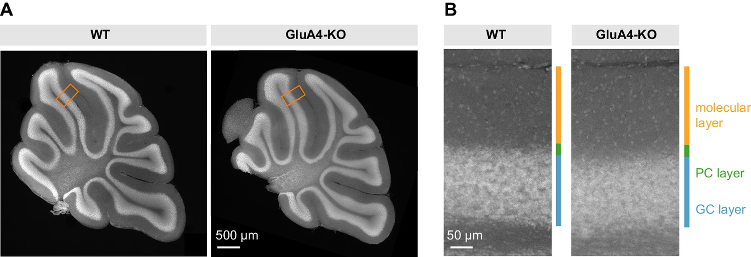
Unaltered gross cerebellar organization.
(A) DAPI stained sagittal cerebellar sections of wild-type (WT) and GluA4-knockout (GluA4-KO) mice. (B) Higher magnifications of (A) as indicated by orange boxes. Relative thickness of granule cell (GC) layer, Purkinje cell (PC) layer, and molecular layer was not changed in GluA4-KO mice. Similar results were obtained in n = 5 experiments.
Figure 2 with 3 supplements
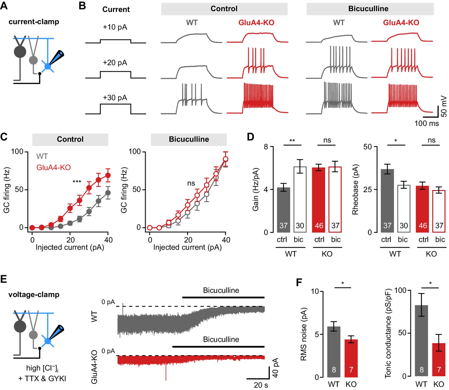
Reduced tonic inhibition increases the granule cell (GC) input-output relationship.
(A) Current-clamp recordings from GCs. (B) Example responses to somatic current injection of indicated amplitude for control and in the presence of 10 µM bicuculline. (C) Average GC firing frequency plotted vs. injected current for wild type (WT) and knockout (KO) in control and bicuculline. (D) Average gain and rheobase, calculated from the frequency-current curves in (C). In the presence of bicuculline, KO GCs had gain and rheobase values comparable to WT. (E) Recording of tonic holding current. GABAergic currents were isolated using 20 µM GYKI-53655 and an intracellular solution with high [Cl−] to maximize GABAA receptor-mediated currents (see Materials and methods). Right: Example recordings of bicuculline wash-in (10 µM) for WT and KO GCs. (F) Average root-mean-square noise before wash-in of bicuculline (left; p = 0.048; d = −1.11) and average tonic conductance density (right; p = 0.020; d = −1.35) for WT and GluA4-KO. Tonic conductance was calculated from the bicuculline-sensitive current. Data are means ± SEM.
-
Figure 2—source data 1
Numerical data plotted in Figure 2.
- https://cdn.elifesciences.org/articles/65152/elife-65152-fig2-data1-v2.xlsx
Figure 2—figure supplement 1
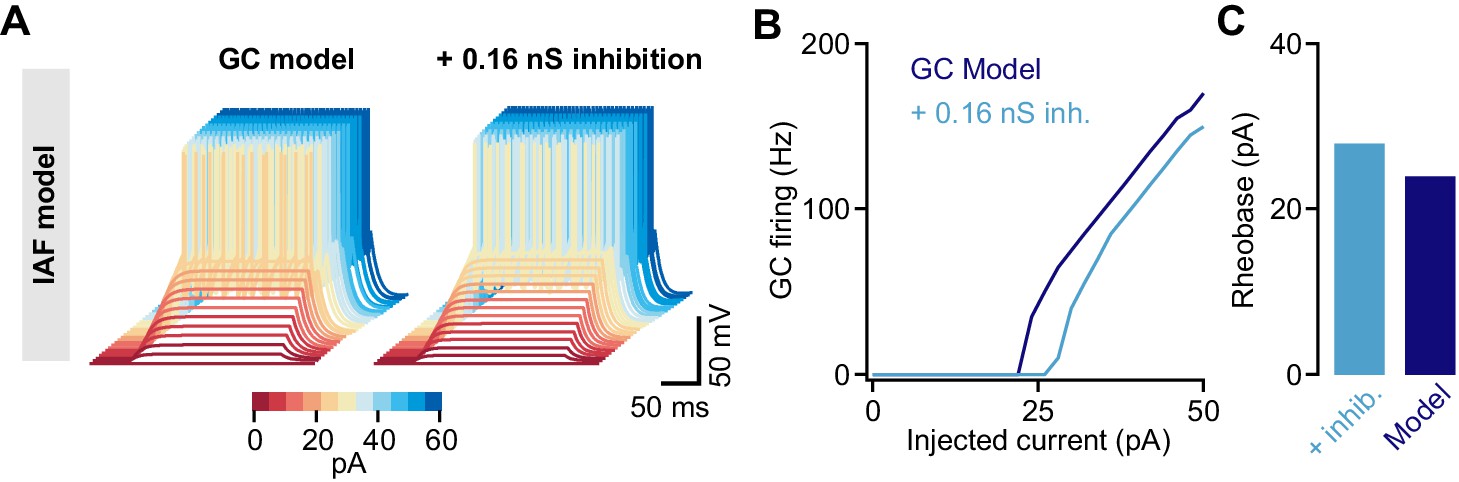
Tonic inhibition in a cerebellar granule cell (GC) integrate-and-fire model.
(A) Membrane voltages of an integrate-and-fire (IAF) model in response to current injections of increasing amplitude (color coded). Adding 0.16 nS tonic inhibitory conductance reduces excitability. (B) Action potential firing frequency vs. injected current for the model with (light blue) and without (dark blue) tonic inhibition. (C) Rheobase current of the IAF model for both conditions.
Figure 2—figure supplement 2
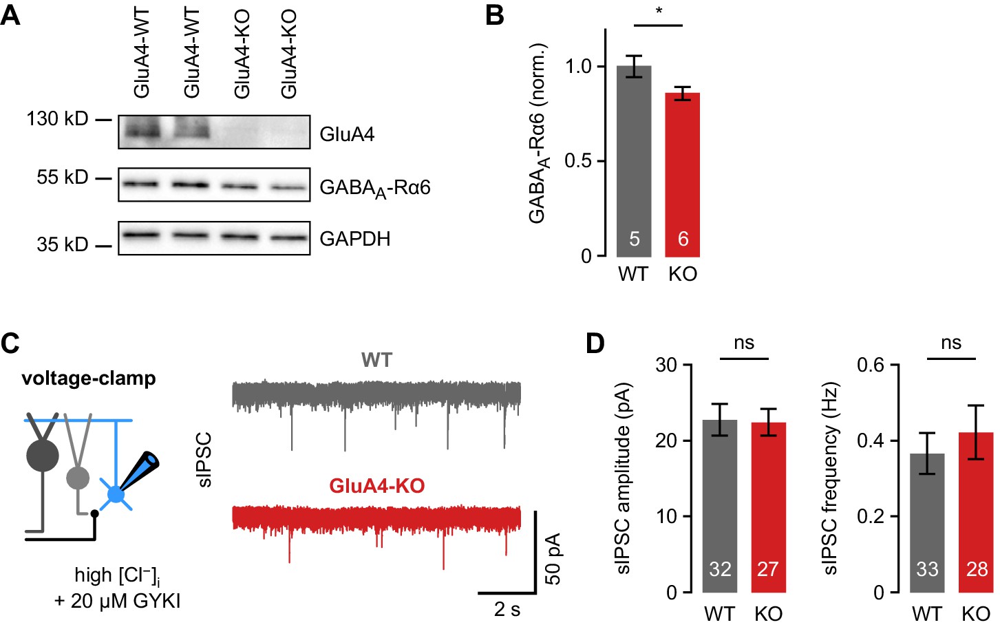
Phasic inhibition in cerebellar granule cells (GCs) of wild-type (WT) and GluA4-knockout (GluA4-KO) mice.
(A) Western blot of cerebellar lysates from mice of indicated genotypes labeled for GluA4, α6 GABAA receptor (GABAAR) subunit (GABAA-Rα6), and GAPDH. (B) Normalized α6 GABAAR expression in WT and GluA4-KO (p = 0.028). Data are normalized to GAPDH and WT, and are averages of two to four technical and five to six biological replicates (per genotype). (C) Left: Spontaneous inhibitory postsynaptic current (sIPSC) recordings in GCs. Inhibitory currents were isolated using 20 µM GYKI-53655 and a CsCl-based intracellular solution. Right: Example sIPSC recordings from WT and GluA4-KO GCs. (D) Average sIPSC amplitude (left; p = 0.54) and frequency (right; p = 0.53) for WT and GluA4-KO. Data are means ± SEM.
Figure 2—figure supplement 3
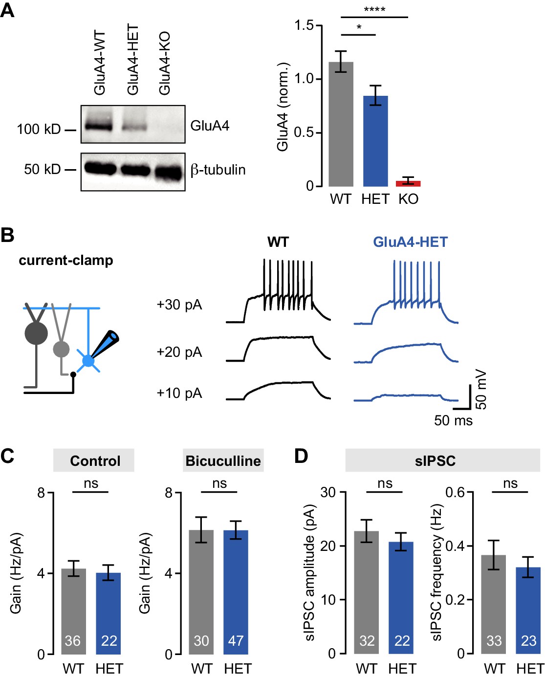
Normal tonic and phasic inhibition in heterozygous GluA4 (GluA4-HET) granule cells (GCs).
(A) Left: Western blot of cerebellar lysates from indicated genotypes labeled for GluA4 and β-tubulin. Right: Normalized GluA4 expression in wild type (WT), GluA4-HET, and GluA4-knockout (GluA4-KO). Data are normalized to β-tubulin and are averages of three technical and five biological replicates (per genotype). (B) Example responses to somatic current injection of indicated amplitude for WT and GluA4-HET under control conditions. (C) Average gain of the frequency-current relationship for control (left; p = 0.77) and bicuculline (right; p = 0.22). (D) Average spontaneous inhibitory postsynaptic current (sIPSC) amplitude (left; p = 0.28) and frequency (right; p = 0.53) for WT and GluA4-HET. Data are means ± SEM.
Figure 3 with 2 supplements
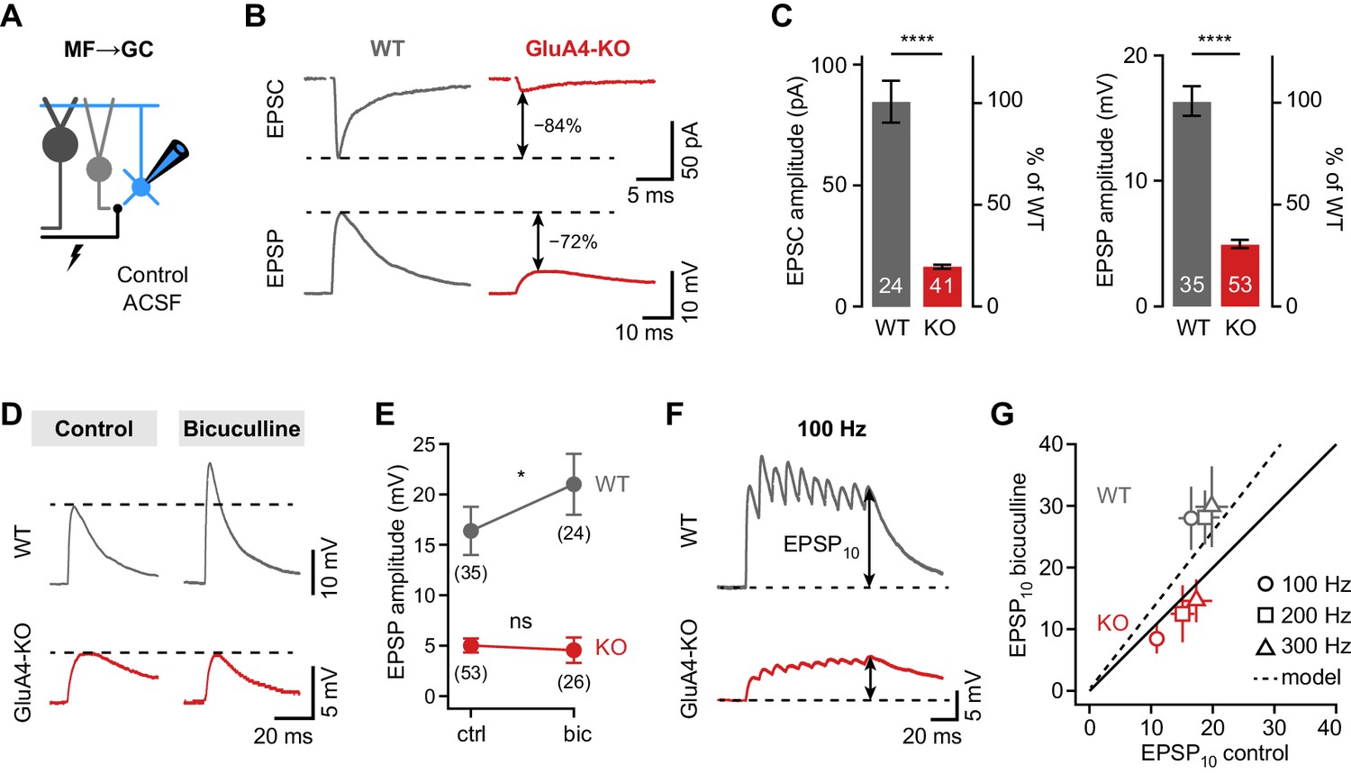
Shunting inhibition controls excitatory postsynaptic potential (EPSP) size in cerebellar granule cells (GCs).
(A) Recordings from mossy fiber (MF)→GC connections in voltage- or current-clamp with blocker-free artificial cerebrospinal fluid (ACSF) (‘control’). (B) Example excitatory postsynaptic current (EPSC) and excitatory postsynaptic potential (EPSP) recordings from the same cell in wild type (WT) and knockout (KO). Arrows indicate reduction compared to WT. (C) Average EPSC (left, p < 0.0001, d = −2.62) and EPSP amplitudes (right, p < 0.0001, d = −2.37) for WT and KO. Note the difference in relative reduction of EPSPs compared to EPSCs. (D) Example EPSP recordings for control and in the presence of 10 µM bicuculline. (E) Average EPSP amplitude for WT and KO. Error bars represent 95% CI. (F) Example MF→GC EPSP trains (10 stimuli, 100 Hz). (G) Average EPSP10 in the presence of bicuculline vs. control for the indicated stimulation frequencies. Black line represents unity and dashed line the prediction of an integrate-and-fire model with or without tonic inhibition (Figure 2—figure supplement 1). Data in (C) and (G) are means ± SEM.
-
Figure 3—source data 1
Numerical data plotted in Figure 3.
- https://cdn.elifesciences.org/articles/65152/elife-65152-fig3-data1-v2.xlsx
Figure 3—figure supplement 1
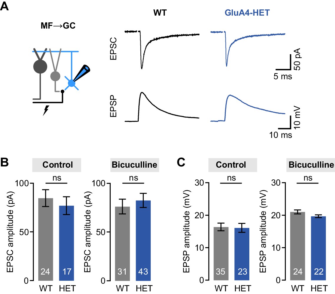
Normal mossy fiber (MF)→granule cell (GC) excitatory postsynaptic currents (EPSCs) and excitatory postsynaptic potentials (EPSPs) in heterozygous GluA4 (GluA4-HET) GCs.
(A) Example EPSCs and EPSPs for wild type (WT) and GluA4-HET under control conditions. (B) Average EPSC amplitude for WT and GluA4-HET for control and bicuculline. Bicuculline data are redrawn from Delvendahl et al., 2019. (C) Average EPSP amplitude for WT and GluA4-HET. Note that EPSPs were larger in both genotypes in the presence of bicuculline. Data are means ± SEM. n.s. p > 0.05.
Figure 3—figure supplement 2
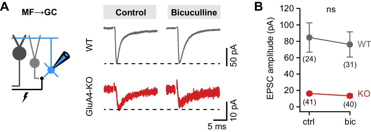
Similar mossy fiber (MF)→granule cell (GC) excitatory postsynaptic current (EPSC) amplitudes between control and bicuculline.
(A) Example MF→GC EPSCs in wild-type (WT) and GluA4-knockout (GluA4-KO) GCs for control and bicuculline. (B) Average EPSC amplitude of WT and GluA4-KO was not different between control (‘ctrl’) and bicuculline (‘bic’) (ANOVA drug × genotype: F = 0.35, p = 0.56, η2p = 0.003). Data are means ± 95% confidence interval.
Figure 4 with 3 supplements
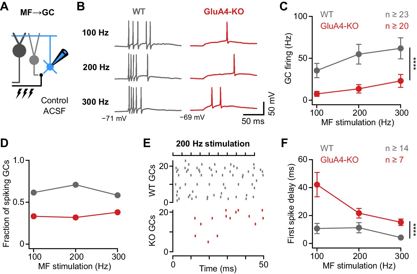
Deletion of GluA4 impairs granule cell (GC) spike fidelity and precision during high-frequency transmission.
(A) Recordings from mossy fiber (MF)→GC connections in current-clamp. GCs were held at −70 mV. (B) Example voltage recordings from a wild type (WT) and GluA4-knockout (GluA4-KO) GC upon MF stimulation with 10 stimuli at increasing frequencies (indicated). (C) Average GC firing frequency upon MF stimulation with 100–300 Hz frequency. (D) Fraction of GCs showing spikes upon 100–300 Hz MF stimulation. (E) Spike raster plots for 200 Hz MF stimulation in WT and GluA4-KO. (F) Average first spike delay calculated from stimulation onset plotted vs. MF stimulation frequency. Data are means ± SEM.
-
Figure 4—source data 1
Numerical data plotted in Figure 4.
- https://cdn.elifesciences.org/articles/65152/elife-65152-fig4-data1-v2.xlsx
Figure 4—figure supplement 1
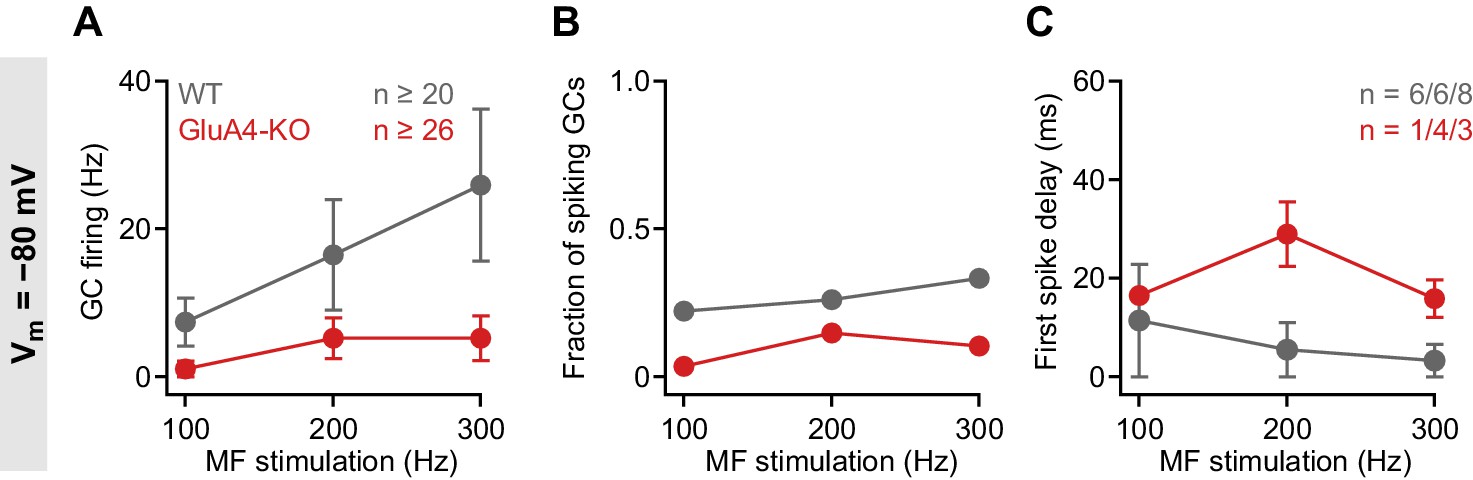
Impaired granule cell (GC) spike output in GluA4-knockout (GluA4-KO) GCs at −80 mV.
(A) Average GC firing frequency upon mossy fiber (MF) stimulation with 100–300 Hz frequency for wild type (WT) and GluA4-KO. GC membrane voltage was maintained at −80 mV by current injection. (B) Fraction of GCs showing spikes upon MF stimulation with 100–300 Hz frequency. (C) Average first spike delay plotted vs. MF stimulation frequency; delay was calculated from stimulation onset. Data are means ± SEM.
Figure 4—figure supplement 2
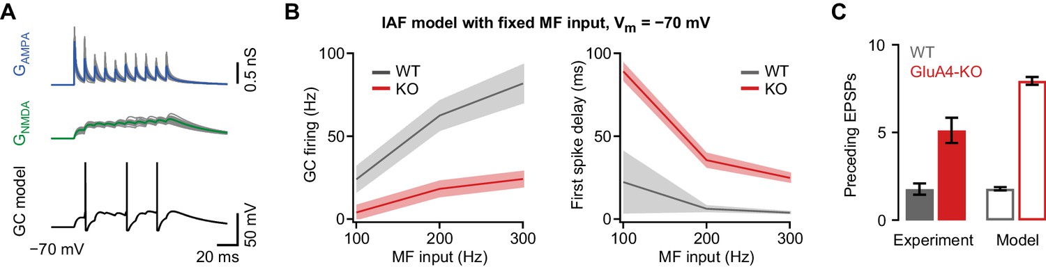
Impaired granule cell (GC) spiking in an integrate-and-fire (IAF) GC model.
(A) Top: Simulated 100 Hz AMPA receptor (AMPAR) (GAMPA, blue) and NMDA receptor (NMDAR) conductances (GNMDA, green) using a binomial model of short-term plasticity (20 individual traces in gray overlaid with averages in color). Bottom: Result of single simulation using a GC IAF model (black; Figure 2—figure supplement 1) with wild-type (WT) GAMPA and GNMDA. (B) Left: Average model firing frequency upon mossy fiber (MF) input with 100–300 Hz frequency. The model included either WT or GluA4-knockout (GluA4-KO) synaptic conductances as indicated. Right: Average first spike delay calculated from stimulation onset plotted vs. MF stimulation frequency. Data are means, shadows represent SD. (C) Average number of excitatory postsynaptic potentials (EPSPs) preceding the first GC spike for WT and GluA4-KO (300 Hz MF stimulation) together with corresponding results from simulation. Data are means ± SEM.
Figure 4—figure supplement 3
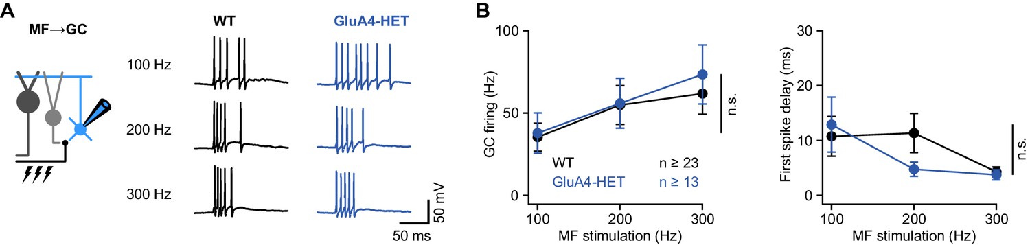
Normal granule cell (GC) spike output in heterozygous GluA4 (GluA4-HET) GCs.
(A) Example voltage recordings from a wild-type (WT) and GluA4-HET GC upon mossy fiber (MF) stimulation with 10 stimuli at increasing frequencies (indicated). GC membrane voltage was maintained at −70mV. (B) Left: Average GC firing frequency upon MF stimulation with 100–300 Hz frequency (ANOVA genotype: F = 0.22, p = 0.64, η2p = 0.002). Right: Average first spike delay (calculated from stimulation onset) plotted vs. MF stimulation frequency. Data are means ± SEM. n.s. p > 0.05.
Figure 5 with 2 supplements
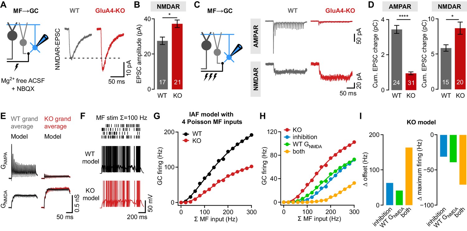
NMDA receptors (NMDARs) and reduced inhibition support spiking in GluA4-knockout (GluA4-KO) granule cells (GCs).
(A) Left: Recordings of isolated NMDAR-EPSCs (excitatory postsynaptic currents) at mossy fiber (MF)→GC connections. Right: Example NMDAR-mediated MF→GC EPSCs. (B) Average EPSC amplitude for wild-type (WT) and GluA4-KO GCs (p = 0.0026; d = 1.04). (C) Left: Schematic of MF→GC train stimulation. Top: Example AMPA receptor (AMPAR)-EPSC 100 Hz train recordings (20 stimuli) for WT and KO. Bottom: Example NMDAR-mediated 100 Hz trains. (D) Average cumulative charge for AMPAR-mediated (left; p < 0.0001; d = −3.05) and NMDAR-mediated EPSCs (right; p = 0.0063; d = 0.92) for both genotypes. (E) Grand average of AMPAR and NMDAR conductance trains (20 stimuli, 100 Hz) recorded from WT (left) and GluA4-KO GCs (right). Data are overlaid with synaptic conductance models for WT and GluA4-KO. (F) Top: Four independent Poisson-distributed MF spike trains with a sum of 100 Hz (top) and simulation results for WT (black) and KO (red). (G) Average WT and KO model firing frequency vs. MF stimulation frequency. Lines are fits with a Hill equation. (H) Results for KO model compared with simulations of KO GCs with tonic inhibition (blue), with WT GNMDA (green) or both (yellow). (I) Reduced inhibition and enhanced GNMDA reduce the offset (left) and increase the maximum firing frequency (right) of the KO model GC output. Data are means ± SEM.
-
Figure 5—source data 1
Numerical data plotted in Figure 5.
- https://cdn.elifesciences.org/articles/65152/elife-65152-fig5-data1-v2.xlsx
Figure 5—figure supplement 1
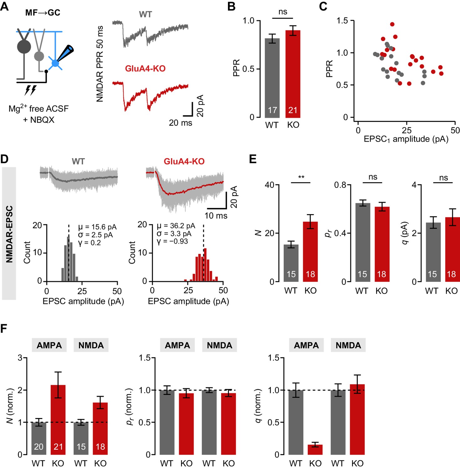
Increased number of presynaptic release sites in GluA4-knockout (GluA4-KO) mice.
(A) Example mossy fiber (MF)→granule cell (GC) paired-pulses at 50 ms inter-stimulus interval. NMDA receptor (NMDAR)-mediated excitatory postsynaptic currents (EPSCs) were isolated using 10 µM NBQX and 0 mM external Mg2+. (B) Average paired-pulse ratio (PPR) for wild-type (WT) and GluA4-KO GCs (p = 0.23). (C) NMDAR-PPR vs. amplitude of the first EPSC (EPSC1). (D) Top: Example NMDAR-EPSC recordings. Shown are 60 individual sweeps overlaid with the average. Bottom: Histogram of EPSC amplitudes for the examples shown above. Mean (μ), standard deviation (σ), and skewness (γ) are indicated. (E) Quantification of the number of release sites (N; p = 0.0064, d = 0.98), release probability (pr; p = 0.50, d = −0.23), and quantal size (q; p = 0.60, d = 0.18) for WT and GluA4-KO. Statistical moments analysis of quanta (‘SMAQ’, Holler et al., 2021) was used to estimate binomial parameters from NMDAR-EPSCs. (F) Normalized SMAQ-derived N, pr, and q for AMPAR- and NMDAR-mediated EPSCs (normalized to WT). Data are means ± SEM.
Figure 5—figure supplement 2
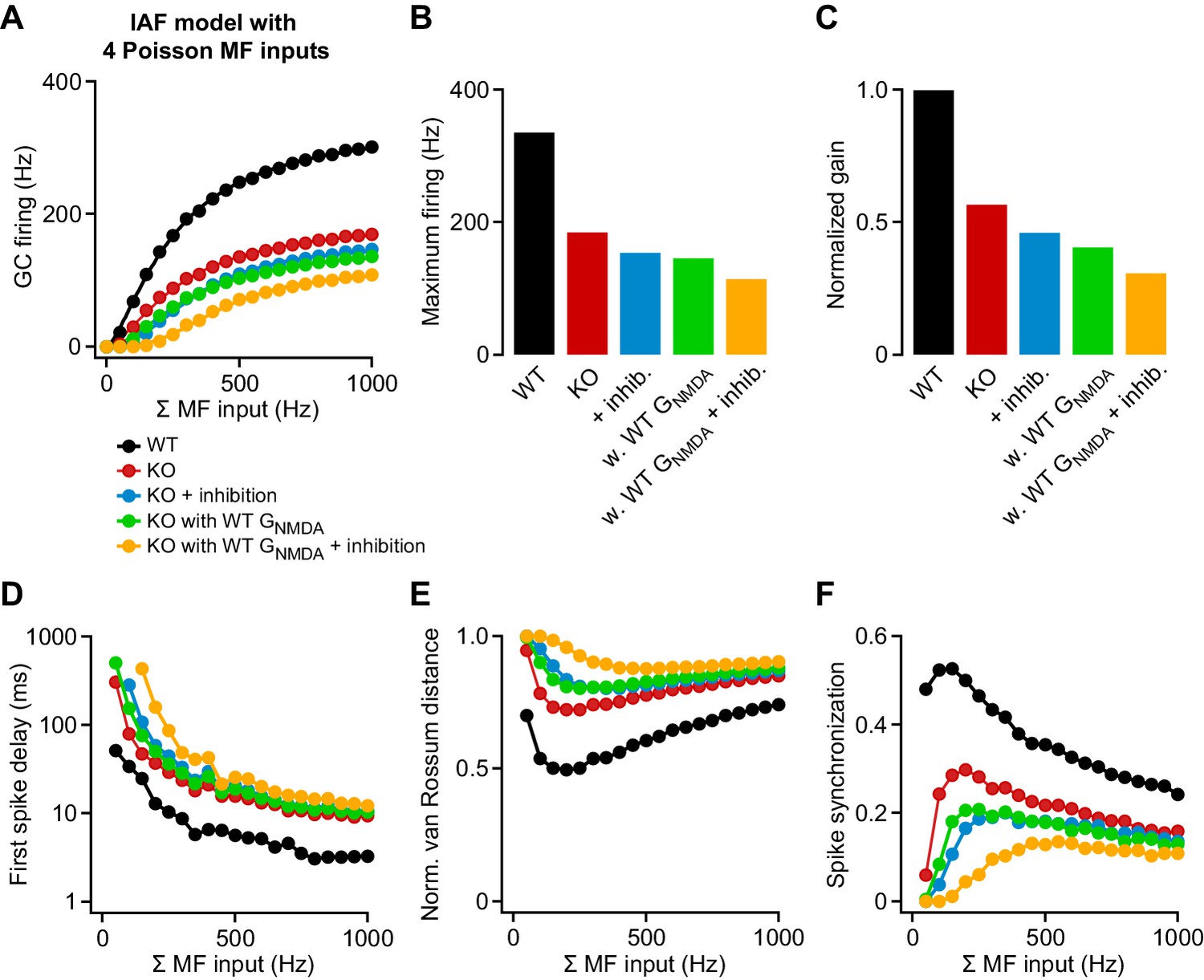
Contribution of attenuated inhibition and enhanced GNMDA to granule cell (GC) spike output.
(A) Average wild-type (WT) and knockout (KO) model firing frequency vs. mossy fiber (MF) input frequency for a range of 50–1000 Hz. Lines are fits with a Hill equation (see Materials and methods). (B) Maximum firing frequency determined from fits to the data in (A). (C) Gain of the input-output relation, normalized to the WT simulation. (D) Average first spike delay vs. MF input frequency. Note the log scale of the ordinate. (E) Normalized van Rossum distance vs. MF input frequency. The van Rossum distance was calculated using an exponential kernel with τ = 10 ms, and normalized to the maximum error for each frequency (calculated for all random MF spike trains without postsynaptic spikes). (F) Spike synchronization (see Materials and methods) vs. MF input frequency of 50–1000 Hz. Larger values indicate higher synchrony of pre- and postsynaptic spikes.
Figure 6 with 1 supplement

Impaired pattern separation in a feedforward model of the cerebellar input layer.
(A) Schematic of the feedforward network model. The model comprises 187 mossy fibers (MFs) that are connected to 487 granule cells (GCs) with four synapses per GC. The network is presented with different MF activity patterns, which produce GC spike patterns. (B) Histogram of active GCs. Scaling synaptic (AMPA receptor [AMPAR] and NMDA receptor [NMDAR]) conductance and tonic inhibitory conductance according to the GluA4-knockout (GluA4-KO) data (‘KO model’, red) leads to strong reduction of active GCs compared to the model from Cayco-Gajic et al., 2017 (‘control’, black). (C) Left: Normalized population sparseness (normalized to MF sparseness) plotted for different MF correlation radii and fraction of active MFs of both models. Right: Median normalized sparseness vs. MF correlation radius. Median is calculated across fractions of active MFs. (D) Same as (C), but for total variance. (E) Schematic of learning implementation. MF or GC activity patterns are used to train a perceptron decoder to classify these patterns into 10 random classes. (F) Root-mean-square (RMS) error of the perceptron classification for MF input patterns (blue), GC input patterns (black) or GC patterns with scaled conductance (red). Dashed line indicates cutoff for learning speed quantification. (G) Left: Normalized learning speed (normalized to learning using MF patterns) plotted for different MF correlation radii and fraction of active MFs of both models. White dashed borders indicate areas of faster learning with GC activity patterns than with MF patterns. Right: Median normalized learning speed vs. MF correlation radius. Dashed line indicates faster GC learning.
Figure 6—figure supplement 1
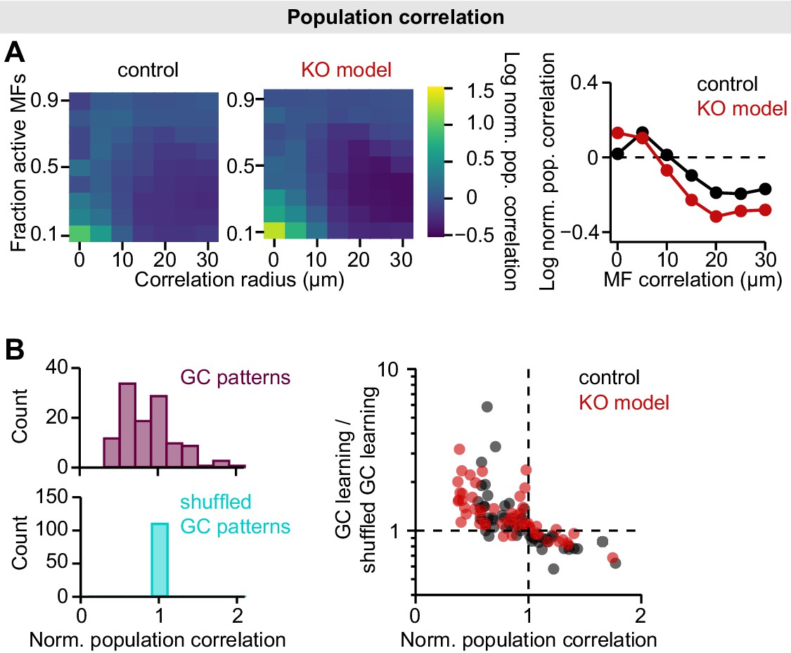
Population correlations in the mossy fiber (MF)-granule cell (GC) feedforward model.
(A) Left: Log-normalized population correlation (see Materials and methods; normalized to MF correlations) plotted for different MF correlation radii and fraction of active MFs of both models. Right: Median log-normalized population correlation vs. MF correlation radius. Data points below dashed line indicate active decorrelation. Median is calculated across fractions of active MFs. (B) To assess the contribution of decorrelation to learning speed, we used shuffled GC patterns to train the perceptron (Cayco-Gajic et al., 2017). GC patterns were shuffled to achieve the same population correlation as MF patterns, while preserving sparseness and total variance. Left: Histograms of normalized GC population correlation before and after shuffling. Right: The contribution of decorrelation to learning speed is similar in both models. GC learning speed is normalized to speed using shuffled patterns and plotted vs. population correlation.
Figure 7 with 3 supplements

Normal locomotor coordination of GluA4-knockout (GluA4-KO) mice during overground walking.
(A) LocoMouse apparatus. (B) Continuous tracks (in x, y, z) for nose, paws, and tail segments obtained from LocoMouse tracking (Machado et al., 2015) are plotted on top of the frame. (C) Individual strides were divided into swing and stance phases for further analysis. (D)–(E) Stride length of front right (FR) paw (D) and hind right (HR) paw (E) vs. walking speed for GluA4-KO mice (red) and wild-type (WT) animals (gray). For each parameter, the thin lines with shadows represent median values ± 25th, 75th percentiles. (F)–(G) Average instantaneous forward (x) velocity of FR paw (F) and HR paw (G) during swing phase. (H)–(I) Average vertical (z) position of FR paw (H) and HR paw (I) relative to ground during swing. The shaded area indicates SEM across mice. (J)–(K) Polar plots indicating the phase of the step cycle in which each limb enters stance, aligned to stance onset of FR paw (red circle). Distance from the origin represents walking speed. (J) WT mice; (K) GluA4-KO mice. Circles show average values for each animal.
Figure 7—figure supplement 1
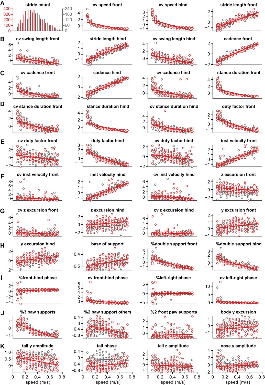
Distribution of z-scored values for all gait parameters.
Each circle represents the mean z-scored value of that gait parameter for one animal at one speed bin. Wild-type ( WT) animals are in gray and GluA4-knockout (GluA4-KO) animals in red. Lines are linear fits of each parameter for each animal group, across speed bins. Raw data for individual limb parameters (rows (A) to (H)). Interlimb parameters across speed bins (rows (H) to (J)). Whole body gait parameters over speed (last panel (J) and row (K)). Definitions of each parameter and method for calculating it are given in the Materials and methods section.
Figure 7—figure supplement 2
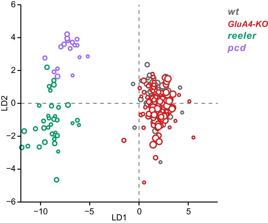
Linear discriminant analysis separates ataxic mutants from GluA4-knockout (GluA4-KO) and control animals.
Linear discriminant analysis of locomotor kinematics reveals two axes, which separate ataxic mutants from GluA4-KO and control (WT) animals (LD1) and from each other (LD2). The gait measurements from Figure 7—figure supplement 1 comprised the inputs to the LDA (see Materials and methods). Each circle represents a single animal walking at a particular speed. Faster speeds are shown with larger marker sizes. Speeds ranged from 0.05 to 0.8 m/s and were binned with a binwidth of 0.05 m/s. Size-matched controls for GluA4-KO animals are in gray (N = 9 for all speed bins), GluA4-KO animals are in red (N = 12 for all speed bins), reeler in green (N = 7 for 0.05–0.15 m/s; N = 6 for 0.25–0.35 m/s; n = ~2387), and pcd in purple (N = 3 for all speed bins except 0.25–0.30 m/s N = 2; n = ~3066). Reeler and pcd data are from Machado et al., 2015 and Machado et al., 2020a.
Figure 7—figure supplement 3

Normal locomotion in heterozygous GluA4 (GluA4-HET) mice.
(A)–(B) Stride length of front right (FR) paw (A) and hind right (HR) paw (B) vs. walking speed for GluA4-HET mice (blue) and wild-type (WT) animals (gray). For each parameter, the thin lines with shadows represent median values ± 25th, 75th percentiles. (C)–(D) Average instantaneous forward (x) velocity of FR paw (C) and HR paw (D) during swing phase. (E)–(F) Average vertical (z) position of FR paw (E) and HR paw (F) relative to ground during swing. The shaded area indicates SEM across mice. (G)–(H) Polar plots indicating the phase of the step cycle in which each limb enters stance, aligned to stance onset of FR paw (red circle). Distance from the origin represents walking speed. (G) WT mice; (H) GluA4-HET mice. Circles show average values for each animal.
Figure 8 with 1 supplement
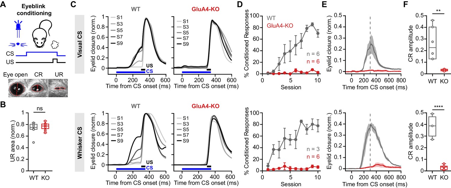
GluA4 is required for cerebellum-dependent associative memory formation.
(A) Top: Schematic of the eyeblink conditioning paradigm, where a conditioned stimulus (CS) (a white LED or a whisker vibratory stimulus) is repeatedly paired and co-terminates with an eyeblink-eliciting unconditioned stimulus (US) (a puff of air delivered to the eye). Bottom: Example video frames (acquired at 900 fps under infrared light) illustrate automated extraction of eyelid movement amplitude. (B) Normalized mean unconditioned response area for wild type (WT) and GluA4-knockout (GluA4-KO) (WT: n = 12; KO: n = 9; p = 0.36). (C) Average eyelid closure across nine learning sessions (S1–S9) of representative WT and KO animals, using a visual CS (top) or a whisker CS (bottom). Each trace represents the average of 100 paired trials from a single session. (D) Average %CR (% conditioned response) learning curves of WT (gray) and GluA4-KO (red) mice trained with either a visual CS (top) or a whisker CS (bottom). Error bars indicate SEM. (E) Average eyelid traces of CS-only trials from the last training session of WT and GluA4-KO animals, trained with either a visual CS (top) or a whisker CS (bottom). Shadows indicate SEM. Vertical dashed line represents the time that the US would have been expected on CS+US trials. (F) Average CR amplitudes from the last training session of WT and GluA4-KO animals, trained with either a visual CS (top; p = 0.0029) or a whisker CS (bottom; p < 0.0001). Box indicates median and 25th–75th percentiles; whiskers extend to the most extreme data points.
Figure 8—figure supplement 1
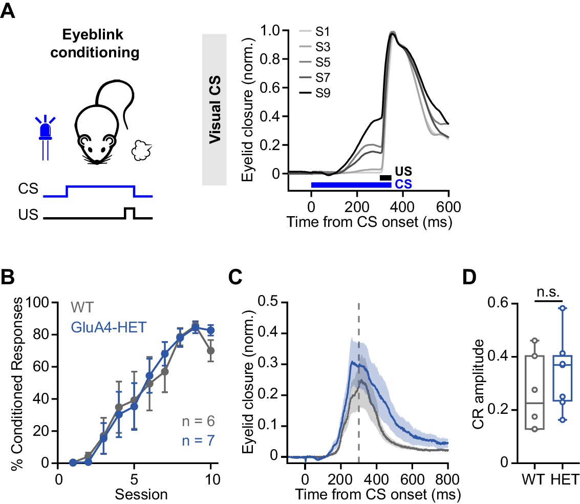
Normal associative learning in heterozygous GluA4 (GluA4-HET) mice.
(A) Left: Schematic of eyeblink conditioning experiment. Right: Average eyelid closure across nine learning sessions (S1–S9) of a representative wild-type (WT) animal using a visual conditioned stimulus (CS). Each trace represents the average of 100 paired trials from a single session. (B) Average %CR (% conditioned response) learning curves of WT (gray) and GluA4-HET (blue) mice. Error bars indicate SEM. (C) Average eyelid traces of CS-only trials from the last training session of WT and GluA4-HET animals. Shadows indicate SEM. Vertical dashed line represents the time that the unconditioned stimulus (US) would have been expected on CS+US trials. (D) Average CR amplitudes from the last training session of WT and GluA4-HET animals. Box indicates median and 25th–75th percentiles; whiskers extend to the most extreme data points. n.s. p > 0.05.
Videos
Video 1
Locomotion analysis of wild-type (WT) and GluA4-knockout (GluA4-KO) mice.
High-speed (400 fps) video of a mouse crossing the LocoMouse corridor, displayed at 30 fps. Side and bottom (via mirror reflection) views of the mouse are captured in a single camera. Top: Raw video of a WT mouse. Bottom: Raw video of a GluA4-knockout (GluA4-KO) mouse.
Tables
Key resources table
| Reagent type (species) or resource | Designation | Source or reference | Identifiers | Additional information |
|---|---|---|---|---|
| Strain, strain background (Mus musculus, ♀ and ♂) | Gria4tm1.1Mony/Gria4tm1.1Mony(‘GluA4-KO’) | Fuchs et al., 2007 | RRID:MGI:3804915 | |
| Antibody | Anti-GluA4 F-9 (mouse monoclonal) | Santa Cruz Biotechnology | Cat. # sc-271894 RRID:AB_10715096 | WB (1:100–1:200) |
| Antibody | Anti-GABAAR-α6 (rabbit polyclonal) | Alomone | Cat. # AGA-004 RRID:AB_2039868 | WB (1:500) |
| Antibody | Anti-GAPDH GA1R (mouse monoclonal) | Thermo Fisher Scientific | Cat. # MA5-15738-1MG RRID:AB_2537652 | WB (1:2000) |
| Antibody | Anti-β-tubulin (mouse monoclonal) | Developmental Studies Hybridoma Bank | Cat. # E7 RRID:AB_2315513 | WB (1:1000) |
| Chemical compound, drug | Bicuculline methiodide | Sigma-Aldrich | Cat. # 14343 | |
| Chemical compound, drug | Strychnine | Sigma-Aldrich | Cat. # S8753 | |
| Chemical compound, drug | GYKI-53655 | Tocris | Cat. # 2555 | |
| Chemical compound, drug | NBQX | HelloBio | Cat. # HB0443 | |
| Chemical compound, drug | d-APV | Tocris | Cat. # 0106 | |
| Chemical compound, drug | TTX | Tocris | Cat. # 1069 | |
| Software, algorithm | Igor Pro | WaveMetrics | RRID:SCR_000325 | Version 6.37 |
| Software, algorithm | NeuroMatic | Rothman and Silver, 2018 | RRID:SCR_004186 | Version 3.0 c |
| Software, algorithm | R | The R Foundation | RRID:SCR_001905 | Version 3.6.3 |
| Software, algorithm | lme4 | Bates et al., 2015 | RRID:SCR_001905 | Version 1.0–5 |
| Software, algorithm | effsize | https://github.com/mtorchiano/effsize/ Torchiano et al., 2020 | Version 0.8.1 | |
| Software, algorithm | sjstats | https://strengejacke.github.io/sjstats/ Lüdecke, 2018 | Version 0.18.1 | |
| Software, algorithm | Python | Python Software Foundation | RRID:SCR_008394 | Version 2.7 or 3.7 |
| Software, algorithm | ImageJ | NIH | RRID:SCR_003070 | Version 2.1.0 |
| Other | Borosilicate glass | Science Products | Cat. # GB150F-10P | Outer/inner diameter: 1.5/0.86 mm |
Additional files
-
Supplementary file 1
Statistics for Figure 7 and figure supplements.
- https://cdn.elifesciences.org/articles/65152/elife-65152-supp1-v2.docx
-
Supplementary file 2
Parameters used for the granule cell (GC) integrate-and-fire model.
- https://cdn.elifesciences.org/articles/65152/elife-65152-supp2-v2.docx
-
Supplementary file 3
Granule cell (GC) electrophysiological parameters.
- https://cdn.elifesciences.org/articles/65152/elife-65152-supp3-v2.docx
-
Transparent reporting form
- https://cdn.elifesciences.org/articles/65152/elife-65152-transrepform-v2.docx
Download links
A two-part list of links to download the article, or parts of the article, in various formats.
Downloads (link to download the article as PDF)
Open citations (links to open the citations from this article in various online reference manager services)
Cite this article (links to download the citations from this article in formats compatible with various reference manager tools)
GluA4 facilitates cerebellar expansion coding and enables associative memory formation
eLife 10:e65152.
https://doi.org/10.7554/eLife.65152


