The generation of cortical novelty responses through inhibitory plasticity
- Max Planck Institute for Brain Research, Germany
- Technical University of Munich, Department of Electrical and Computer Engineering, Germany
- Technical University of Munich, School of Life Sciences, Germany
- Princeton University, Princeton Neuroscience Institute, United States
Figures
Figure 1 with 5 supplements
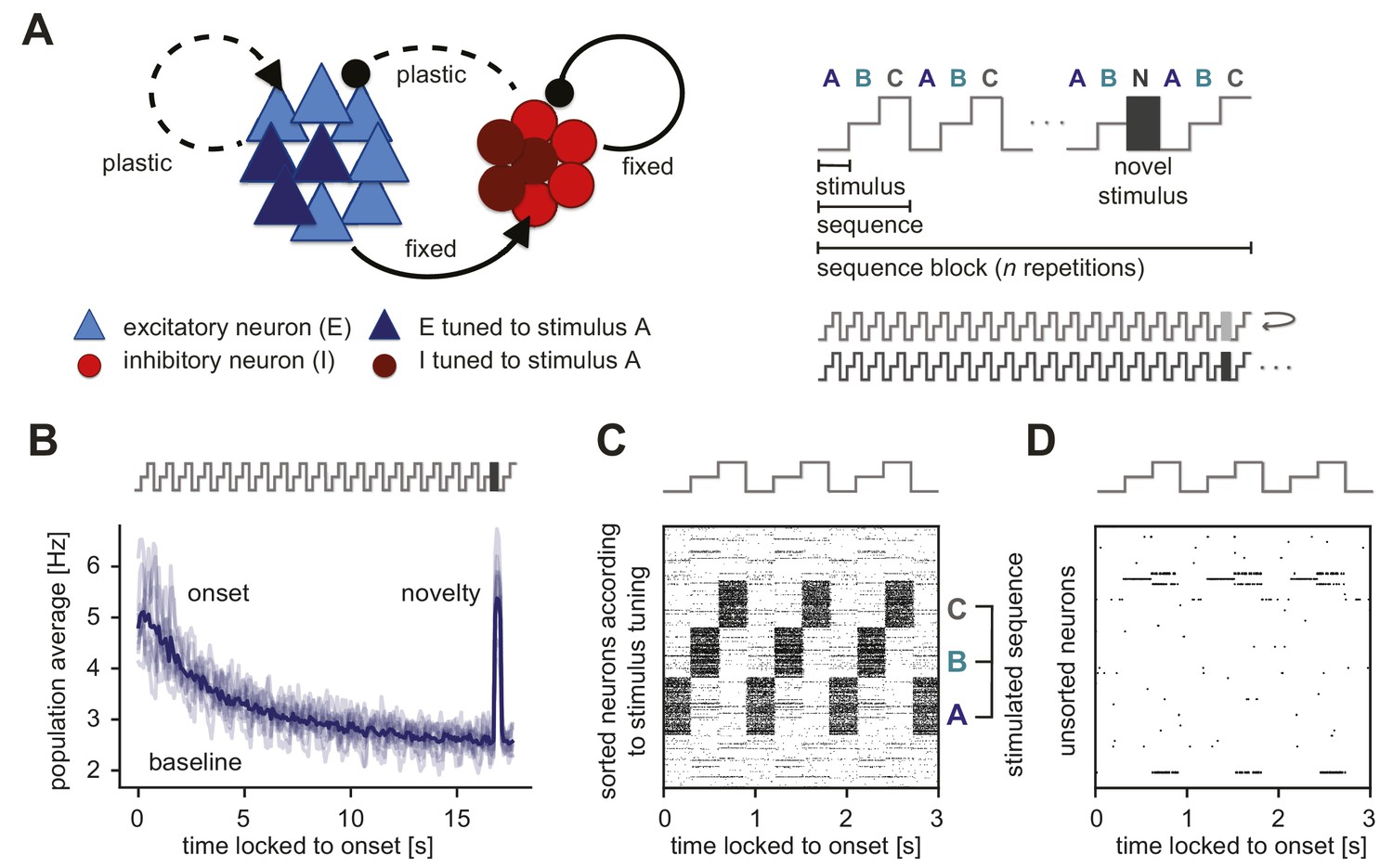
Generation of novelty responses in a recurrent plastic neural network model.
(A) Left: A recurrently connected network of excitatory (E) neurons (blue triangles) and inhibitory (I) neurons (red circles) receiving tuned input. Excitatory neurons tuned to a sample stimulus A are highlighted in dark blue, the inhibitory counterparts in dark red. E-to-E synapses and I-to-E synapses were plastic, and all other synapses were fixed. Right: Schematic of the stimulation protocol. Multiple stimuli (A, B, and C) were presented in a sequence (ABC). Each sequence was repeated times in a sequence block. In the second-to-last sequence, the last stimulus was replaced by a novel stimulus (N). Multiple sequence blocks followed each other without interruption, with each block containing sequences of different stimuli. (B) Population average firing rate of all excitatory neurons as a function of time after the onset of a sequence block. Activity was averaged (solid line) across multiple non-repeated sequence blocks (transparent lines: individual blocks). A novel stimulus (dark gray) was presented as the last stimulus of the second-to-last sequence. (C) Spiking activity in response to a sequence (ABC) in a subset of 1000 excitatory neurons where the neurons were sorted according to the stimulus from which they receive tuned input. A neuron can receive input from multiple stimuli and can appear more than once in this raster plot. (D) A random unsorted subset of 50 excitatory neurons from panel C. Time was locked to the sequence block onset.
Figure 1—figure supplement 1
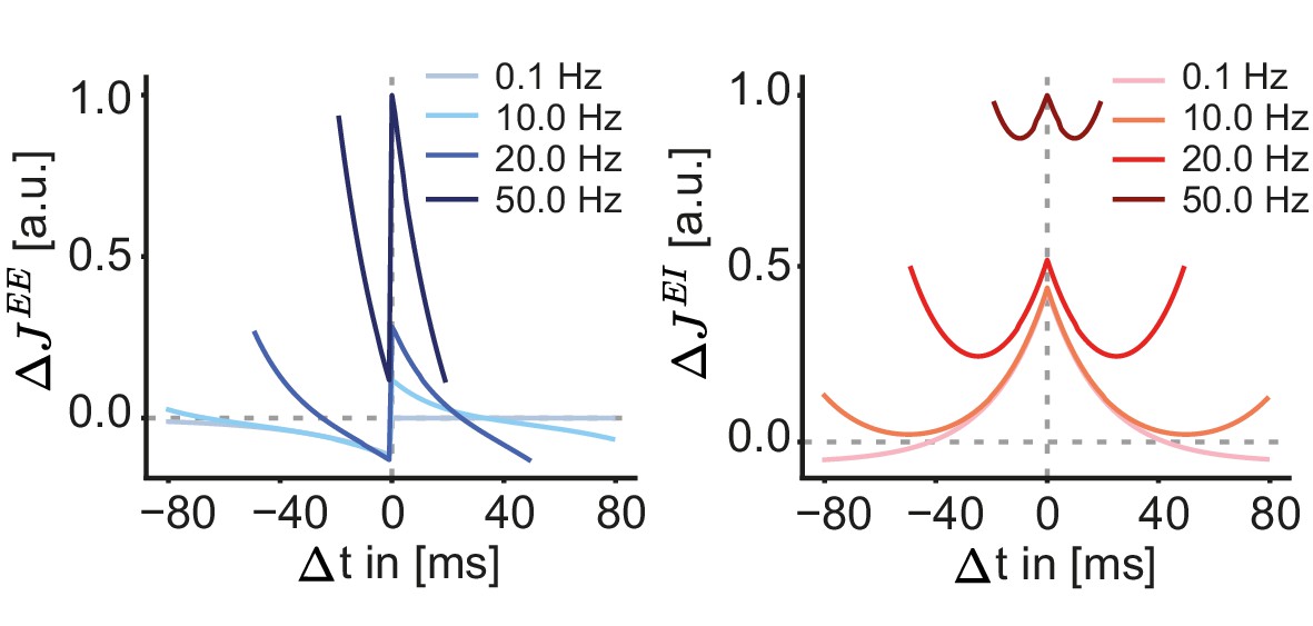
Excitatory and inhibitory synaptic plasticity functions for different pairing frequencies.
Synaptic weight change as a function of the time between pre- and postsynaptic spikes after the induction of 60 spike pairs at different pairing frequencies (0.1, 10, 20, and 50 Hz). Left: Triplet spike-timing-dependent plasticity rule of excitatory-to-excitatory connections . Right: Inhibitory spike-timing-dependent plasticity rule of inhibitory-to-excitatory connections .
Figure 1—figure supplement 2
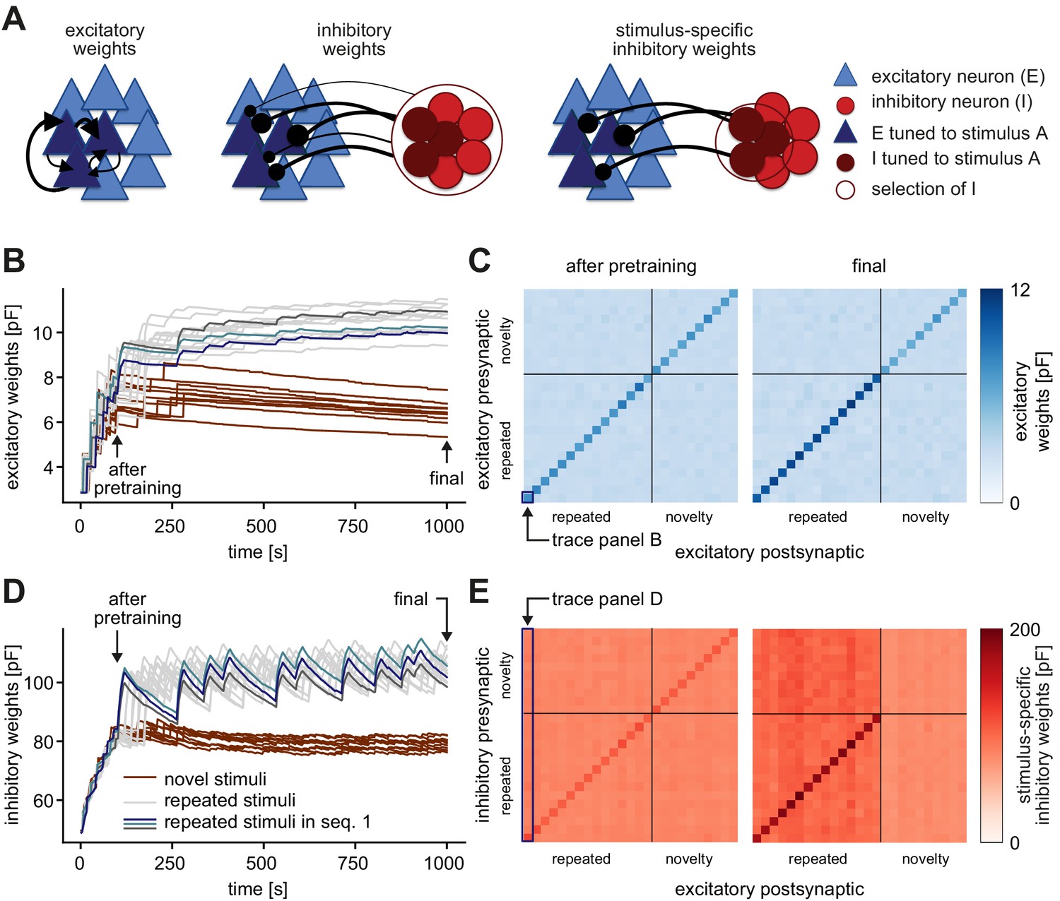
Strong connections form between excitatory and excitatory, as well as inhibitory and excitatory neuron groups that are tuned to the same stimulus.
(A) A recurrently connected network of excitatory (E) neurons (blue triangles) and inhibitory (I) neurons (red circles) receives tuned input. Excitatory neurons tuned to a sample stimulus A are highlighted in dark blue, the inhibitory counterparts in dark red. Left: Average excitatory weights within stimulus-specific assembly A are determined by averaging all E-to-E weights within an assembly. Center: Average inhibitory weights onto stimulus-specific assembly A are determined by averaging the weights from all inhibitory neurons onto stimulus-specific assembly A. Right: Stimulus-specific inhibitory weights onto stimulus-specific assembly A are determined by averaging only the weights from the inhibitory neurons that are also tuned to stimulus A (dark red). (B) Evolution of the average excitatory weights corresponding to all repeated and 10 sample novel stimuli. Colored traces mark three stimulus-specific assemblies in sequence 1: A, B, and C. The legend is shared with panel D. (C) Left: Weight matrix of average excitatory (E–to–E) weights after pretraining (see panel B) for all repeated and 10 sample novel stimuli separated by the gray lines. The size of assemblies can be slightly different. The weights across assemblies (off-diagonal) are small compared to the weights within assemblies (diagonal). After pretraining, there is no apparent difference in connectivity for novel and repeated stimuli. The diagonal elements correspond to the traces plotted in B, that is, the time evolution of the bottom-left square, highlighted in dark blue corresponds to the dark blue trace in panel B. Right: Same as left after the repeated sequence stimulation paradigm (see final in panel B). Here, assembly weights for repeated stimuli are stronger. (D) Same as panel B for the average inhibitory weights. Arrows indicate end points of the pretraining and whole stimulation phase. (E) Left: Weight matrix of stimulus-specific inhibitory (I–to–E) weights after pretraining (see panel D) for all repeated and 10 sample novel stimuli separated by the gray lines. The size of assemblies can be slightly different. Inhibition is stimulus-specific (diagonal stronger than off diagonal), that is, the weights from inhibitory neurons tuned to a given stimulus onto excitatory neurons that are tuned to the same stimulus (diagonal) are larger that onto excitatory neurons that are tuned to different stimuli (off-diagonal). After pretraining, there is no apparent difference in connectivity for novel and repeated stimuli. Here, an entire column average approximately corresponds to the traces plotted in D, that is, the time evolution of the averaged first column, highlighted in dark blue corresponds to the dark blue trace in panel D. It is only approximate, since individual inhibitory neurons can be tuned to multiple repeated and novel stimuli and hence contribute to multiple averages shown here in the matrix. Right: Same as left after the repeated sequence stimulation paradigm (see final in panel D). Here, excitatory assemblies tuned to repeated stimuli receive more inhibition than those tuned to novel stimuli.
Figure 1—figure supplement 3
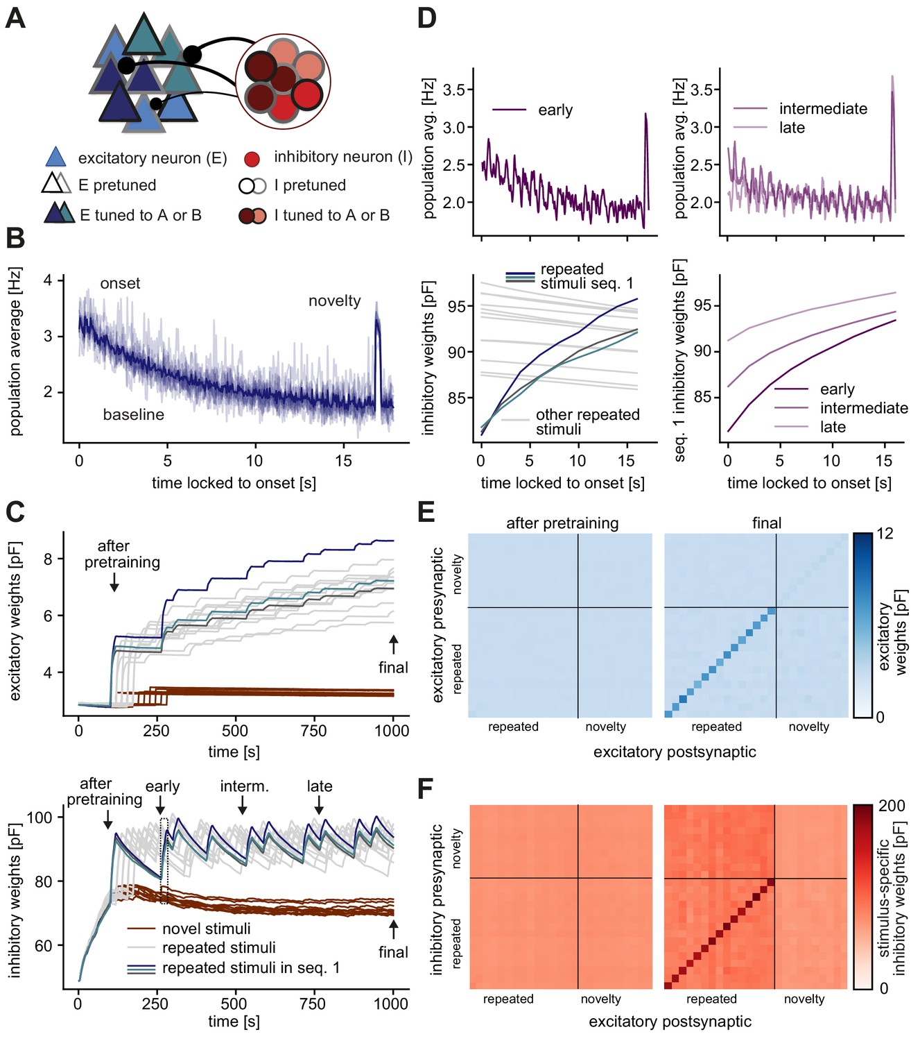
Different stimuli in the pretraining and stimulation phases generate similar synaptic weight and firing rate dynamics.
(A) Schematic of increased inhibitory weights onto stimulus-specific assemblies upon the repeated presentation of stimuli A and B (indicated by dark blue and turquoise) relative to neurons from other assemblies (light blue). Both, excitatory and inhibitory neurons were pretuned to different stimulus features (black and gray borders). (B) Population average firing rate of all excitatory neurons as a function of time after the onset of a sequence block. Activity was averaged (solid line) across multiple non-repeated sequence blocks (transparent lines: individual blocks). A novel stimulus was presented as the last stimulus of the second-to-last sequence. (C) Top: Evolution of the average excitatory weights corresponding to all repeated and 10 sample novel stimuli. Colored traces mark three stimulus-specific assemblies in sequence 1: A, B, and C. The legend is shared with bottom panel. Bottom: Same as top panel for the average inhibitory weights. Arrows indicate end points of the pretraining, early, intermediate and late time points and whole stimulation phase. (D) Top, left: Population average firing rate of all excitatory neurons during the repeated presentation of sequence 1 at an early time point (see panel C, bottom). The novelty response can be seen at the end of the stimulation period. Bottom, left: Close-up of panel C, bottom (rectangle). Top, right: Same as panel top, left but at intermediate and late time points (see panel C, bottom). Bottom, right: Corresponding dynamics of the average inhibitory weights onto all three stimulus-specific assemblies from sequence 1 at early, intermediate and late time points (see panel C, bottom). The dark purple trace (early) corresponds to the average of the three colored traces in bottom, left panel. Time is locked to sequence onset. (E) Left: Weight matrix of average excitatory (E–to–E) weights after pretraining (see panel C), sorted by repeated and novel stimuli (repeated and novel stimuli are separated by the black lines). Right: Same as left after the repeated sequence stimulation paradigm (see final in panel C, top). The diagonal elements correspond to the traces plotted in C, top. (F) Left: Weight matrix of stimulus-specific inhibitory (I–to–E) weights after pretraining (see panel C, bottom), sorted by repeated and novel stimuli (repeated and novel stimuli are separated by the black lines). Right: Same as left after the repeated sequence stimulation paradigm (see final in panel C,bottom). .
Figure 1—figure supplement 4
Quantifying response density in the unique sequence stimulation paradigm.
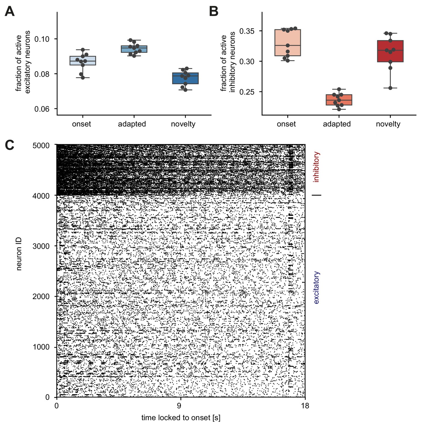
Single neuron statistics measured for 100 ms directly after the onset of the stimulus (onset), after the onset of the novel stimulus (novelty) and shortly before the novel stimulus is presented (adapted). (A) Fraction of active excitatory neurons (at least one spike in a 100 ms window) for the three different time-points of the stimulation paradigm. Horizontal line indicates the median, boxes are drawn between the 25th and 75th percentile, whiskers extend above and below the box to the most extreme data points that are within a distance to the box equal to 1.5 times the interquartile range and points indicate all data points. Each data point corresponds to a unique sequence block. (B) Same as A for inhibitory neurons. (C) Spike raster of all neurons sorted according to neuron ID during one sequence block. Time is locked to sequence block onset.
Figure 1—figure supplement 5
Normalization time step does not affect the occurrence of a novelty response.
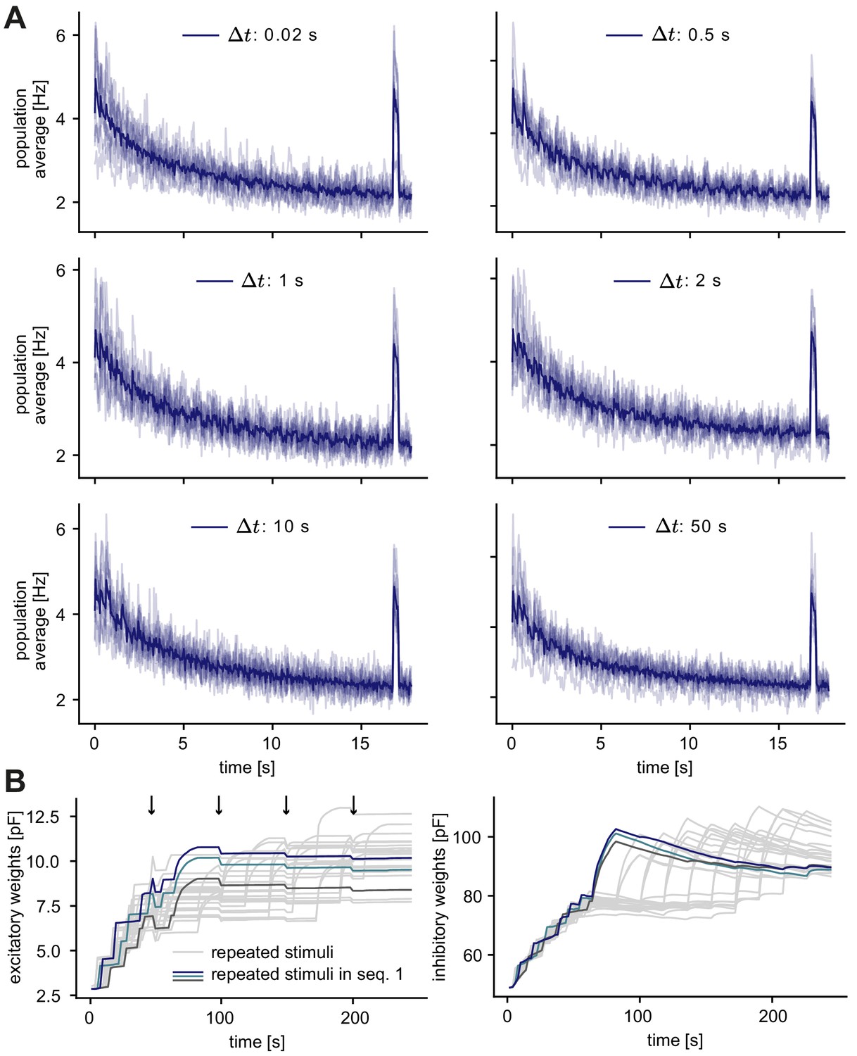
(A) Population average firing rate of all excitatory neurons as a function of time after the onset of a sequence block for different normalization time steps . Activity was averaged (solid line) across multiple non-repeated sequence blocks (transparent lines: individual blocks). A novel stimulus was presented as the last stimulus of the second-to-last sequence. (B) Left: Evolution of the average excitatory weights corresponding to 10 repeated stimuli with . Arrows indicate the time-point of normalization. Colored traces mark three stimulus-specific assemblies in sequence 1: A, B, and C. Right: Same as left panel for the average inhibitory weights.
Figure 2

Dependence of the novelty response on the number of sequence repetitions and the sequence length.
(A) Population average firing rate of all excitatory neurons for a different number of sequence repetitions within a sequence block. Time is locked to the sequence block onset. (B) The response amplitude of the onset (gray) and the novelty (black) response as a function of sequence repetitions fit with an exponential with a time constant . (C) Population average firing rate of all excitatory neurons for varying sequence length fit with an exponential function (red). Time is locked to the sequence block onset. (D) The onset decay time constant (fit with an exponential, as shown in panel C) as a function of sequence length. The simulated data was fit with a linear function with slope . (B, D) Error bars correspond to the standard deviation across five simulated instances of the model.
Figure 3
Stimulus periodicity in the sequence is not required for the generation of a novelty response.
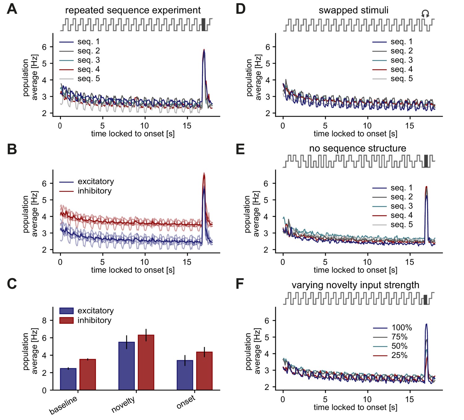
(A–F) Population average firing rate of all excitatory neurons (and all inhibitory neurons in B,C) during the presentation of five different repeated sequence blocks. The population firing rate was averaged across ten repetitions of each sequence block. Time is locked to sequence block onset. (A) A novel stimulus was presented as the last stimulus of the second-to-last sequence. (B) Same as panel A but for both excitatory and inhibitory populations (transparent lines: individual sequence averages). (C) Comparison of baseline, novelty, and onset response for inhibitory and excitatory populations. Error bars correspond to the standard deviation across the five sequence block averages shown in B. (D) In the second-to-last sequence, the last and second-to-last stimulus were swapped instead of presenting a novel stimulus. (E) Within a sequence, stimuli were shuffled in a pseudo-random manner where a stimulus could not be presented twice in a row. A novel stimulus was presented as the last stimulus of the second-to-last sequence. (F) A novel stimulus was presented as the last stimulus of the second-to-last sequence. Each sequence had a different feedforward input drive for the novel stimulus, indicated by the percentage of the typical input drive for the novel stimulus used before.
Figure 4 with 2 supplements
Inhibition onto neurons tuned to repeated stimuli increases during sequence repetitions.
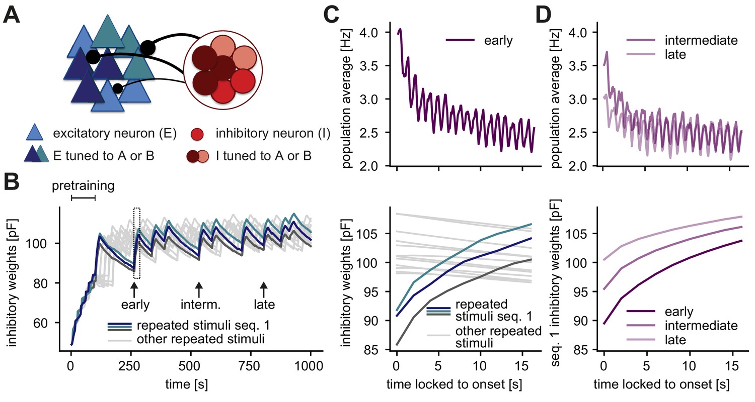
(A) Schematic of increased inhibitory weights onto two stimulus-specific assemblies upon the repeated presentation of stimuli A and B (indicated in dark blue and turquoise) relative to neurons from other assemblies (light blue). (B) Evolution of the average inhibitory weights onto stimulus-specific assemblies. Colored traces mark three stimulus-specific assemblies in sequence 1: A, B, and C. Arrows indicate time points of early, intermediate, and late sequence block presentation shown in C and D. (C) Top: Population average firing rate of all excitatory neurons during the repeated presentation of sequence 1 at an early time point (see panel B). Time is locked to sequence onset. Bottom: Close-up of panel B (rectangle). Time is locked to sequence onset. (D) Top: Same as panel C (top) but at intermediate and late time points (see panel B). Bottom: Corresponding dynamics of the average inhibitory weights onto all three stimulus-specific assemblies from sequence 1 at early, intermediate and late time points (see panel B). The dark purple trace (early) corresponds to the average of the three colored traces in C (bottom).
Figure 4—figure supplement 1
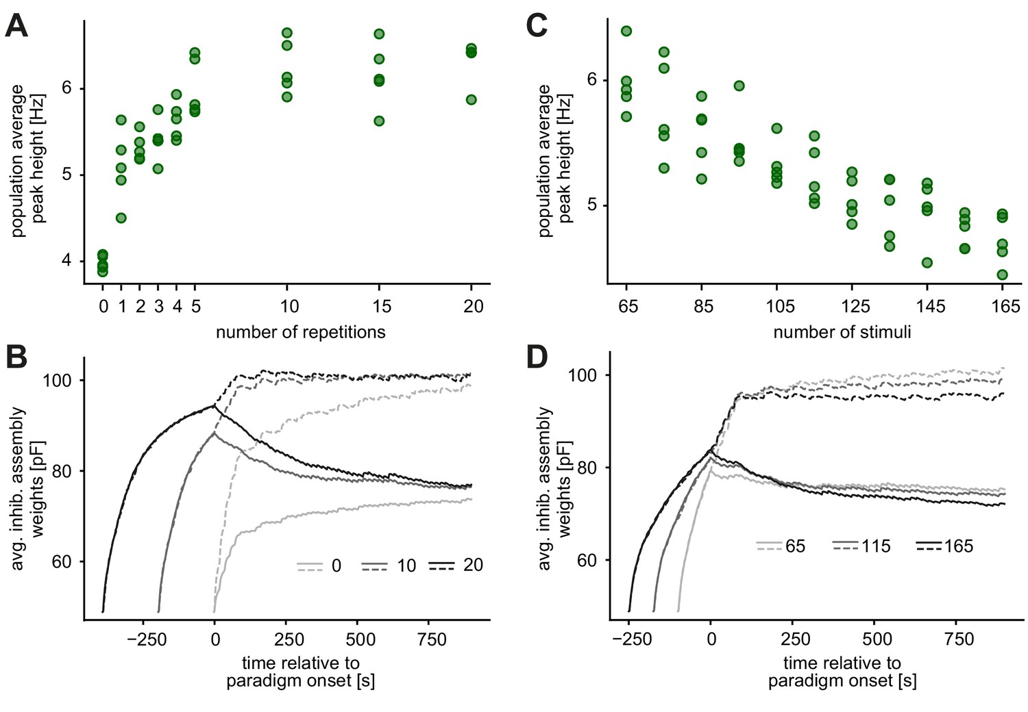
Pretraining parameters do not qualitatively influence the novelty response.
(A) The novelty peak height as a function of the number of repetitions. The same 65 stimuli were presented during the pretraining and the consecutive stimulation paradigm (paradigm stimuli). (B) Evolution of the average inhibitory weights onto all stimulus-specific assemblies of repeated (full line) or novel (dashed line) stimuli. Shades of gray represent the average inhibitory weights for different number of repetitions of each stimulus. (C) The novelty peak height as a function of the total number of stimuli in the pretraining phase. Each of the 65 paradigm stimuli and (0 to 100) additional stimuli are repeated five times during pretraining. (D) Same as panel B, where now shades of gray represent the average inhibitory weights for different number of stimuli.
Figure 4—figure supplement 2
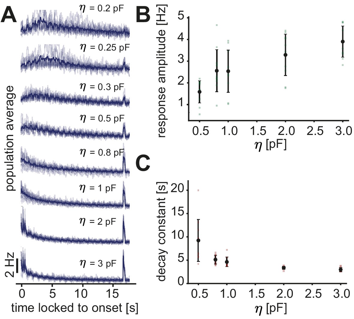
Fast inhibitory plasticity is key for the generation of a novelty response.
(A) Population average firing rate of all excitatory neurons as a function of time after the onset of a sequence block. Activity was averaged (solid line) across multiple non-repeated sequence blocks (transparent lines: individual blocks). A novel stimulus was presented as the last stimulus of the second-to-last sequence. Each panel shows the population average for a different inhibitory learning rate . For reference, we use in the remaining of the manuscript. (B) The response amplitude of the novelty response as a function of the inhibitory learning rate . (C) The onset decay time constant (fit with an exponential) as a function of the inhibitory learning rate . Error bars correspond to the standard deviation, dots are results from a single run.
Figure 5
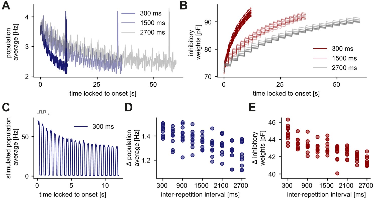
Longer inter-repetition intervals decrease the level of adaptation due to the recovery of inhibitory synaptic weights.
(A) Population average firing rate of all excitatory neurons in the unique sequence stimulation paradigm for varying inter-repetition intervals (varying sequence length). Time is locked to the sequence block onset. (B) Evolution of the average inhibitory weights onto stimulus-specific assembly A (identical in all runs) for varying inter-repetition intervals. Time is locked to the sequence block onset. (C) Population average firing rate of stimulated excitatory neurons for a 300 ms inter-repetition interval. Time is locked to the sequence block onset. One step in the schematic corresponds to one stimulus in a presented sequence. (D) Difference of the onset population rate (measured at the onset of the stimulation, averaged across runs) and the baseline rate (measured before novelty response) as a function of the inter-repetition interval. (E) Absolute change of inhibitory weights onto stimulus-specific assembly A from the start until the end of a sequence block presentation as a function of inter-repetition interval.
Figure 6 with 1 supplement
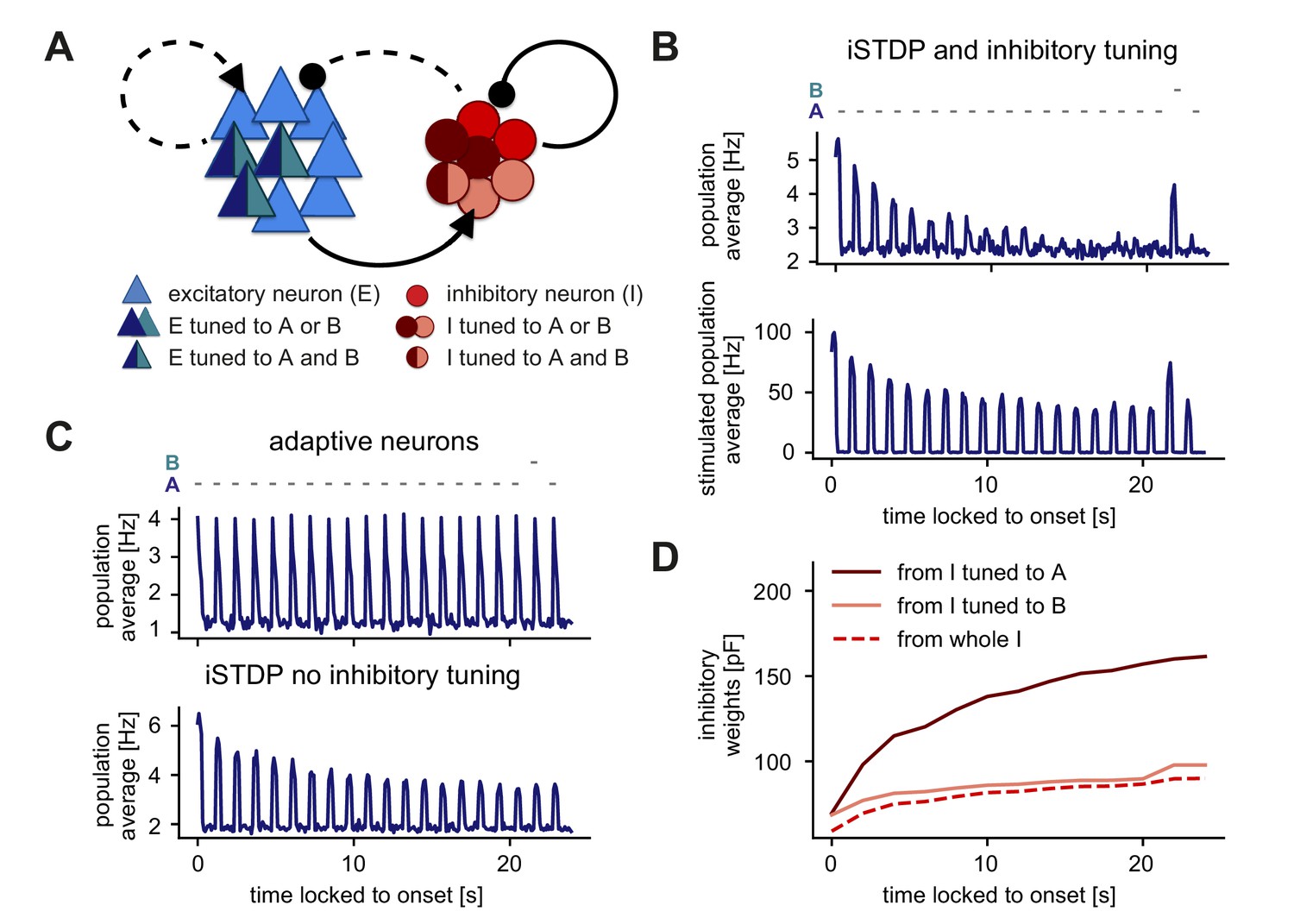
Stimulus-specific adaptation follows from inhibitory plasticity and tuning of both excitatory and inhibitory neurons.
(A) Stimuli A and B provided input to the same excitatory neurons (dark blue and turquoise). Some neurons in the inhibitory population were driven by both A and B (dark red and rose) and some by only one of the two stimuli (dark red or rose). (B,C) Population average firing rate of excitatory neurons over time while stimulus A was presented 20 times. Stimulus B was presented instead of A as the second-to-last stimulus. Time is locked to stimulation onset. (B) Top: Population average of all excitatory neurons in the network with inhibitory plasticity (iSTDP) and inhibitory tuning. Bottom: Population average of stimulated excitatory neurons only (stimulus-specific to A and B). (C) Top: Same as panel B (top) for neurons with an adaptive current in a non-plastic recurrent network. Bottom: Same as panel B (top) for the network with inhibitory plasticity (iSTDP) and no inhibitory tuning. (D) Weight evolution of stimulus-specific inhibitory weights corresponding to stimuli A and B and average inhibitory weights.
Figure 6—figure supplement 1
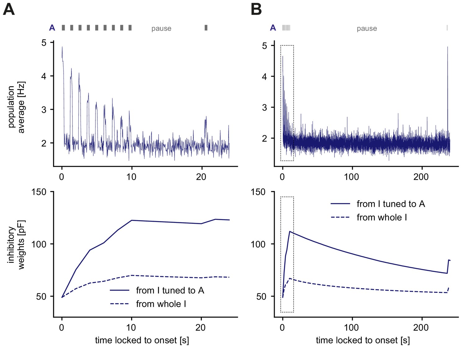
Recovery of adapted responses in the SSA paradigm.
The stimulus is shown nine times while the population response adapts. This is followed by a long pause, and then the same stimulus is shown once more. The inter-stimulus interval here is 900 ms, while stimuli are presented for 300 ms. (A) Population average of all excitatory neurons during repeated presentation of stimulus A followed by a short pause (9 s) and then another presentation of A (top). Weight evolution of stimulus-specific inhibitory weights during the stimulation paradigm (bottom). Time is locked to stimulus onset. (B) Same as A but with a much longer pause (225 s). The initial stimulation paradigm in panel A is the same as in panel B (indicated with the box).
Figure 7
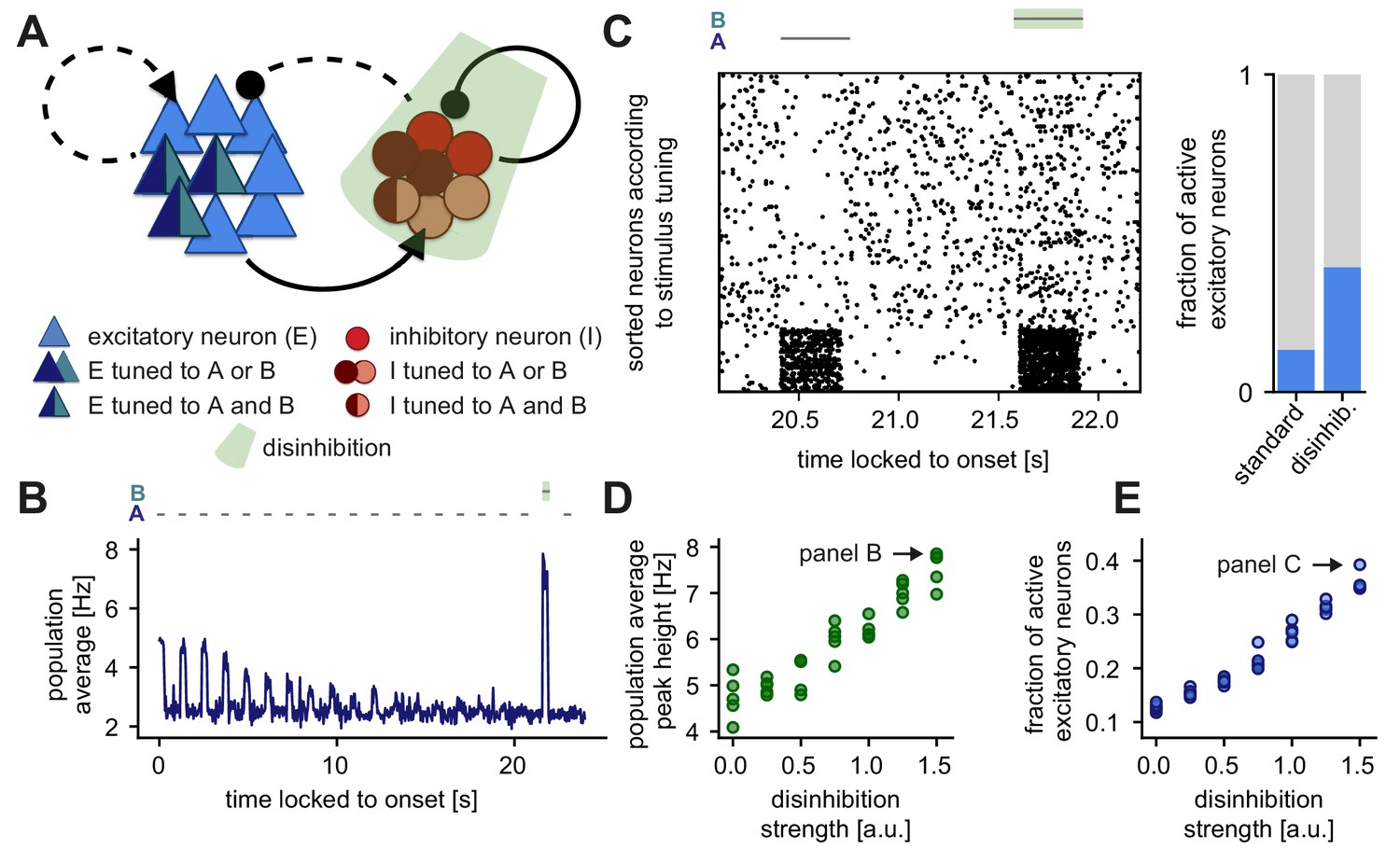
Disinhibition leads to a novelty response amplification and a dense population response.
(A) Stimuli A and B provided input to the same excitatory neurons (dark blue and turquoise). Some neurons in the inhibitory population were driven by both A and B (dark red and rose) and some by only one of the two stimuli (dark red or rose). Inhibition (light green) of the entire inhibitory population led to disinhibition of the excitatory population. (B) Population average firing rate of all excitatory neurons over time while stimulus A is presented 20 times. Stimulus B was presented instead of A as the second-to-last stimulus. During the presentation of B, the inhibitory population was inhibited. Time is locked to stimulation onset. (C) Left: Raster plot of 250 excitatory neurons corresponding to the population average shown in panel B. The 50 neurons in the bottom part of the raster plot were tuned to stimuli A and B. Time is locked to stimulation onset. Right: Fraction of active excitatory neurons (at least one spike in a 100 ms window) measured directly after the onset of a stimulus. The raster plot and the fraction of active excitatory neurons are shown for the presentation of stimulus B (with disinhibition) and the preceding presentation of stimulus A (standard). (D) Population average peak height during disinhibition and the presentation of stimulus B, as a function of the disinhibition strength. Arrow indicates the population average peak height of the trace shown in panel B. Results are shown for five simulations. (E) Fraction of active excitatory neurons during disinhibition as a function of the disinhibition strength. Arrow indicates the data point corresponding to panel C. Results are shown for five simulations.
Author response image 1

Disinhibiting the standard and deviant stimulus leads to differential increase in responses to standard and deviant tones.
A. Population firing rate of excitatory neurons in response to standard stimuli (gray) or to deviant stimuli (red) without disinhibition (dark colors) and with disinhibition (suppression of the total inhibitory population) (light colors). All responses are normalized to the response to the fourth non-disinhibited post-novelty stimulus of one instantiation of the model. B. Difference between firing rates with and without disinhibition from panel A in response to standard (gray) and deviant (red) stimuli. Error bars correspond to the standard deviation across three model instantiations.
Tables
Table 1
Parameters for the excitatory (EIF) and inhibitory (LIF) membrane dynamics (Litwin-Kumar and Doiron, 2014).
| Symbol | Description | Value |
|---|---|---|
| Number of E neurons | 4000 | |
| Number of I neurons | 1000 | |
| , | E, I neuron resting membrane time constant | 20 ms |
| E neuron resting potential | - 70 mV | |
| I neuron resting potential | - 62 mV | |
| Slope factor of exponential | 2 mV | |
| Membrane capacitance | 300 pF | |
| Membrane conductance | C/ | |
| E reversal potential | 0 mV | |
| I reversal potential | - 75 mV | |
| Threshold potential | - 52 mV | |
| Peak threshold potential | 20 mV | |
| E, I neuron reset potential | - 60 mV | |
| E, I absolute refractory period | 1 ms |
Table 2
Parameters for feedforward and recurrent connections (Litwin-Kumar and Doiron, 2014).
| Symbol | Description | Value |
|---|---|---|
| Connection probability | 0.2 | |
| Rise time for E synapses | 1 ms | |
| Decay time for E synapses | 6 ms | |
| Rise time for I synapses | 0.5 ms | |
| Decay time for I synapses | 2 ms | |
| Avg. rate of external input to E neurons | 4.5 kHz | |
| Avg. rate of external input to I neurons | 2.25 kHz | |
| Minimum E to E synaptic weight | 1.78 pF | |
| Maximum E to E synaptic weight | 21.4 pF | |
| Initial E to E synaptic weight | 2.76 pF | |
| Minimum I to E synaptic weight | 48.7 pF | |
| Maximum I to E synaptic weight | 243 pF | |
| Initial I to E synaptic weight | 48.7 pF | |
| Synaptic weight from E to I | 1.27 pF | |
| Synaptic weight from I to I | 16.2 pF | |
| Synaptic weight from external input population to E | 1.78 pF | |
| Synaptic weight from external input population to I | 1.27 pF |
Table 3
Parameters for the implementation of Hebbian and homeostatic plasticity (Pfister and Gerstner, 2006; Litwin-Kumar and Doiron, 2014).
| Symbol | Description | Value |
|---|---|---|
| Time constant of pairwise pre-synaptic detector (+) | 33.7 ms | |
| Time constant of pairwise post-synaptic detector (-) | 16.8 ms | |
| Time constant of triplet pre-synaptic detector (-) | 101 ms | |
| Time constant of triplet post-synaptic detector (+) | 125 ms | |
| Pairwise potentiation amplitude | pF | |
| Triplet potentiation amplitude | pF | |
| Pairwise depression amplitude | pF | |
| Triplet depression amplitude | pF | |
| Time constant of low-pass filtered spike train | 20 ms | |
| Inhibitory plasticity learning rate | 1 pF | |
| Target firing rate | 3 Hz |
Table 4
Parameters for the stimulation paradigm and stimulus tuning.
| Symbol | Description | Value |
|---|---|---|
| External baseline input to E | 4.5 kHz | |
| External baseline input to I | 2.25 kHz | |
| Additional input to E during stimulus presentation | 12 kHz | |
| Additional input to I during stimulus presentation | 1.2 kHz | |
| Additional input to I during disinhibition | −1.5 kHz | |
| Probability for an E neuron to be driven by a stimulus | 5% | |
| Probability for an I neuron to be driven by a stimulus | 15% |
Additional files
Download links
A two-part list of links to download the article, or parts of the article, in various formats.
Downloads (link to download the article as PDF)
Open citations (links to open the citations from this article in various online reference manager services)
Cite this article (links to download the citations from this article in formats compatible with various reference manager tools)
The generation of cortical novelty responses through inhibitory plasticity
eLife 10:e65309.
https://doi.org/10.7554/eLife.65309


