Creating and controlling visual environments using BonVision
- NeuroGEARS Ltd., United Kingdom
- UCL Institute of Behavioural Neuroscience, Department of Experimental Psychology, University College London, United Kingdom
Figures
Figure 1 with 2 supplements
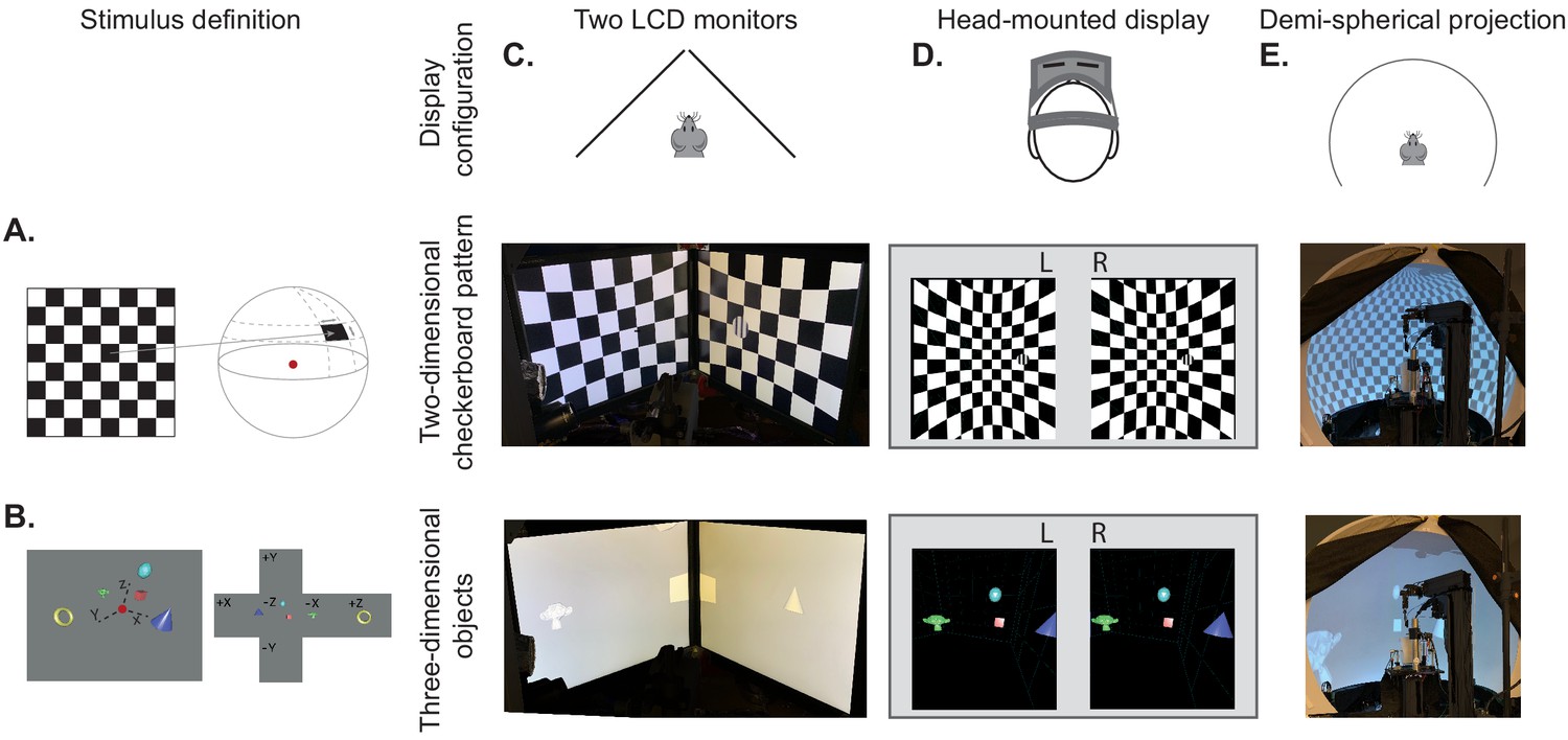
BonVision's adaptable display and render configurations.
(A) Illustration of how two-dimensional textures are generated in BonVision using Mercator projection for sphere mapping, with elevation as latitude and azimuth as longitude. The red dot indicates the position of the observer. (B) Three-dimensional objects were placed at the appropriate positions and the visual environment was rendered using cube-mapping. (C–E) Examples of the same two stimuli, a checkerboard + grating (middle row) or four three-dimensional objects (bottom row), displayed in different experimental configurations (top row): two angled LCD monitors (C), a head-mounted display (D), and demi-spherical dome (E).
Figure 1—figure supplement 1
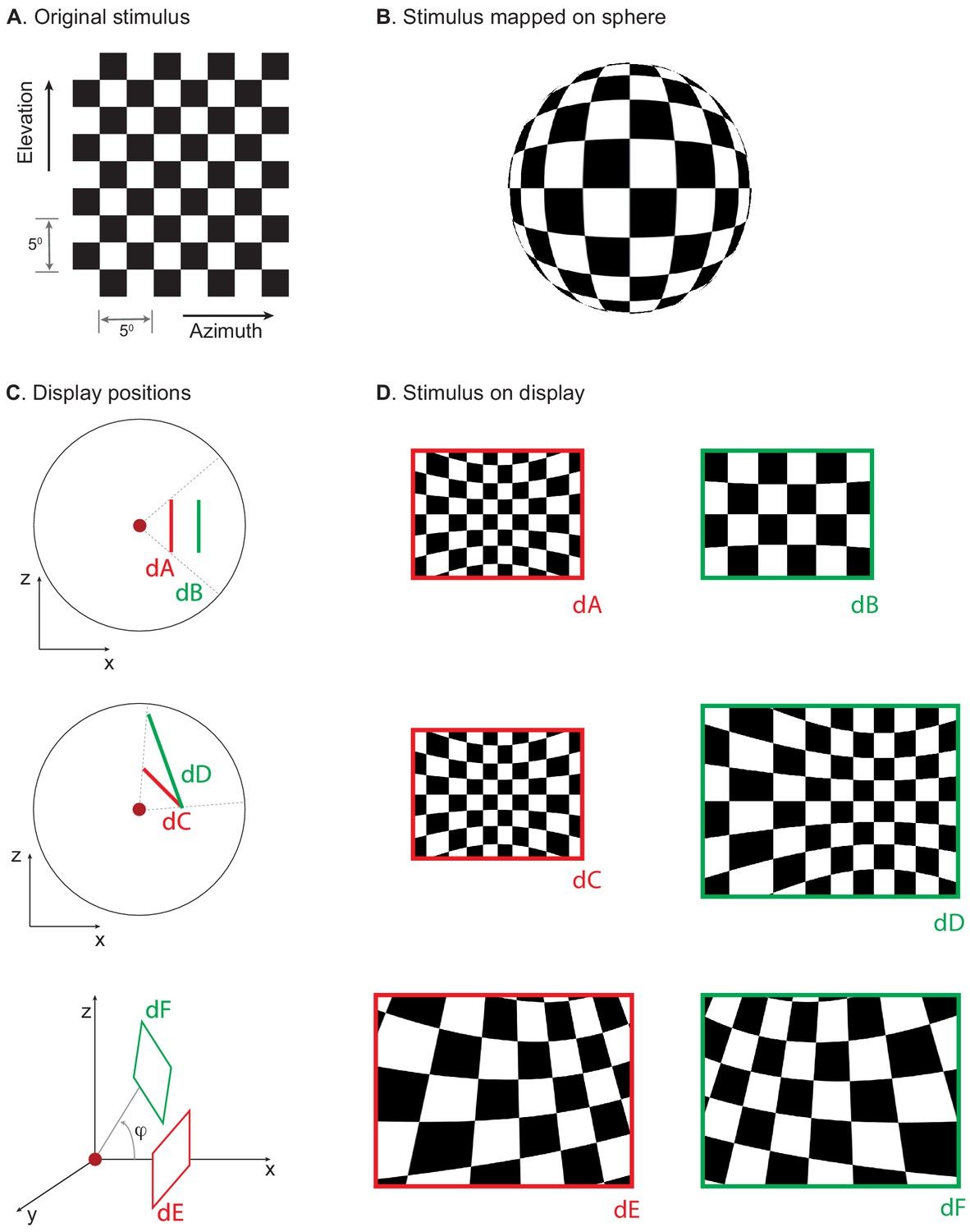
Mapping stimuli onto displays in various positions.
(A) Checkerboard stimulus being rendered. (B) Projection of the stimulus onto a sphere using Mercator projection. (C) Example display positions (dA–dF) and (D) corresponding rendered images. Red dot in C indicates the observer position.
Figure 1—figure supplement 2
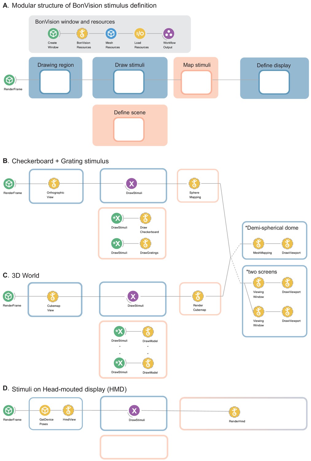
Modular structure of workflow and example workflows.
(A) Description of the modules in BonVision workflows that generate stimuli. Every BonVision stimuli includes a module that creates and initialises the render window, shown in ‘BonVision window and resources’. This defines the window parameters in Create Window (such as background colour, screen index, VSync), and loads predefined (BonVision Resources) and user defined textures (Texture Resources, not shown), and 3D meshes (Mesh Resources). This is followed by the modules: ‘Drawing region’, where the visual space covered by the stimuli is defined, which can be the complete visual space, 360° × 360°. ‘Draw stimuli’ and ‘Define scene’ are where the stimulus is defined, ‘Map Stimuli’, which maps the stimuli into the 3D environment, and ‘Define display’, where the display devices are defined. (B and C) Modules that define the checkerboard +grating stimulus (B) shown in the middle row of Figure 1 and 3D world (C) with five objects shown in the bottom row of Figure 1. The display device is defined separately and either display can be appended at the end of the workflow. This separation of the display device allows for replication between experimental configurations. (D) The variants of the modules used to display stimuli on a head-mounted display. The empty region under ‘Define scene’ would be filled by the corresponding nodes in B and C.
Figure 2 with 2 supplements
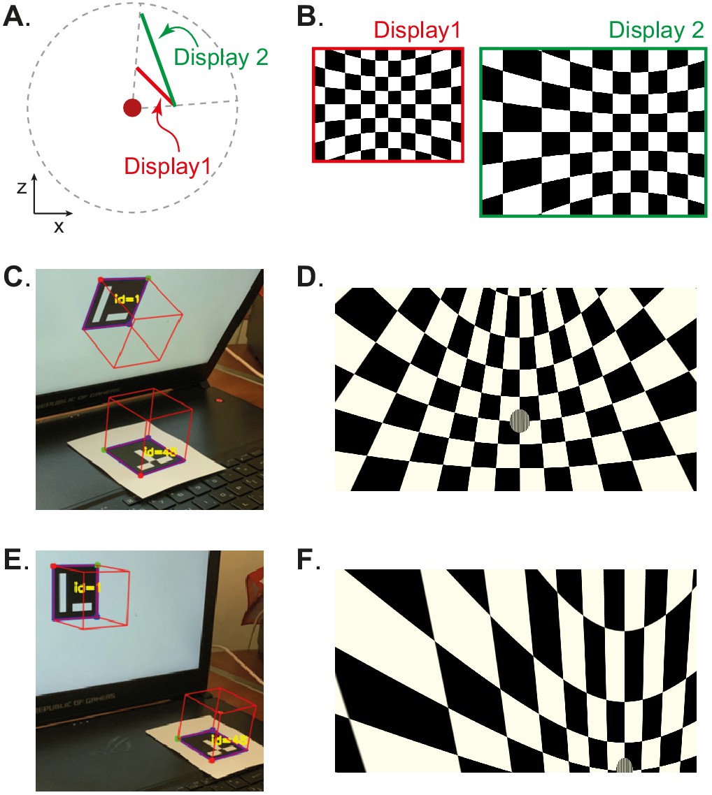
Automated calibration of display position.
(A) Schematic showing the position of two hypothetical displays of different sizes, at different distances and orientation relative to the observer (red dot). (B) How a checkerboard of the same visual angle would appear on each of the two displays. (C) Example of automatic calibration of display position. Standard markers are presented on the display, or in the environment, to allow automated detection of the position and orientation of both the display and the observer. These positions and orientations are indicated by the superimposed red cubes as calculated by BonVision. (D) How the checkerboard would appear on the display when rendered, taking into account the precise position of the display. (E and F) Same as (C and D), but for another pair of display and observer positions. The automated calibration was based on the images shown in C and E.
Figure 2—figure supplement 1
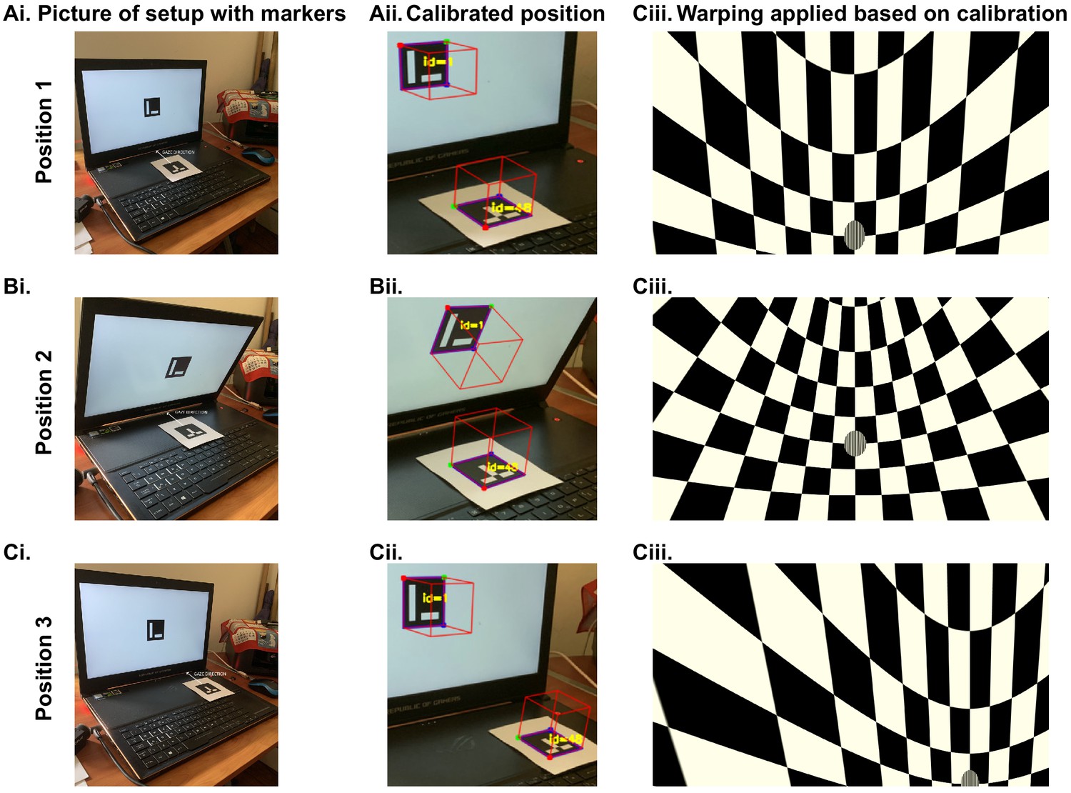
Automated workflow to calibrate display position.
The automated calibration is carried out by taking advantage of ArUco markers (Del Grosso and Sirota, 2019) that can be used to calculate the 3D position of a surface. (Ai) We use one marker on the display and one placed in the position of the observer. We then use a picture of the display and observer position taken by a calibrated camera. This is an example where we used a mobile phone camera for calibration. (Aii) The detected 3D positions of the screen and the observer, as calculated by BonVision. (Aiii) A checkerboard image and a small superimposed patch of grating, rendered based on the precise position of the display. (B and C) same as A and C for different screen and observer positions: with the screen tilted towards the animal (B), or the observer shifted to the right of the screen (C). The automated calibration was based on the images shown in Ai, Bi, and Ci, which in this case were taken using a mobile phone camera.
Figure 2—figure supplement 2
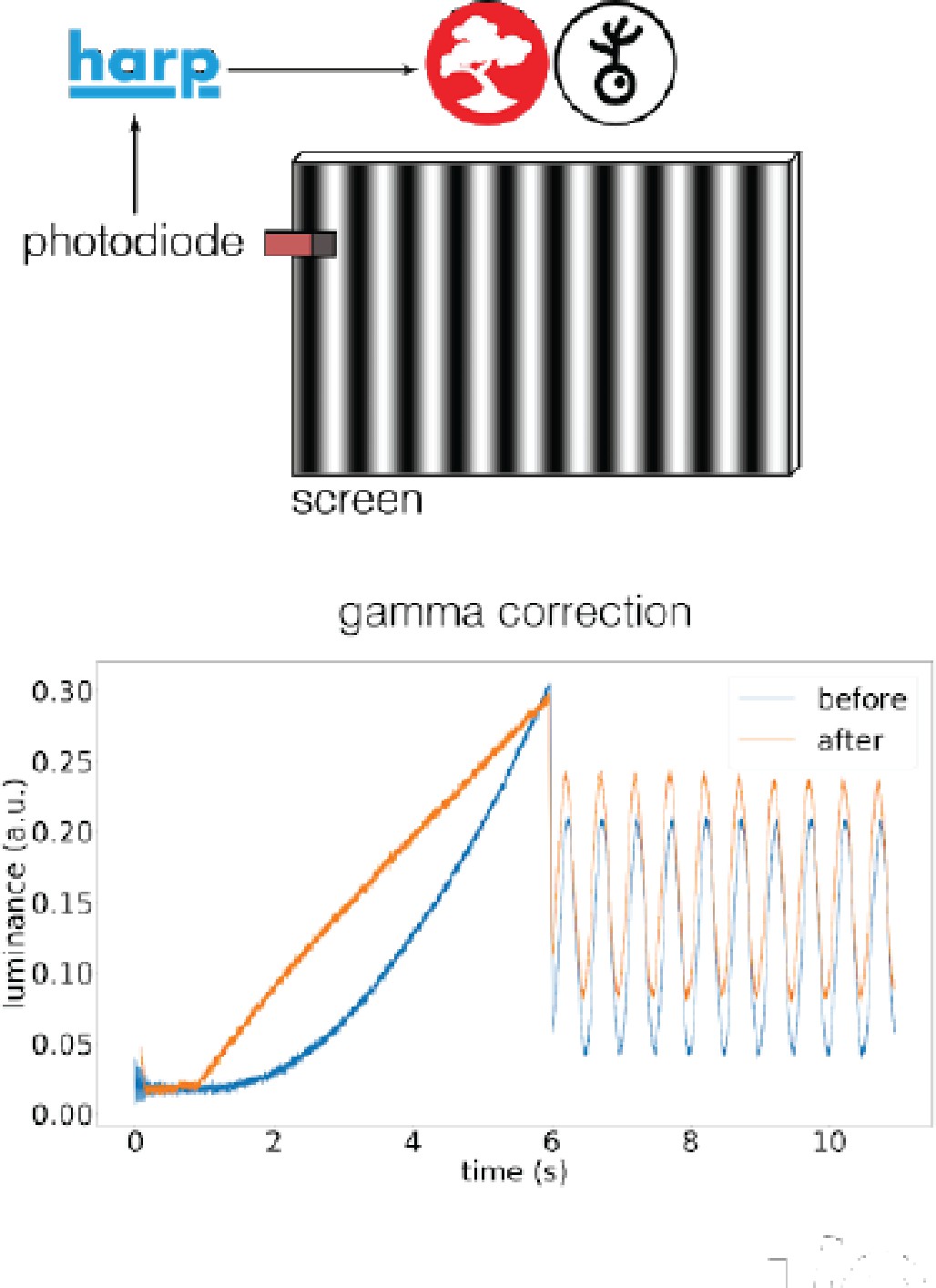
Automated gamma-calibration of visual displays.
BonVision monitored a photodiode (Photodiode v2.1, https://www.cf-hw.org/harp/behavior) through a HARP microprocessor to measure the light output of the monitor (Dell Latitude 7480). The red, green, and blue channels of the display were sent the same values (i.e. grey scale). (A) Gamma calibration. The input to the display channels was modulated by a linear ramp (range 0–255). Without calibration the monitor output (arbitrary units) increased exponentially (blue line). The measurement was then used to construct an intermediate look-up table that corrected the values sent to the display. Following calibration, the display intensity is close to linear (red line). Inset at top: schematic of the experimental configuration. (B) Similar to A, but showing the intensity profile of a drifting sinusoidal grating. Measurements before calibration resemble an exponentiated sinusoid (blue dotted line). Measurements after calibration resemble a regular sinusoid (red dotted line).
Figure 3 with 1 supplement
Using BonVision to generate an augmented reality environment.
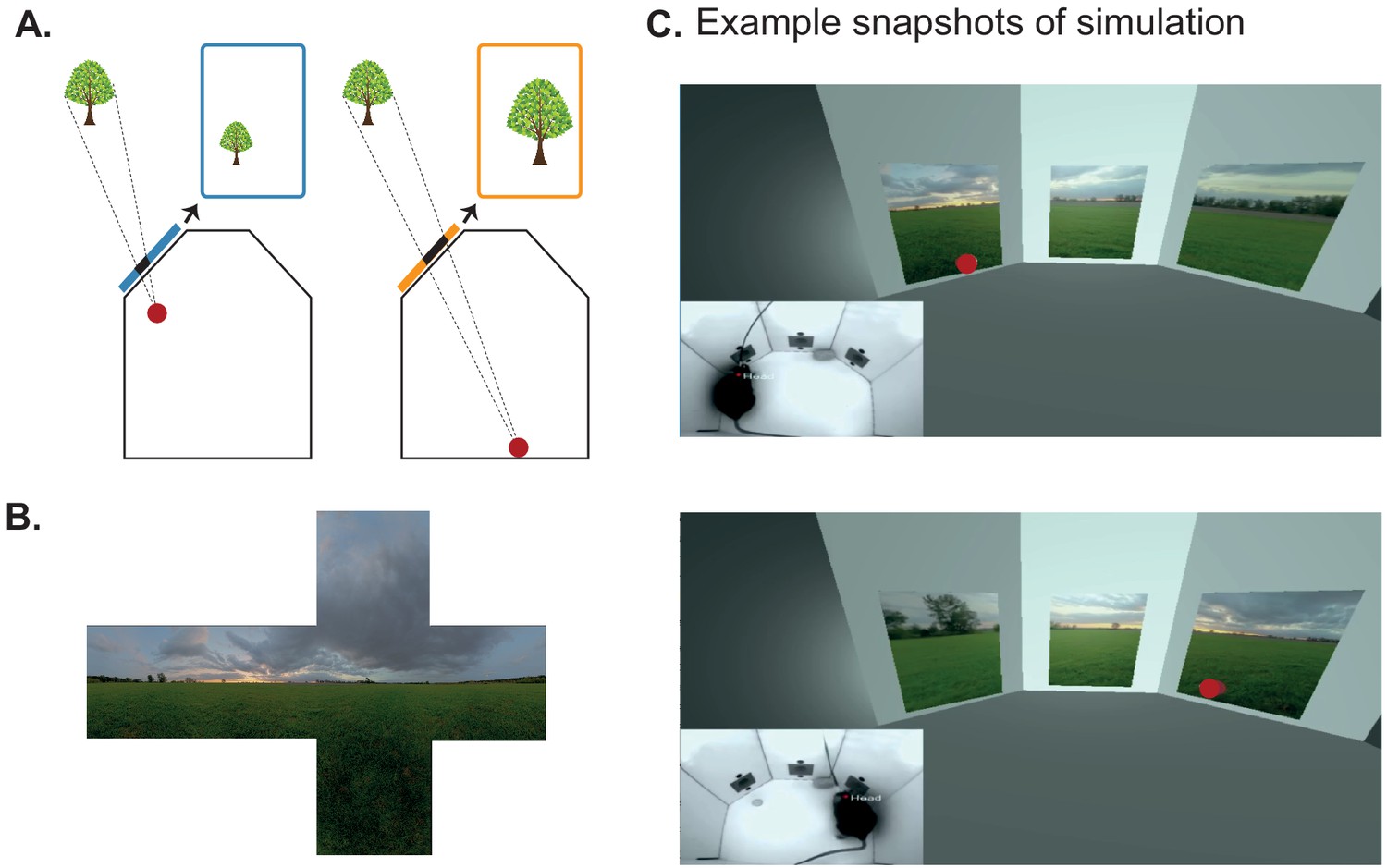
(A) Illustration of how the image on a fixed display needs to adapt as an observer (red dot) moves around an environment. The displays simulate windows from a box into a virtual world outside. (B) The virtual scene (from: http://scmapdb.com/wad:skybox-skies) that was used to generate the example images and Figure 3—video 1 offline. (C) Real-time simulation of scene rendering in augmented reality. We show two snapshots of the simulated scene rendering, which is also shown in Figure 3—video 1. In each case the inset image shows the actual video images, of a mouse exploring an arena, that were used to determine the viewpoint of an observer in the simulation. The mouse’s head position was inferred (at a rate of 40 frames/s) by a network trained using DeepLabCut (Aronov and Tank, 2014). The top image shows an instance when the animal was on the left of the arena (head position indicated by the red dot in the main panel) and the lower image shows an instance when it was on the right of the arena.
Figure 3—video 1
Augmented reality simulation using BonVision.
This video is an example of a deep neural network, trained with DeepLabCut, being used to estimate the position of a mouse’s head in an environment in real-time, and updating a virtual scene presented on the monitors based on this estimated position. The first few seconds of the video display the online tracking of specific features (nose, head, and base of tail) while an animal is moving around (shown as a red dot) in a three-port box (as in Soares et al., 2016). Subsequently the inset shows the original video of the animal’s movements, which the simulation is based on. The rest of the video image shows how a green field landscape (source: http://scmapdb.com/wad:skybox-skies) outside the box would be rendered on three simulated displays within the box (one placed on each of the three oblique walls). These three displays simulate windows onto the world beyond the box. The position of the animal was updated by DeepLabCut at 40 frames/s, and the simulation was rendered at the same rate.
Figure 4 with 1 supplement
Closed-loop latency and performance benchmarks.
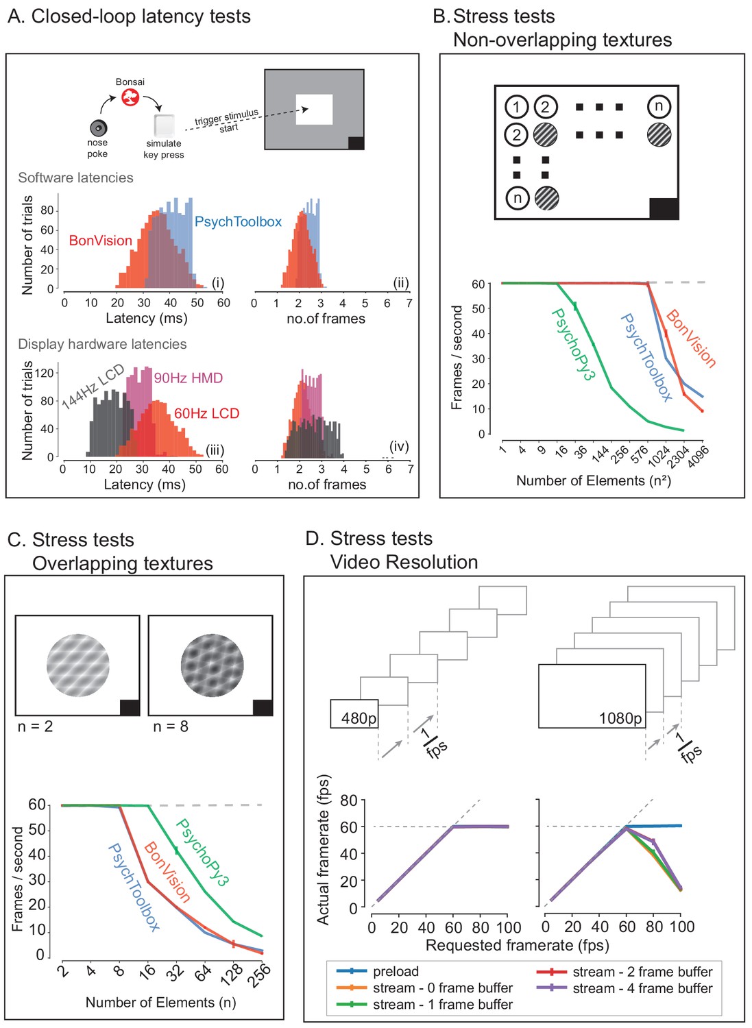
(A) Latency between sending a command (virtual key press) and updating the display (measured using a photodiode). (A.i and A.ii) Latency depended on the frame rate of the display, updating stimuli with a delay of one to three frames. (A.iii and A.iv). (B and C) Benchmarked performance of BonVision with respect to Psychtoolbox and PsychoPy. (B) When using non-overlapping textures BonVision and Psychtoolbox could present 576 independent textures without dropping frames, while PsychoPy could present 16. (C) When using overlapping textures PsychoPy could present 16 textures, while BonVision and Psychtoolbox could present eight textures without dropping frames. (D) Benchmarks for movie playback. BonVision is capable of displaying standard definition (480 p) and high definition (1080 p) movies at 60 frames/s on a laptop computer with a standard CPU and graphics card. We measured display rate when fully pre-loading the movie into memory (blue), or when streaming from disk (with no buffer: orange; 1-frame buffer: green; 2-frame buffer: red; 4-frame buffer: purple). When asked to display at rates higher than the monitor refresh rate (>60 frames/s), the 480 p video played at the maximum frame rate of 60fps in all conditions, while the 1080 p video reached the maximum rate when pre-loaded. Using a buffer slightly improved performance. A black square at the bottom right of the screen in A–C is the position of a flickering rectangle, which switches between black and white at every screen refresh. The luminance in this square is detected by a photodiode and used to measure the actual frame flip times.
Figure 4—figure supplement 1
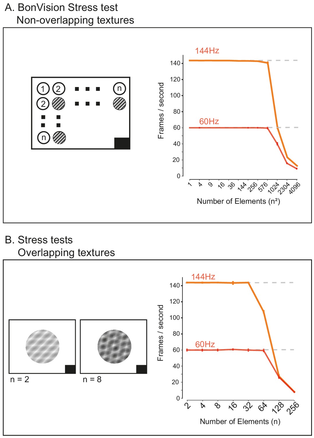
BonVision performance benchmarks at high frame rate.
(A) When using non-overlapping textures BonVision was able to render 576 independent textures without dropping frames at 60 Hz. At 144 Hz BonVision was able to 256 non-overlapping textures, with no dropped frames, and seldom dropped frames with 576 textures. BonVision was unable to render 1024 or more textures at the requested frame rate. (B) When using overlapping textures BonVision was able to render 64 independent textures without dropping frames at 60 Hz. At 144 Hz BonVision was able to render 32 textures, with no dropped frames. Note that these tests were performed on a computer with better hardware specification than that used in Figure 4, which led to improved performance on the benchmarks at 60 Hz. A black square at the bottom right of the screen in A and B is the position of a flickering rectangle, which switches between black and white at every screen refresh. The luminance in this square is detected by a photodiode and used to measure the actual frame flip times.
Figure 5 with 1 supplement
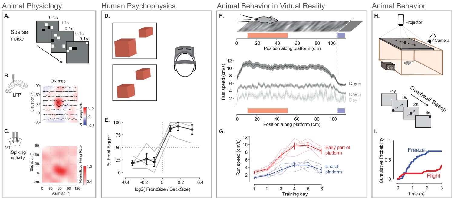
Illustration of BonVision across a range of vision research experiments.
(A) Sparse noise stimulus, generated with BonVision, is rendered onto a demi-spherical screen. (B and C) Receptive field maps from recordings of local field potential in the superior colliculus (B), and spiking activity in the primary visual cortex (C) of mouse. (D) Two cubes were presented at different depths in a virtual environment through a head-mounted display to human subjects. Subjects had to report which cube was larger: left or right. (E) Subjects predominantly reported the larger object correctly, with a slight bias to report that the object in front was bigger. (F) BonVision was used to generate a closed-loop virtual platform that a mouse could explore (top: schematic of platform). Mice naturally tended to run faster along the platform, and in later sessions developed a speed profile, where they slowed down as they approached the end of the platform (virtual cliff). (G) The speed of the animal at the start of the platform and at the end of the platform as a function training. (H) BonVision was used to present visual stimuli overhead while an animal was free to explore an environment (which included a refuge). The stimulus was a small dot (5° diameter) moving across the projected surface over several seconds. (I) The cumulative probability of Freeze and Flight behaviour across time in response to moving dot presented overhead.
Figure 5—figure supplement 1
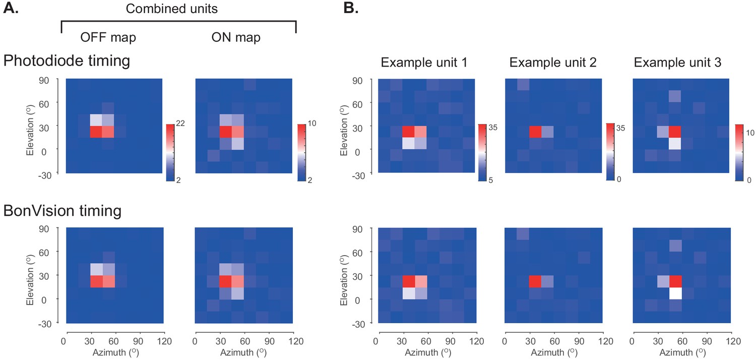
BonVision timing logs are sufficient to support receptive field mapping of spiking activity.
Top row in each case shows the receptive field identified using the timing information provided by a photodiode that monitored a small square on the stimulus display that was obscured from the animal. Bottom row in each case shows the receptive field identified by using the timing logged by BonVision during the stimulus presentation (a separate timing system was used to align the clocks between the computer hosting BonVision and the Open EPhys recording device). (A) Average OFF and ON receptive field maps for 33 simultaneously recorded units in a single recording session. (B) Individual OFF receptive field maps for three representative units in the same session.
Tables
Appendix 1—table 1
Features of visual display software.
| Features | BonVision | PsychToolbox | PsychoPy | ViRMEn | ratCAVE | FreemoVR | Unity |
|---|---|---|---|---|---|---|---|
| Free and Open-source (FOSS) | √√ | √# | √√ | √# | √ | √√ | √ |
| Rendering of 3D environments | √√ | √ | √ | √√ | √√ | √√ | √√ |
| Dynamic rendering based on observer viewpoint | √√ | √ | √√ | √√ | √ | ||
| GUI for designing 3D scenes | √√ | √√ | |||||
| Import 3rd party 3D scenes | √√ | √ | √ | √√ | |||
| Real-time interactive 3D scenes | √√ | √ | √√ | √√ | √√ | √√ | |
| Web-based deployment | √√ | √√ | |||||
| Interfacing with cameras, sensors and effectors | √√ | √√ | ~ | √√ | ~ | ~ | |
| Real-time hardware control | √√ | ~ | ~ | √ | √√ | √ | √ |
| Traditional visual stimuli | √√ | √√ | √√ | ||||
| Auto-calibration of display position and pose | √√ | ||||||
| Integration with deep learning pose estimation | √√ |
-
√√ easy and well-supported.
√ possible, not well-supported.
-
~ difficult to implement.
# based on MATLAB (requires a license).
Additional files
Download links
A two-part list of links to download the article, or parts of the article, in various formats.
Downloads (link to download the article as PDF)
Open citations (links to open the citations from this article in various online reference manager services)
Cite this article (links to download the citations from this article in formats compatible with various reference manager tools)
Creating and controlling visual environments using BonVision
eLife 10:e65541.
https://doi.org/10.7554/eLife.65541


