Distinct higher-order representations of natural sounds in human and ferret auditory cortex
- Laboratoire des Systèmes Perceptifs, Département d’Études Cognitives, École Normale Supérieure PSL Research University, CNRS, France
- University College London, United Kingdom
- Physics for Medicine Paris, Inserm, ESPCI Paris, PSL Research University, CNRS, France
- Institute for Systems Research, Department of Electrical and Computer Engineering, University of Maryland, United States
- HHMI Postdoctoral Fellow of the Life Sciences Research Foundation, United States
- Zuckerman Mind Brain Behavior Institute, Columbia University, United States
Figures
Figure 1 with 2 supplements

Schematic of stimuli and imaging protocol.
(A) Cochleagrams for two example natural sounds (left column) and corresponding synthetic sounds (right four columns) that were matched to the natural sounds along a set of acoustic statistics of increasing complexity. Statistics were measured by filtering a cochleagram with filters tuned to temporal, spectral, or joint spectrotemporal modulations. (B) Schematic of the imaging procedure. A three-dimensional volume, covering all of ferret auditory cortex, was acquired through successive coronal slices. Auditory cortical regions (colored regions) were mapped with anatomical and functional markers (Radtke-Schuller, 2018). The rightmost image shows a single ultrasound image with overlaid region boundaries. Auditory regions: dPEG: dorsal posterior ectosylvian gyrus; AEG: anterior ectosylvian gyrus; VP: ventral posterior auditory field; ADF: anterior dorsal field; AAF: anterior auditory field. Non-auditory regions: hpc: hippocampus; SSG: suprasylvian gyrus; LG: lateral gyrus. Anatomical markers: pss: posterior sylvian sulcus; sss: superior sylvian sulcus. (C) Response timecourse of a single voxel to all natural sounds, before (left) and after (right) denoising. Each line reflects a different sound, and its color indicates its membership in one of 10 different categories. English and non-English speech are separated out because all of the human subjects tested in our prior study were native English speakers, and so the distinction is meaningful in humans. The gray region shows the time window when sound was present. We summarized the response of each voxel by measuring its average response to each sound between 3 and 11 s post-stimulus onset. The location of this voxel corresponds to the highlighted voxel in panel B. (D) We measured the correlation across sounds between pairs of voxels as a function or their distance using two independent measurements of the response (odd vs. even repetitions). Results are plotted separately for ferret fUS data (left) and human fMRI data (right). The 0 mm datapoint provides a measure of test–retest reliability and the fall-off with distance provides a measure of spatial precision. Results are shown before and after component denoising. Note that in our prior fMRI study we did not use component denoising because the voxels were sufficiently reliable; we used component-denoised human data here to make the human and ferret analyses more similar (findings did not depend on this choice: see Figure 1—figure supplement 2). The distance needed for the correlation to decay by 75% is shown above each plot (). The human data were smoothed using a 5 MM FWHM kernel, the same amount used in our prior study, but fMRI responses were still coarser when using unsmoothed data ( = 6.5 mm; findings did not depend on the presence/absence of smoothing). Thin lines show data from individual human (N = 8) and ferret (N = 2) subjects, and thick lines show the average across subjects.
Figure 1—figure supplement 1
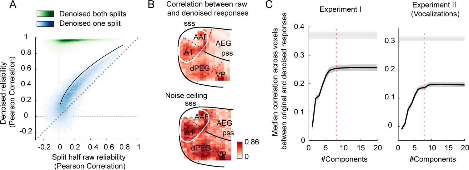
The effect of enhancing reliable signal using a procedure similar to ‘denoising source separation (DSS)’ (see ‘Denoising part II’ in Materials and methods) (de Cheveigné and Parra, 2014).
(A) Voxel responses were denoised by projecting their timecourse onto components that were reliably present across repetitions and slices. This figure plots the test–retest correlation across independent splits of data before (x-axis) and after (y-axis) denoising (data from experiment I). Each dot corresponds to a single voxel. We denoised either one split of data (blue dots) or both splits of data (green dots). Denoising one split provides a fairer test of whether the denoising procedure enhances SNR. Denoising both splits shows the overall effect on response reliability. The theoretical upper bound for denoising one split of data is shown by the black line. The denoising procedure substantially increased data reliability, with the one-split correlations hugging the upper bound. This plot shows results from an eight-component model. (B) This figure plots split-half correlations for denoised data (one split) as a map (upper panel), along with a map showing the upper bound (lower panel). Denoised correlations were close to their upper bound throughout auditory cortex. (C) This figure plots the median denoised correlation across voxels (one split) as a function of the number of components used in the denoising procedure. Gray line plots the upper bound. Shaded areas indicate the 95% confidence interval, computed via bootstrapping across the sound set. Results are shown for both experiments I (left) and II (right). Predictions were near their maximum using approximately eight components in both experiments (the eight-component mark is shown by the vertical dashed line).
Figure 1—figure supplement 2
Effect of component denoising on human fMRI results.
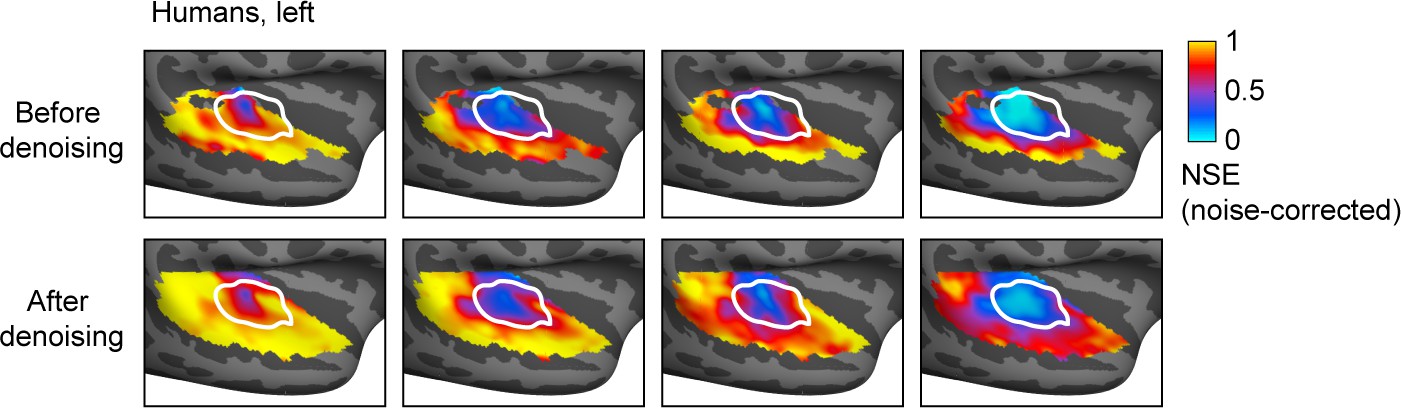
This figure plots normalized squared error (NSE) maps comparing natural and synthetic sounds in humans both before (top) and after denoising (bottom) by projecting onto the six reliable components identified in our prior work (Norman-Haignere et al., 2015). We used component-denoised data for all species comparisons to make the analyses more similar, but results were similar without denoising. The bottom panel is the same as that shown in Figure 2E and is reproduced here for ease of comparison. Results are based on 12 human subjects.
Figure 2 with 3 supplements
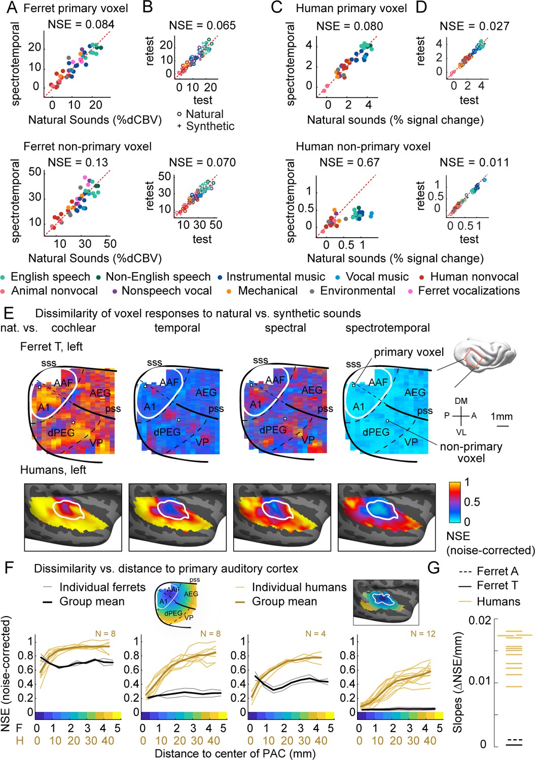
Dissimilarity of responses to natural vs. synthetic sounds in ferrets and humans.
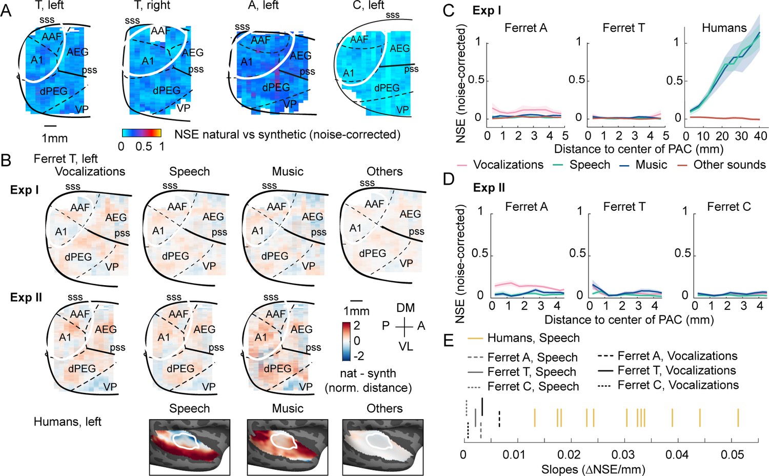
(A) Response of two example fUS voxels to natural and corresponding synthetic sounds with matched spectrotemporal modulation statistics. Each dot shows the time-averaged response to a single pair of natural/synthetic sounds (after denoising), with colors indicating the sound category. The example voxels come from primary (top, A1) and non-primary (bottom, dPEG) regions of the ferret auditory cortex (locations shown in panel E). The normalized squared error (NSE) quantifies the dissimilarity of responses. (B) Test–retest response of the example voxels across all natural (o) and synthetic (+) sounds (odd vs. even repetitions). The responses were highly reliable due to the denoising procedure. (C, D) Same as panels (A, B), but showing two example voxels from human primary/non-primary auditory cortex. (E) Maps plotting the dissimilarity of responses to natural vs. synthetic sounds from one ferret hemisphere (top row) and from humans (bottom row). Each column shows results for a different set of synthetic sounds. The synthetic sounds were constrained by statistics of increasing complexity (from left to right): just cochlear statistics, cochlear + temporal modulation statistics, cochlear + spectral modulation statistics, and cochlear + spectrotemporal modulation statistics. Dissimilarity was quantified using the NSE, corrected for noise using the test–retest reliability of the voxel responses. Ferret maps show a ‘surface’ view from above of the sylvian gyri, similar to the map in humans. Surface views were computed by averaging activity perpendicular to the cortical surface. The border between primary and non-primary auditory cortex is shown with a white line in both species and was defined using tonotopic gradients. Areal boundaries in the ferret are also shown (dashed thin lines). This panel shows results from one hemisphere of one animal (ferret T, left hemisphere), but results were similar in other animals/hemispheres (Figure 2—figure supplement 2). The human map is a group map averaged across 12 subjects, but results were similar in individual subjects (Norman-Haignere et al., 2018). (F) Voxels were binned based on their distance to primary auditory cortex (defined tonotopically). This figure plots the median NSE value in each bin. Each thin line corresponds to a single ferret (gray) or a single human subject (gold). Thick lines show the average across all subjects. The ferret and human data were rescaled so that they could be plotted on the same figure, using a scaling factor of 10, which roughly corresponds to the difference in the radius of primary auditory cortex between ferrets and humans. The corresponding unit is plotted on the x-axis below. The number of human subjects varied by condition (see Materials and methods for details) and is indicated on each plot. (G) The slope of NSE vs. distance-to-primary auditory cortex (PAC) curve (F) from individual ferret and human subjects using responses to the spectrotemporally matched synthetic sounds. We used absolute distances to quantify the slope, which is conservative with respect to the hypothesis since correcting for brain size would differentially increase the ferret slopes.
Figure 2—figure supplement 1

Responses to natural and synthetic sounds in standard anatomical regions of interest (ROIs).
Format is analogous to Figure 2A and B. (A) Cartoon showing the location of three ROIs spanning primary (MEG) and non-primary (AEG, PEG) ferret auditory cortex. (B) Response to natural and spectrotemporally matched synthetic sounds averaged across all voxels in each ROI. Each circle corresponds to a single pair of natural/synthetic sounds, with colors indicating the sound category. The normalized squared error (NSE) between natural and synthetic sounds is shown above each plot. (C) Test–retest response of the ROI across all natural (o) and synthetic (+) sounds (odd vs. even repetitions). The test–retest NSE provides a noise floor for the natural vs. synthetic NSE.
Figure 2—figure supplement 2
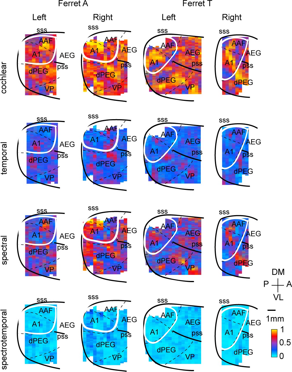
Dissimilarity maps for all hemispheres and animals.
Same format as Figure 2E.
Figure 2—figure supplement 3

Uncorrected normalized squared error (NSE) values.
This figure plots the uncorrected NSE between natural and synthetic sounds as a function of distance to primary auditory cortex (PAC) for humans (A) and ferrets (B). The test–retest NSE value, which provides a noise floor for the natural vs. synthetic NSE, is plotted below each set of curves using dashed lines. Each thin line corresponds to a single ferret (gray) or a single human subject (gold). Thick lines show the average across all subjects. Format is the same as Figure 2F.
Figure 3 with 5 supplements
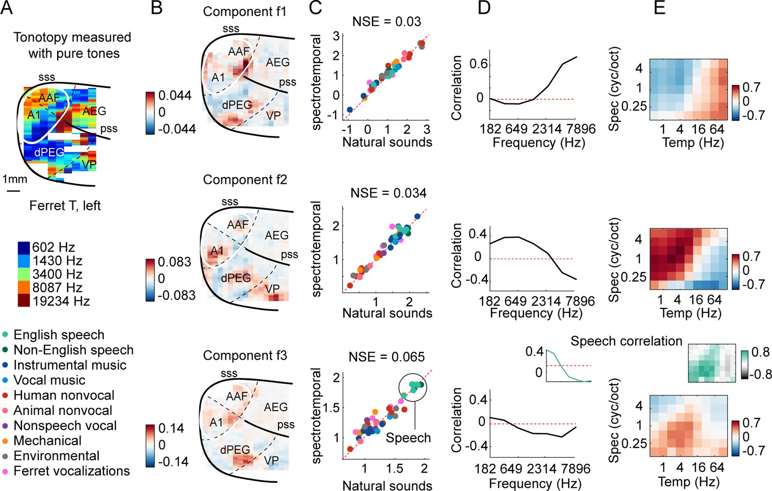
Organization of frequency and modulation tuning in ferret auditory cortex, as revealed by component analysis.
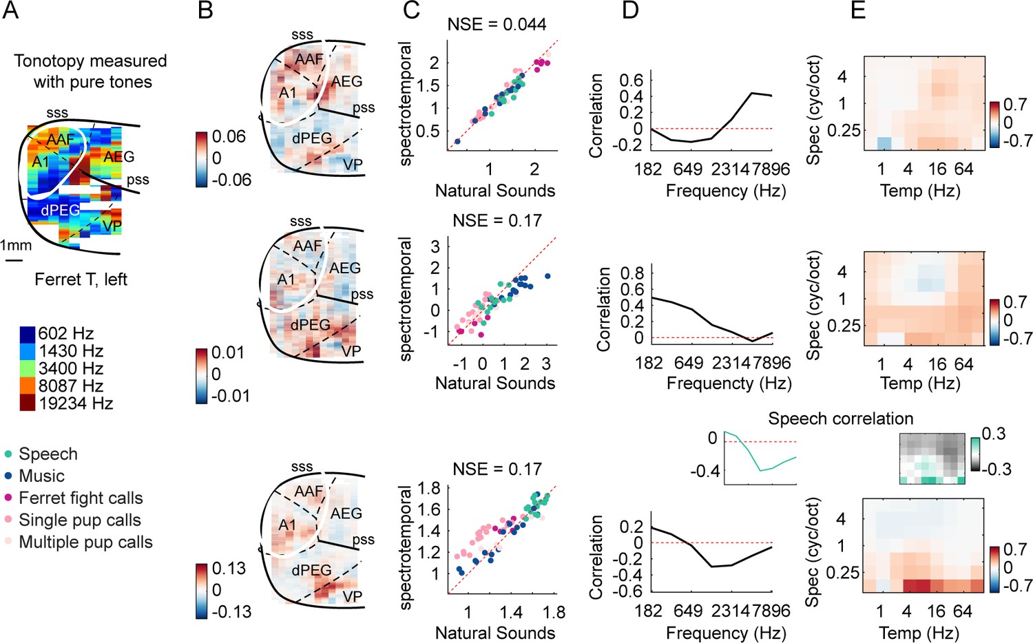
(A) For reference with the weight maps in panel (B), a tonotopic map is shown, measured using pure tones. The map is from one hemisphere of one animal (ferret T, left). (B) Voxel weight maps from three components, inferred using responses to natural and synthetic sounds (see Figure 3—figure supplement 1 for all eight components and Figure 3—figure supplement 2 for all hemispheres). The maps for components f1 and f2 closely mirrored the high- and low-frequency tonotopic gradients, respectively. (C) Component response to natural and spectrotemporally matched synthetic sounds, colored based on category labels (labels shown at the bottom left of the figure). Component f3 responded preferentially to speech sounds. (D) Correlation of component responses with energy at different audio frequencies, measured from a cochleagram. Inset for f3 shows the correlation pattern that would be expected from a response that was perfectly speech selective (i.e., 1 for speech, 0 for all other sounds). (E) Correlations with modulation energy at different temporal and spectral rates. Inset shows the correlation pattern that would be expected for a speech-selective response. Results suggest that f3 responds to particular frequency and modulation statistics that happen to differ between speech and other sounds.
Figure 3—figure supplement 1
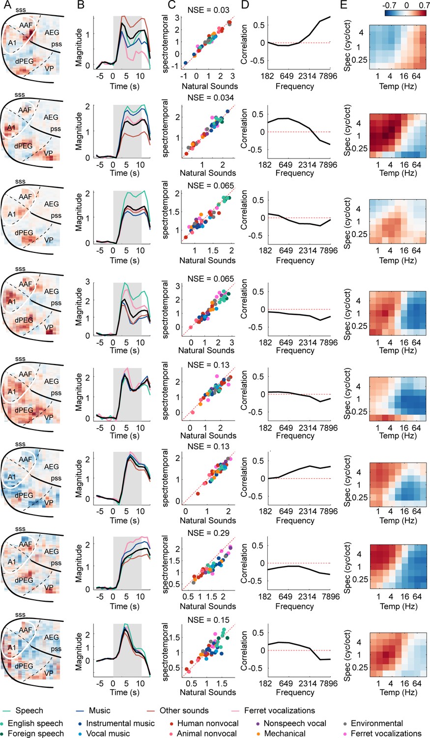
Results from all eight ferret components.
(A) Voxel weight map for each component. (B) The temporal response of each component. Black line shows the average timecourse across all natural sounds. Colored lines correspond to major categories (see Supplementary file 1): speech (green), music (blue), vocalizations (pink), and other sounds (brown). Note that the temporal shape varies across components, but is very similar across sounds/categories within a component, which is why we summarized component responses by their time-averaged response to each sound. (C) Time-averaged component responses to natural and spectrotemporally matched synthetic sounds, colored based on category labels. (D) Correlation of component responses with energy at different audio frequencies, measured from a cochleagram. (E) Correlations with modulation energy at different temporal and spectral rates.
Figure 3—figure supplement 2
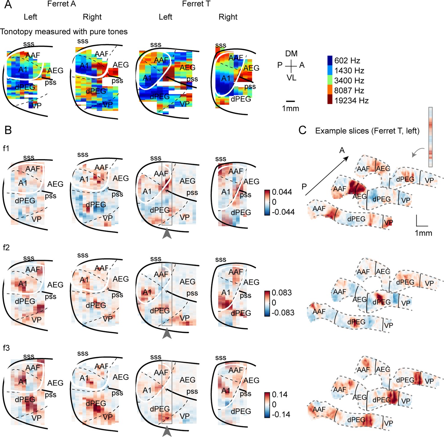
Component weight maps from all hemispheres and ferrets.
(A) For reference with the weight maps in panel (B), tonotopic maps measured using pure tones are shown for all hemispheres. (B) Voxel weight maps from the three components shown in Figure 3 for all hemispheres of all ferrets tested. (C) Voxel weights for three example coronal slices from ferret T, left hemisphere. Gray outlines in panel (B) indicate their location in the ‘surface’ view. Each slice corresponds to one vertical strip from the maps in panel (B). The same slices are shown for all three components.
Figure 3—figure supplement 3
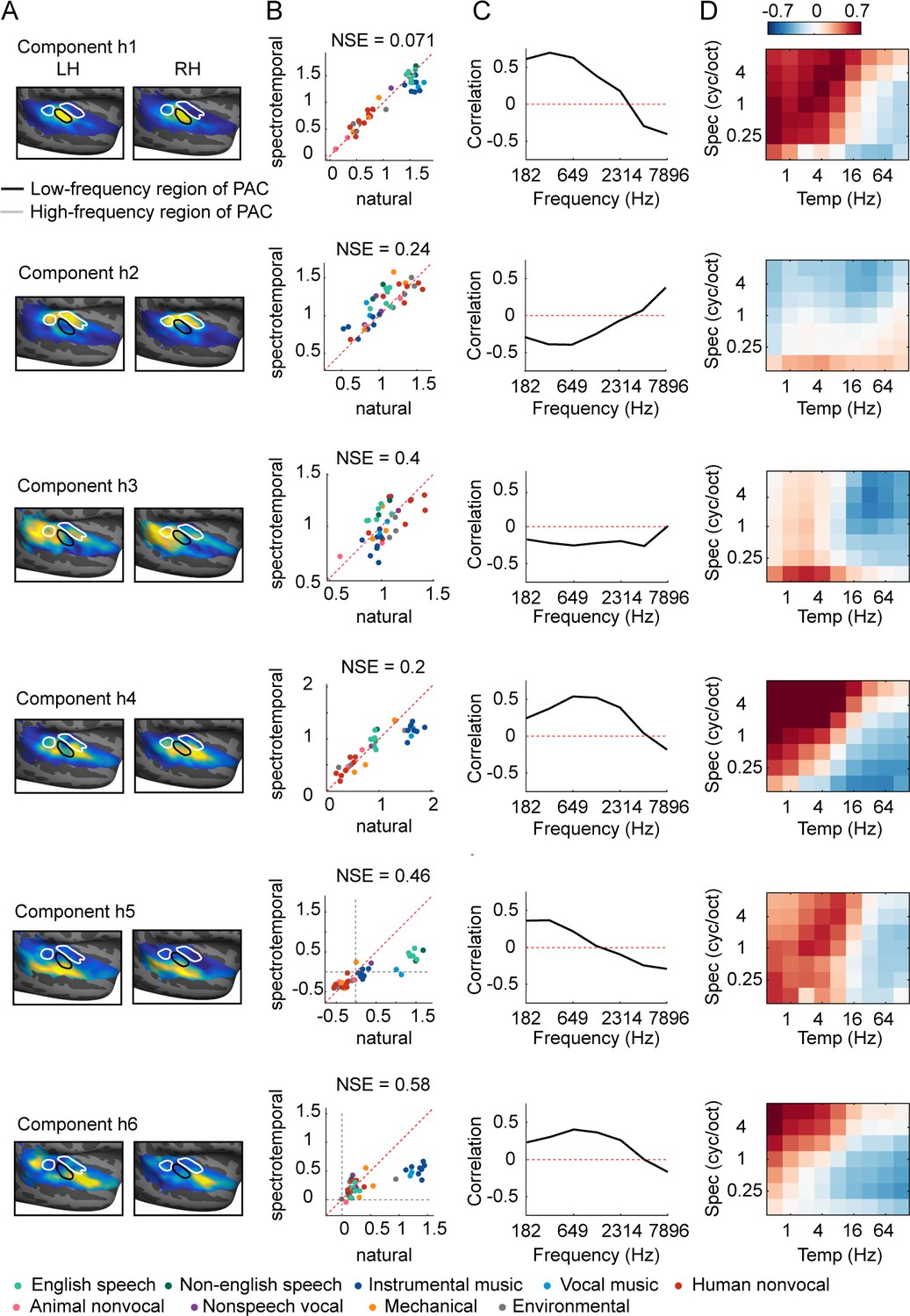
Human components.
This figure shows the anatomy and response properties of the six human components inferred in prior work (Norman-Haignere et al., 2015; Norman-Haignere et al., 2018). (A) Voxel weight map for each component, averaged across subjects. (B) Component responses to natural and spectrotemporally matched synthetic sounds, colored based on category labels. (C) Correlation of component responses with energy at different audio frequencies, measured from a cochleagram. (D) Correlations with modulation energy at different temporal and spectral rates.
Figure 3—figure supplement 4

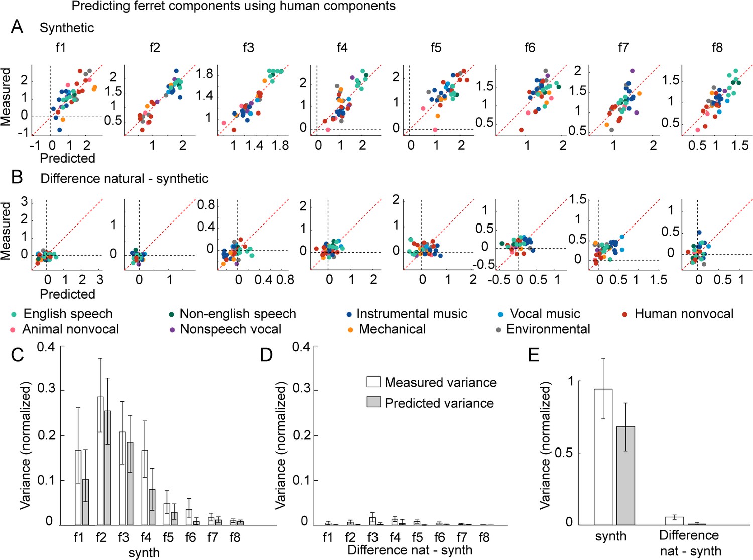
Predicting human component responses from ferret components.
This figure plots the results of trying to predict the six human components inferred from our prior work (Norman-Haignere et al., 2015; Norman-Haignere et al., 2018) from the eight ferret components inferred here (see Figure 3—figure supplement 5 for the reverse). (A) For reference, the response of the six human components to natural and spectrotemporally matched synthetic sounds is re-plotted here. Components h1–h4 produced similar responses to natural and synthetic sounds and had weights that clustered in and around primary auditory cortex (Figure 3—figure supplement 3). Components h5 and h6 responded selectively to natural speech and natural music, respectively, and had weights that clustered in non-primary regions. (B) This panel plots the measured response of each human component to just the spectrotemporally matched synthetic sounds, along with the predicted response from ferrets. (C) This panel plots the difference between responses to natural and spectrotemporally matched synthetic sounds along with the predicted difference from the ferret components. (D) This panel plots the total response variance (white bars) of each human component to synthetic sounds (left) and to the difference between natural and synthetic sounds (right) along with the fraction of that total response variance predictable from ferrets (gray bars) (all variance measures are noise-corrected). Error bars show the 95% confidence interval, computed via bootstrapping across the sound set. (E) Same as (D), but averaged across components.
Figure 3—figure supplement 5
Predicting ferret component responses from human components.
(A) This panel plots the measured response of each ferret component to just the spectrotemporally matched synthetic sounds, along with the predicted response from humans. (B) This panel plots the difference between responses to natural and spectrotemporally matched synthetic sounds along with the predicted difference from the human components. (C-D) This panel plots the total response variance (white bars) of each ferret component to synthetic sounds (C) and to the difference between natural and synthetic sounds (D) along with the fraction of that total response variance predictable from humans (gray bars) (all variance measures are noise-corrected). Error bars show the 95% confidence interval, computed via bootstrapping across the sound set. (E) Same as (C-D), but averaged across components.
Figure 4 with 3 supplements
Testing the importance of ecological relevance.
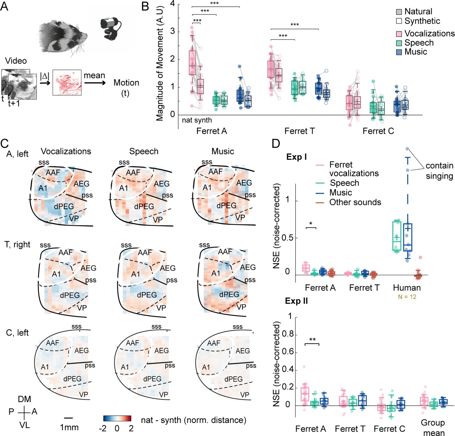
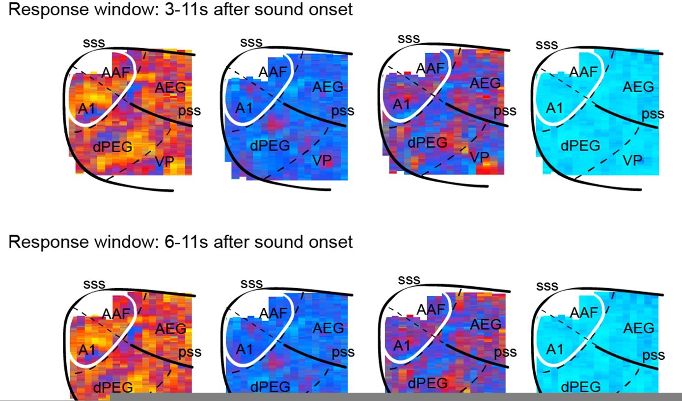
Experiment II measured responses to a larger number of ferret vocalizations (30 compared with 4 in experiment I), as well as speech (14) and music (16) sounds. (A) Map showing the dissimilarity between natural and spectrotemporally matched synthetic sounds from experiment II for each recorded hemisphere, measured using the noise-corrected normalized squared error (NSE). NSE values were low across auditory cortex, replicating experiment I. (B) Maps showing the average difference between responses to natural and synthetic sounds for vocalizations, speech, music, and others sounds, normalized for each voxel by the standard deviation across all sounds. Results are shown for ferret T, left hemisphere for both experiments I and II (see Figure 4—figure supplement 1C for all hemispheres). For comparison, the same difference maps are shown for the human subjects, who were only tested in experiment I. (C) NSE for different sound categories, plotted as a function of distance to primary auditory cortex (binned as in Figure 2F). Shaded area represents 1 standard error of the mean across sounds within each category (Figure 4—figure supplement 1D plots NSEs for individual sounds). (D) Same as panel (C) but showing results from experiment II. (E) The slope of NSE vs. distance-to-primary auditory cortex (PAC) curves for individual ferrets and human subjects. Ferret slopes were measured separately for ferret vocalizations (black lines) and speech (gray lines) (animal indicated by line style). For comparison, human slopes are plotted for speech (each yellow line corresponds to a different human subject).
Figure 4—figure supplement 1
Results of experiment II from other hemispheres.
(A) The animal’s spontaneous movements were monitored with a video recording of the animal’s face. Motion was measured as the mean absolute deviation between adjacent video frames, averaged across pixels. (B) Average evoked movement amplitude for natural (shaded) and synthetic (unshaded) sounds broken down by category. Each dot represents one sound. Significant differences between natural and synthetic sounds, and between categories of natural sounds are plotted (Wilcoxon signed-rank test, *p<0.05; **p<0.01; ***p<0.001). Evoked movement amplitude was normalized by the standard deviation across sounds for each recording session prior to averaging across sound category (necessary because absolute pixel deviations cannot be meaningfully compared across sessions). Movement amplitude is shown for each animal separately. (C) Same format as Figure 4B but showing results from additional hemispheres/animals. (D) This panel shows the distribution of normalized squared error (NSE) values for all pairs of natural and synthetic sounds (median across all voxels; averaged across subjects for humans), grouped by category. Dots show individual sound pairs and boxplots show the median, central 50%, and central 92% (whiskers) of the distribution. Humans were only tested in experiment I. Note that the two outliers for the human music plot are sound clips that contain singing, and thus are a mixture of both speech and music, which likely explains the particularly divergent responses.
Figure 4—figure supplement 2
Components from experiment II.
The components derived from experiment II were similar to those from experiment I, shown in Figure 3. This figure plots similar low-frequency, high-frequency, and speech-preferring components from experiment II. Figure 3 (A) For reference with the weight maps in panel (B), a tonotopic map is shown, measured using pure tones. The map is from one hemisphere of one animal (ferret T, left). (B) Voxel weight maps. (C) Component response to natural and spectrotemporally matched synthetic sounds, colored based on category labels (labels shown at the bottom left of the figure). (D) Correlation of component responses with energy at different audio frequencies, measured from a cochleagram. Inset for f3 shows the correlation pattern that would be expected from a response that was perfectly speech selective (i.e., 1 for speech, 0 for all other sounds). (E) Correlations with modulation energy at different temporal and spectral rates. Inset shows the correlation pattern that would be expected for a speech-selective response.
Figure 4—figure supplement 3
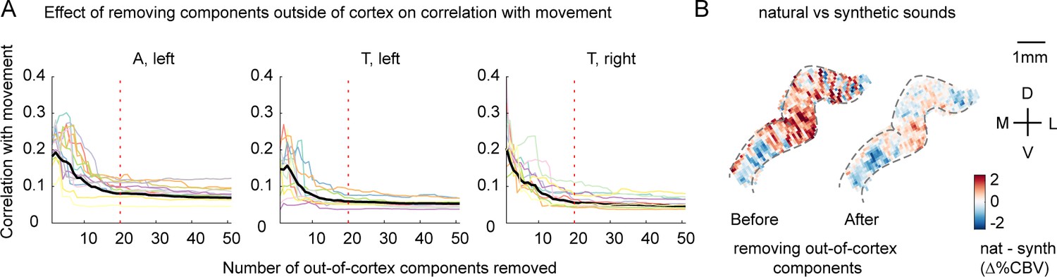
The effect of removing outside-of-cortex components on motion correlations.
Voxel responses were denoised by removing components from outside of cortex, which are likely to reflect artifacts like motion (see ‘Denoising part I’ in Materials and methods). (A) Effect of removing components from outside of cortex on correlations with movement. We measured the correlation of each voxel’s response with movement, measured from a video recording of the animal’s face (absolute deviation between adjacent frames). Each line shows the average absolute correlation across voxels for a single recording session/slice. Correlation values are plotted as a function of the number of removed components. Motion correlations were substantially reduced by removing the top 20 components (vertical dotted line). (B) The average difference between responses to natural vs. synthetic sounds for an example slice (ferret A) before and after removing the top 20 out-of-cortex components. Motion induces a stereotyped ‘striping’ pattern due to its effect on blood vessels, which is evident in the map computed from raw data, likely because this ferret moved substantially more during natural vs. synthetic sounds (in particular for ferret vocalizations; Figure 4—figure supplement 1). The striping pattern is unlikely to reflect genuine neural activity and is largely removed by the denoising procedure.
Appendix 1—figure 1
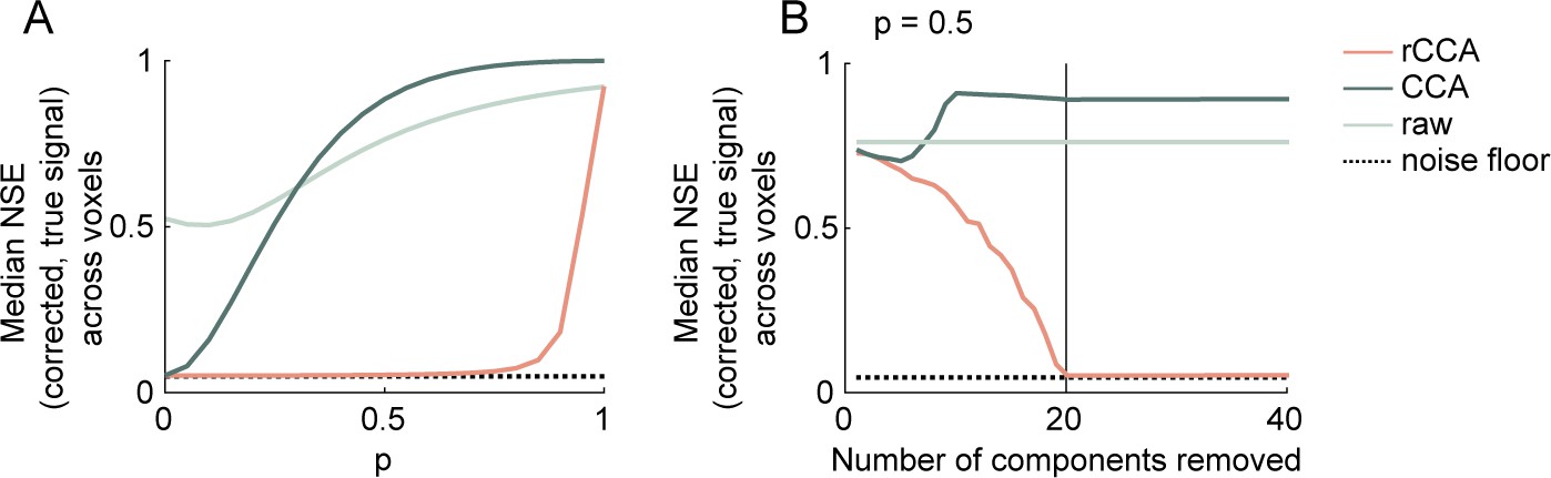
Simulation results.
(A) Median normalized squared error (NSE) across simulated voxels between the true and estimated sound-driven responses (), computed using raw/undenoised data (light green line), standard canonical correlation analysis (CCA) (dark green line), and recentered CCA (red line). Results are shown as a function of the strength of the dependence () between sound-driven and artifactual timecourses. The minimum possible NSE (noise floor) given the level of voxel-specific noise is also shown. (B) Same as panel (A), but showing results as a function of the number of components removed for a fixed value of (set to 0.5).
Author response image 1
Additional files
-
Supplementary file 1
List of sounds used in both experiments.
Names of sounds used in experiments I and II, grouped by category at both fine and coarse scales.
- https://cdn.elifesciences.org/articles/65566/elife-65566-supp1-v1.ai
-
Transparent reporting form
- https://cdn.elifesciences.org/articles/65566/elife-65566-transrepform1-v1.docx
Download links
A two-part list of links to download the article, or parts of the article, in various formats.
Downloads (link to download the article as PDF)
Open citations (links to open the citations from this article in various online reference manager services)
Cite this article (links to download the citations from this article in formats compatible with various reference manager tools)
Distinct higher-order representations of natural sounds in human and ferret auditory cortex
eLife 10:e65566.
https://doi.org/10.7554/eLife.65566


