A quadratic model captures the human V1 response to variations in chromatic direction and contrast
- Department of Psychology, University of Pennsylvania, United States
- Department of Neurology, University of Pennsylvania, United States
Figures
Figure 1
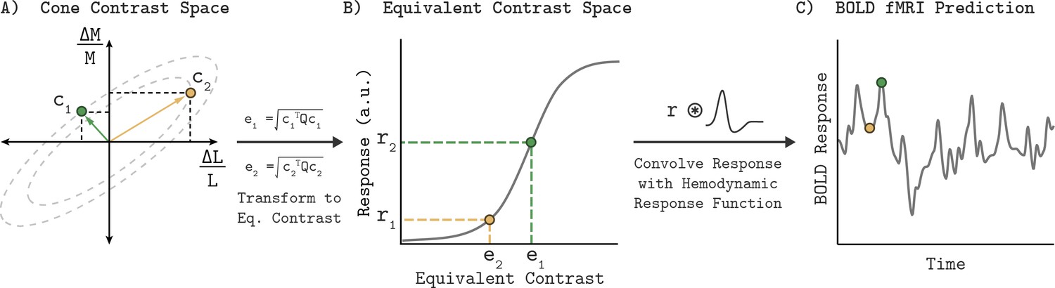
Quadratic color model.
(A) The LM contrast plane representing two example stimuli (c1 and c2) as the green and yellow vectors. The vector length and direction specify the contrast and chromatic direction of the positive arm of the symmetric modulation (see Visual Stimuli in Materials and methods). Using the parameters of an elliptical isoresponse contour (panel A, dashed gray ellipses), fit per subject, we can construct a 2x2 matrix Q that allows us to compute the equivalent contrast of any stimulus in the LM contrast plane (panel B; e1 and e2; see Appendix 1). (B) Transformation of equivalent contrast to neuronal response. The equivalent contrasts of the two example stimuli from panel A are plotted against their associated neuronal response. A single Naka-Rushton function describes the relationship between equivalent contrast and the underlying neuronal response. (C) To predict the BOLD fMRI response, we convolve the neuronal response output of the Naka-Rushton function with a subject-specific hemodynamic response function. Note that the BOLD fMRI response prediction for the green point is greater than the prediction for the yellow point, even though the yellow point has greater cone contrast. This is because of where the stimuli lie relative to the isoresponse contours. The difference in chromatic direction results in the green point producing a greater equivalent contrast, resulting in the larger BOLD response.
Figure 2 with 2 supplements
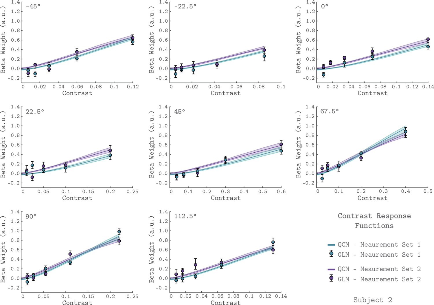
V1 contrast response functions for the eight measured chromatic directions from Subject 2.
Each panel plots the contrast response function of V1, aggregated over 0° to 20° eccentricity, for a single chromatic direction. The x-axis is contrast, the y-axis is the BOLD response (taken as the GLM beta weight for each stimulus). The chromatic direction of each stimulus is indicated in the upper left of each panel. The curves represent the QCM prediction of the contrast response function. Error bars indicate 68% confidence intervals obtained by bootstrap resampling. Measurement Sets 1 and 2 are shown in green and purple. The x-axis range differs across panels as the maximum contrast used varies with chromatic direction. All data shown have had the baseline estimated from the background condition subtracted such that we obtain a 0 beta weight at 0 contrast.
Figure 2—figure supplement 1
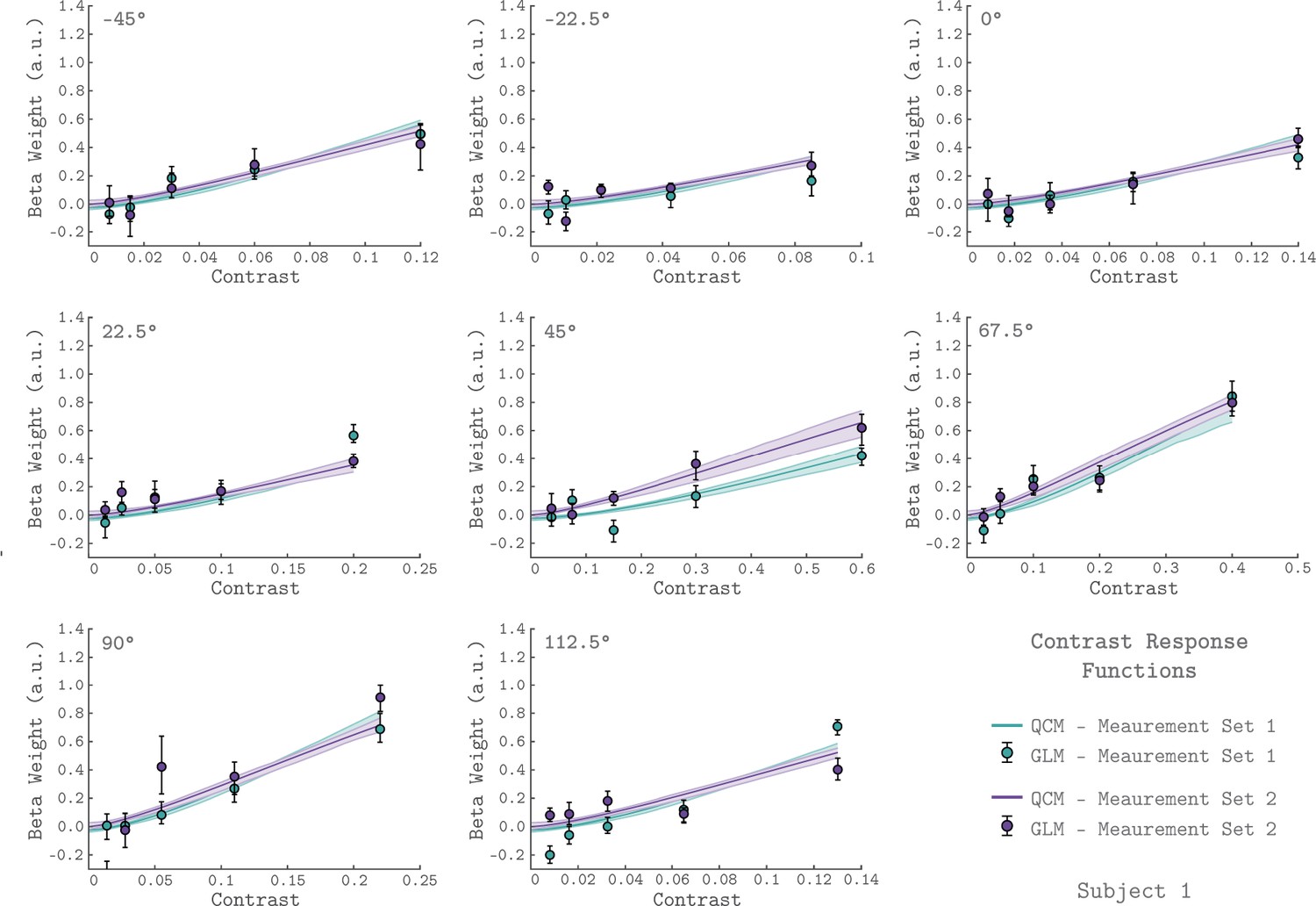
V1 contrast response functions for the eight measured chromatic directions from Subject 1.
The format of the figure is the same as Figure 2 in the main text. The x-axis is contrast; the y-axis is the beta weight of the GLM. The chromatic direction of each stimulus is indicated in the upper left of each panel. The curves in each panel represent the contrast response function obtained using the QCM. The error bars indicate 68% confidence intervals obtained using bootstrapping. Measurement sets 1 and 2 are shown in green and purple. The x-axis range differs across panels as the maximum contrast used varies with color direction.
Figure 2—figure supplement 2
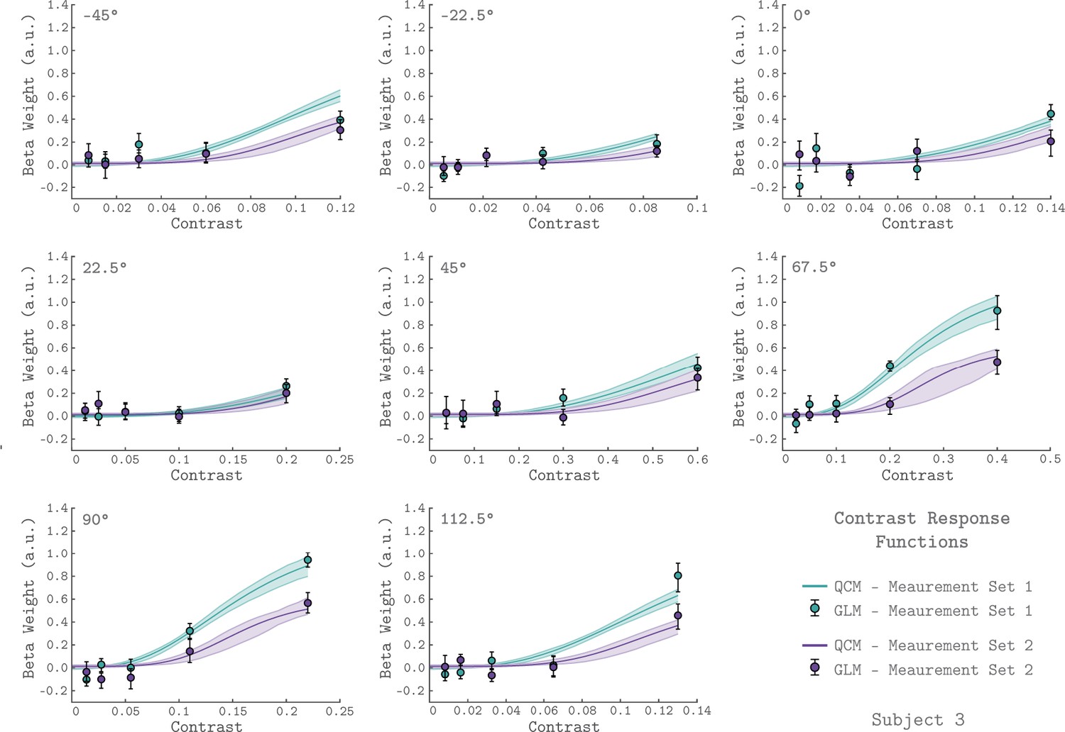
V1 contrast response functions for the eight measured chromatic directions from Subject 3.
The format of the figure is the same as Figure 2 in the main text and Figure 2—figure supplement 1.
Figure 3 with 3 supplements
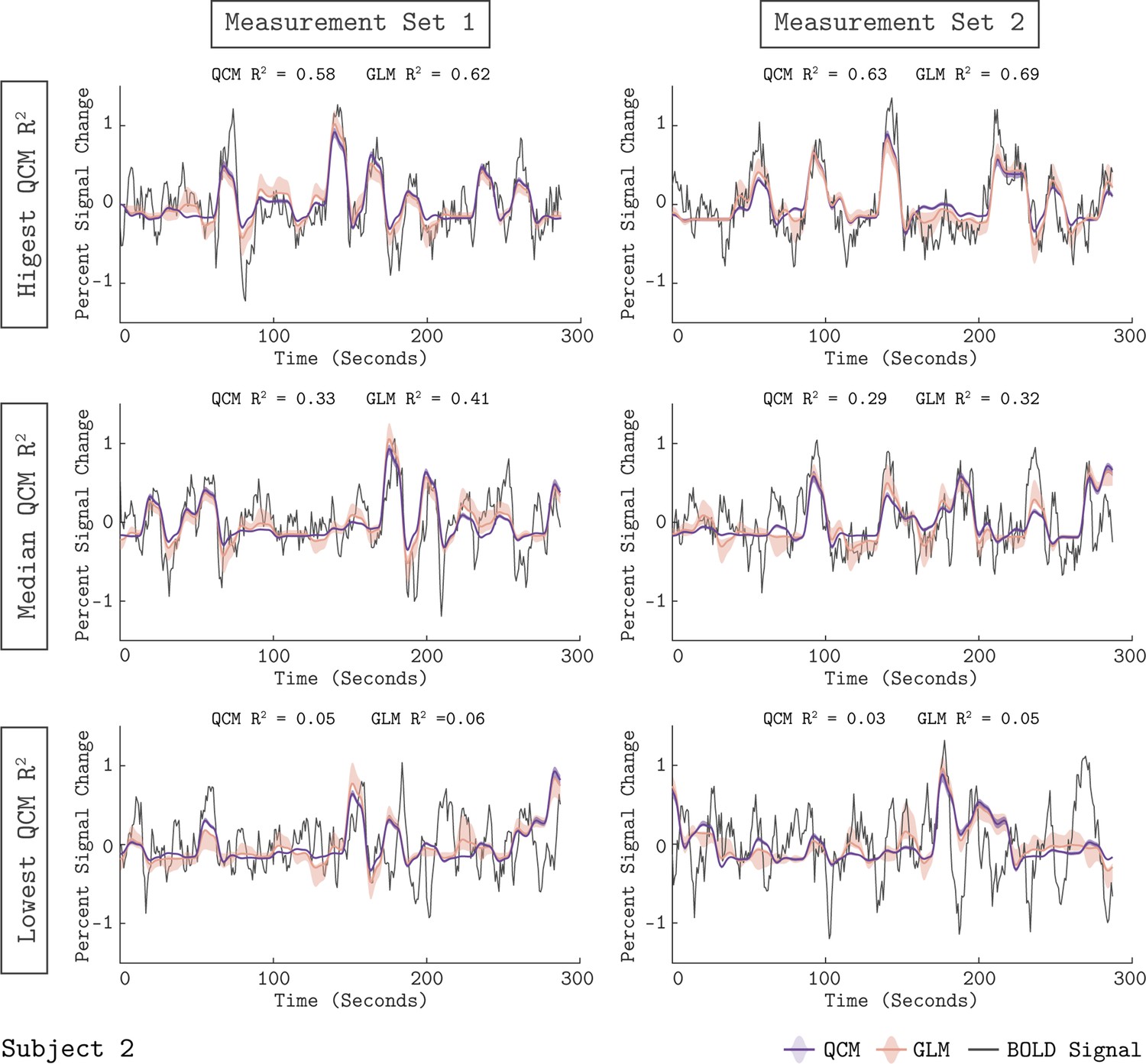
Model fits to the V1 BOLD time course.
The measured BOLD time course (thin gray line) is shown along with the model fits from the QCM (thick purple line) and GLM (thin orange line) for six runs from Subject 2. Individual runs consisted of only half the total number of chromatic directions. The left column shows data and fits from Measurement Set one and the right column for Measurement Set 2. The three runs presented for each measurement set were chosen to correspond to the highest, median, and lowest QCM R2 values within the respective measurement set; the ranking of the GLM R2 values across runs was similar. The R2 values for the QCM and the GLM are displayed at the top of each panel. The shaded error regions represent the 68% confidence intervals for the GLM obtained using bootstrapping.
Figure 3—figure supplement 1
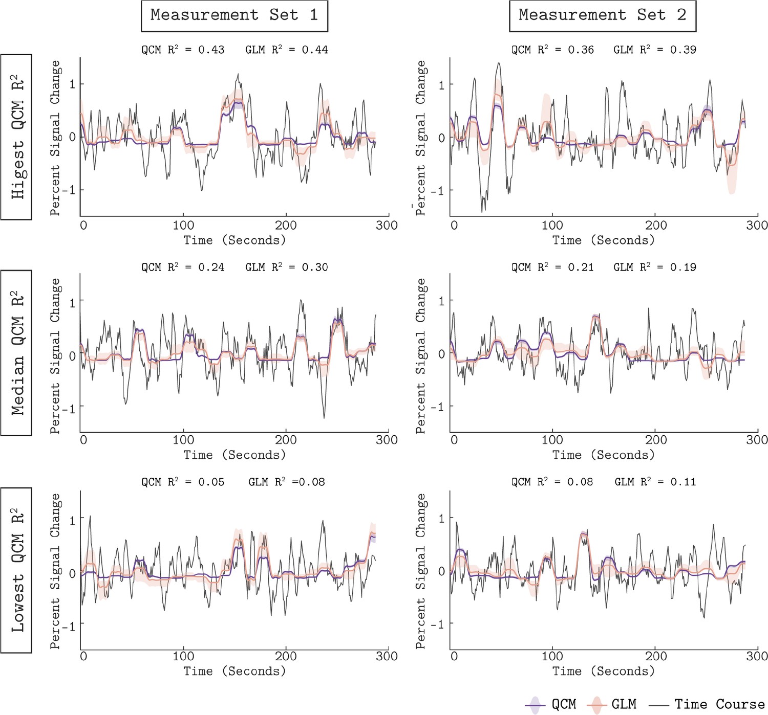
Model fits to the V1 BOLD time course from Subject 1.
The format of the Figure is the same as Figure 3 in the main text. The measured BOLD time course (black line) is shown along with the model outputs from the QCM (thick purple line) and GLM (thin orange line) for six acquisitions. The left column shows data and fits from Measurement Set 1 and the right column for Measurement Set 2. The three acquisitions presented for each measurement set were chosen to correspond to the highest, median, and lowest QCM R2 values within the respective measurement set. The R2 values for the QCM and the GLM are displayed at the top of each panel. The shaded regions represent the 68% confidence intervals obtained via the bootstrap analysis.
Figure 3—figure supplement 2
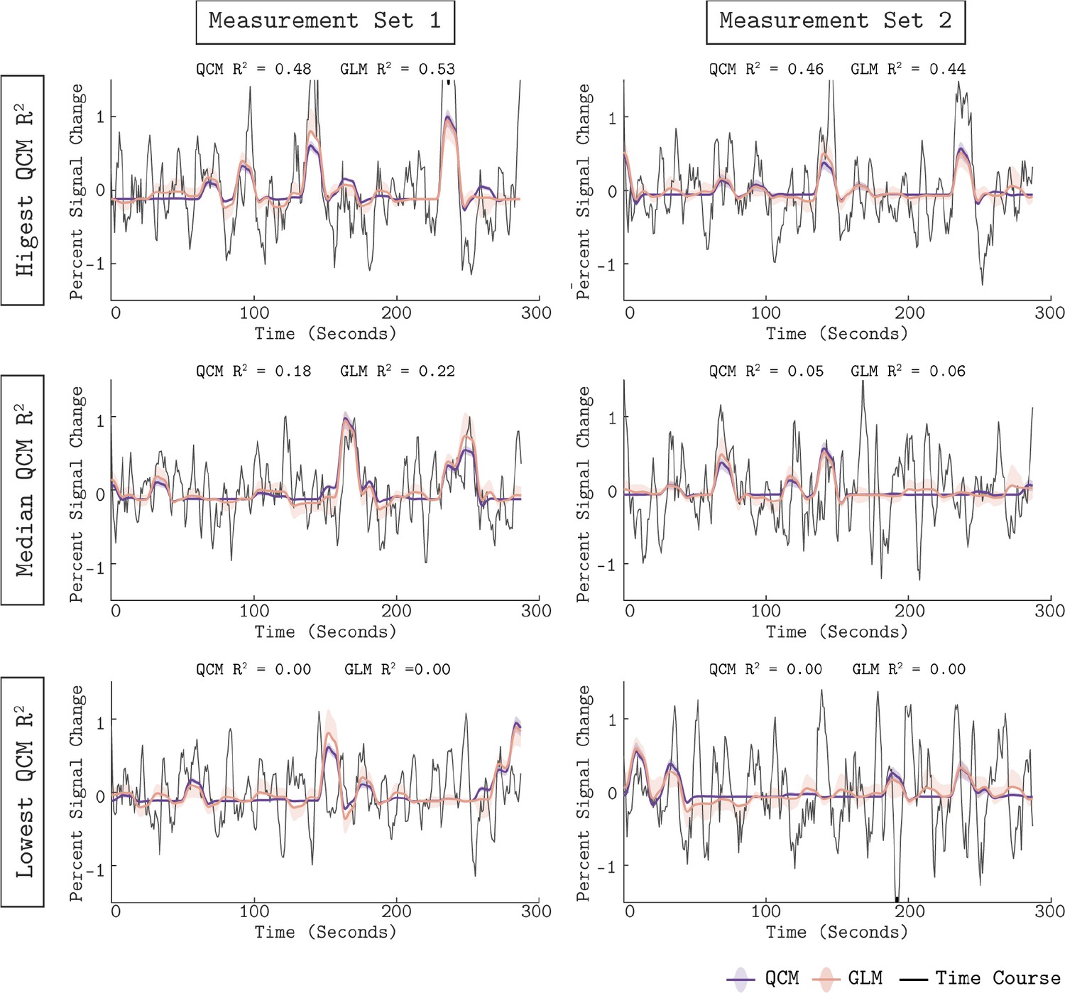
Model fits to the V1 BOLD time course from Subject 3.
The format of the figure is the same as Figure 3 in the main text and Figure 3—figure supplement 1 The measured BOLD time course (black line) is shown along with the model outputs from the QCM (thick purple line) and GLM (thin orange line) for six acquisitions.
Figure 3—figure supplement 3
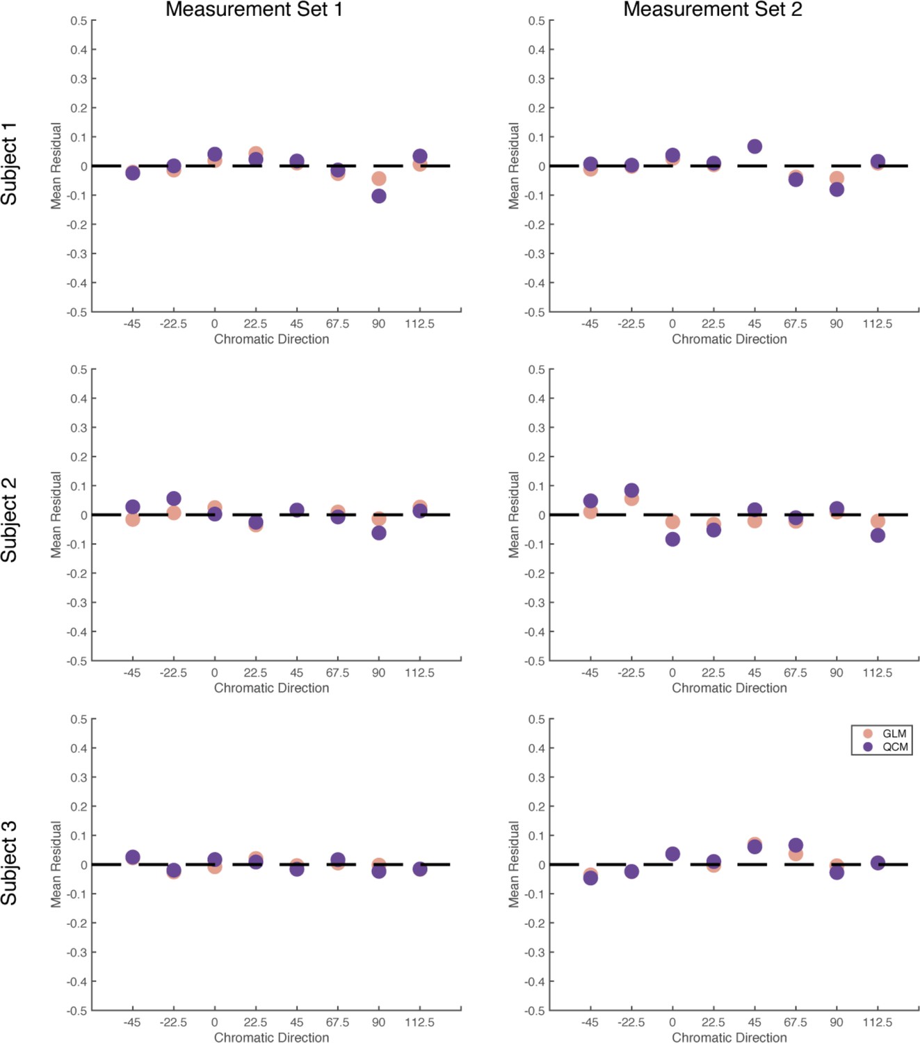
Mean Residuals for the QCM and the GLM.
Each panel shows the mean model residual for both the QCM (purple) and the GLM (orange) as a function of the chromatic direction. The mean of the model residuals is taken from 4 to 14 TRs after stimulus onset and is averaged for all stimuli within a color direction (collapsing over contrast). The rows show data for each of the three subjects and the columns show the two measument sets.
Figure 4 with 1 supplement
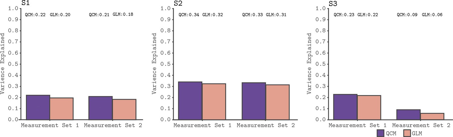
Cross-validated model comparison for the QCM and the GLM, from the V1 ROI and for all three subjects.
In each panel, the mean leave-one-out cross-validated R2 for the QCM (purple bars) and the GLM (orange bars). These values are displayed at the top of each panel. Within each panel, the left group is for Measurement Set 1 and the the right group is for Measurement Set 2.
Figure 4—figure supplement 1
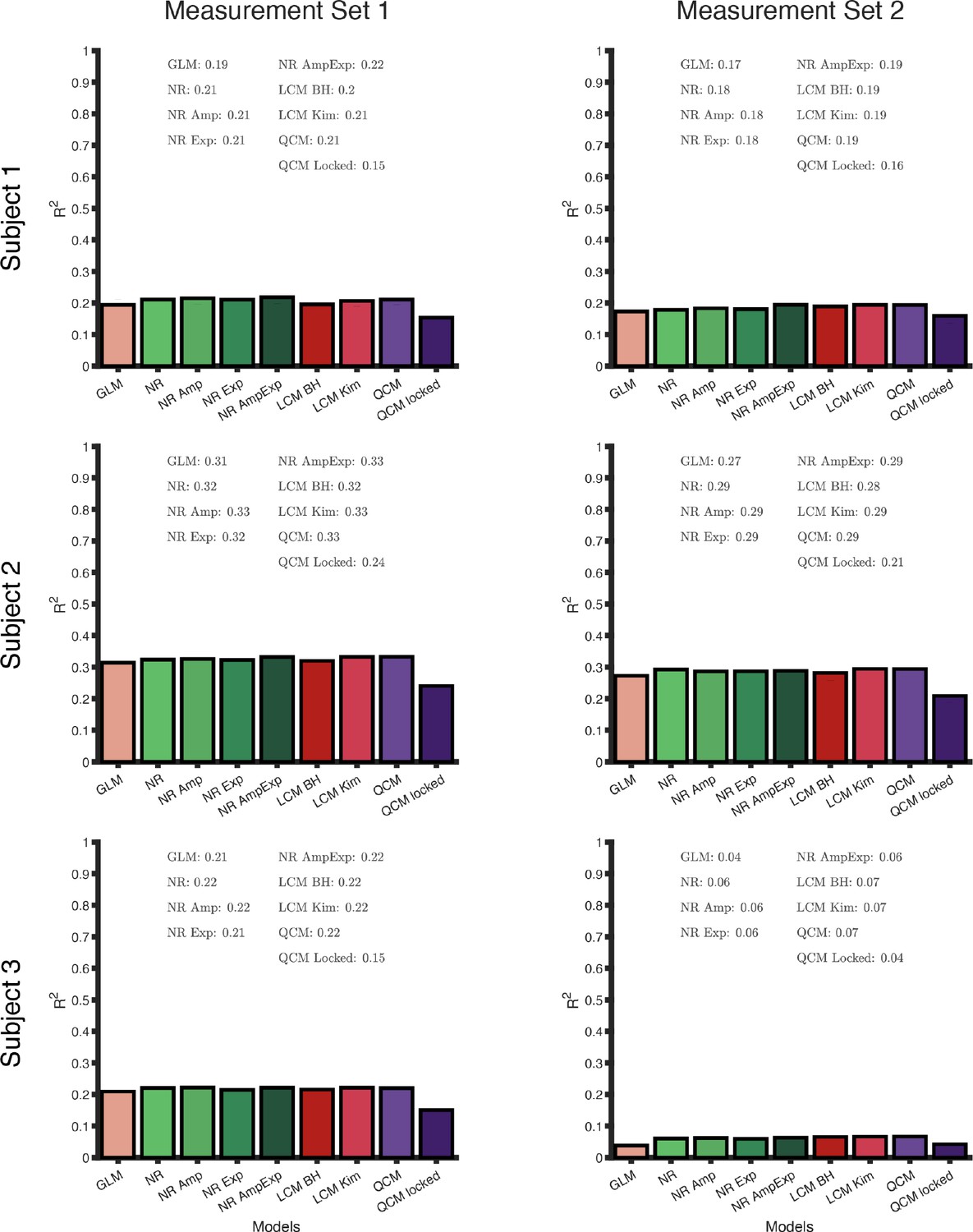
Cross-validated model comparison for all models, from the V1 ROI.
The rows show data for each subect and columns are the different measument sets. In each panel, we plot the mean leave-one-out cross-validated R2 (from left to right) for the General Linear Model, Naka-Rushton, Naka-Rushton common amplitude, Naka-Rushton common exponent, Naka-Rushton common amplitude and exponent, Linear Channels Model with Brouwer and Heeger parameters, Linear Channels Model with Kim et al. parameters, Quadratic Color Model, and Quadratic Color Model with angle locked to 0°. The cross-valided values are also provided numerically in the panels. Details for each model can be found in the main text and Appendix 1.
Figure 5 with 3 supplements

Leave-sessions-out cross validation.
The contrast response functions in each panel (green lines) are the result of a leave-sessions-out cross-validation to test the generalizability of the QCM. The QCM was fit to data from four out of the eight tested chromatic directions, either from Session 1 or Session 2. The fits were used to predict the CRFs for the held out four directions. The orange points in each panel are the GLM fits to the full data set. The data shown here are for Subject 2, Measurement Set 1. The shaded green error regions represent the 68% confidence intervals for the QCM prediction obtained using bootstrapping. See Figure 5—figure supplements 1–3 for cross-validation plots from other subjects and measurement sets.
Figure 5—figure supplement 1
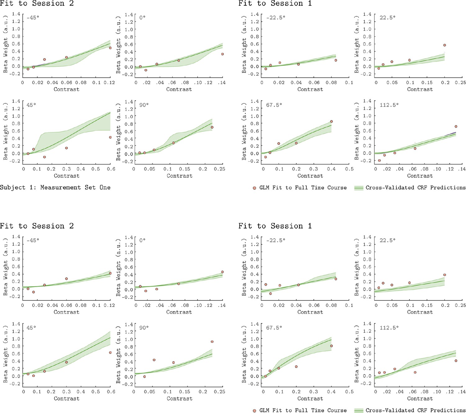
Leave-sessions-out cross validation for Subject 1.
The format of the Figure is the same as Figure 5 in the main text. The contrast response functions in each panel (green lines) are the result of a leave-sessions-out cross-validation to test the generalizability of the QCM. In both the top and bottom eight panels, the QCM was fit to data from four of the eight tested chromatic directions, either from session 1 or session 2. The fits were used to predict the CRFs for the held-out chromatic directions. The orange points in each panel are the GLM fits to the full data set. The data shown here are for Subject 1 with the top eight panels from Measurement Set 1 and the bottom eight panels from Measurement Set 2. The shaded green error regions represent the 68% confidence intervals for the QCM predictions obtained via the bootstrap analysis.
Figure 5—figure supplement 2
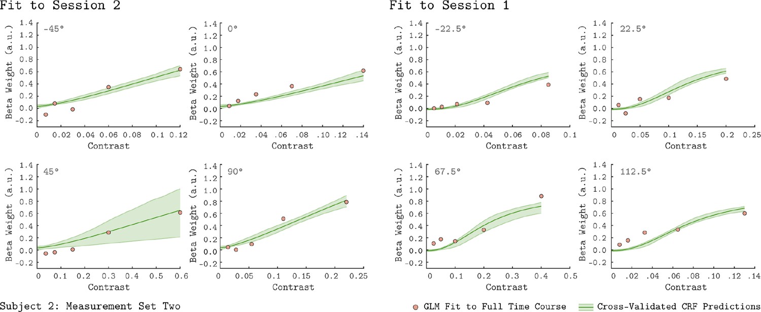
Leave-sessions-out cross validation for Subject 2.
The format of the figure is the same as Figure 5 in the main text and Figure 5—figure supplement 1. The contrast response functions in each panel (green lines) are the result of a leave-sessions-out cross-validation to test the generalizability of the QCM. The orange points in each panel are the GLM fits to the full data set. The data shown here are for Subject 2 Measurement Set 2; Measurement Set 1 can be seen in Figure 5 of the main text. The shaded green error regions represent the 68% confidence intervals for the QCM predictions obtained via the bootstrap analysis.
Figure 5—figure supplement 3
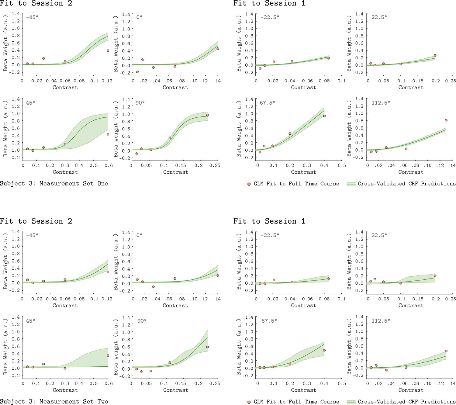
Leave-sessions-out cross validation for Subject 3.
The format of the figure is the same as Figure 5 in the main text and Figure 5—figure supplements 1–2. The green lines are the leave-session-out CRF, and the orange points are the GLM fits to the full data set. The data shown here are for Subject 3 with the top eight panels from Measurement Set 1 and the bottom eight panels from Measurement Set 2. The shaded green error regions represent the 68% confidence intervals for the QCM predictions obtained via the bootstrap analysis.
Figure 6 with 1 supplement

V1 isoresponse contours.
The normalized elliptical isoresponse contours from the QCM are plotted, for each subject, in the LM contrast plane. The green ellipses show the QCM fits to Measurement Set 1 and the purple ellipses show fits to measurement 2. The angles and minor axis ratios along with their corresponding 68% confidence intervals obtained using bootstrapping are provided in the upper left (Measurement Set 1) and lower right (Measurement Set 2) of each panel.
Figure 6—figure supplement 1
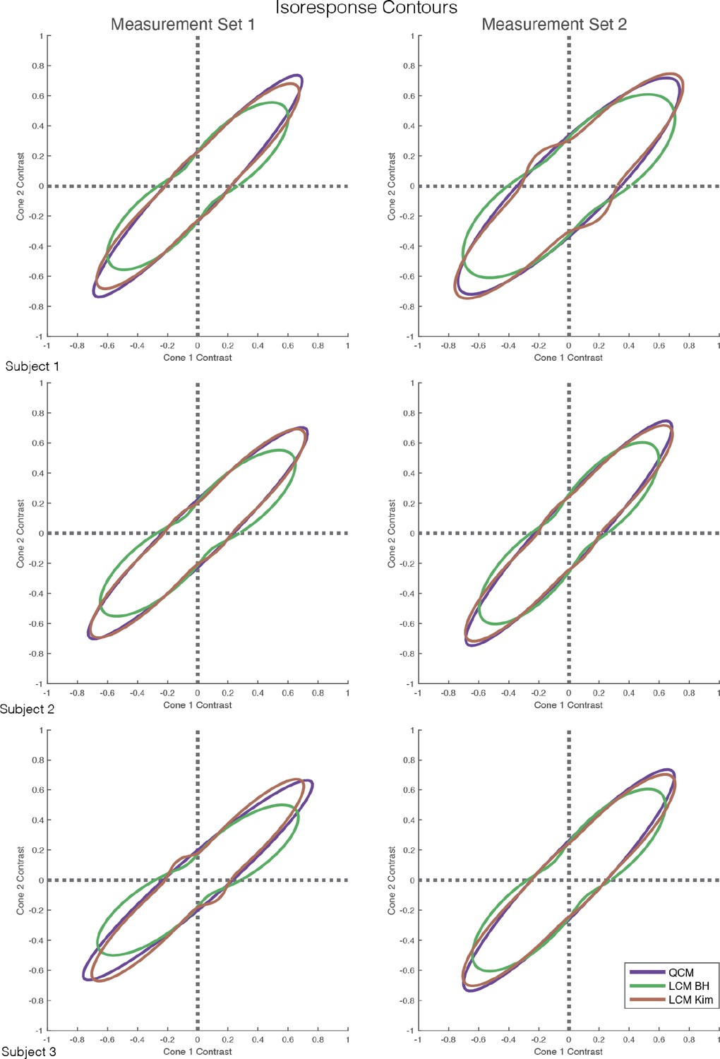
Isoresponse Contours for the LCM and the QCM.
Each panel shows the isoresponse contours derived using the LCM with both the Brouwer and Heeger, 2009 variant (green) and the Kim et al., 2020 (dark orange). These are shown along with the elliptical isoresponse contour from the corresponding QCM fit (purple). The rows show the fits to the data from each subject and the columns show the different measurement sets. Note that the isoresponse contour for the Kim et al., 2020 variant of the LCM, which has more degrees of freedom than the Brouwer and Heeger, 2009 variant, closely approximates that of the QCM.
Figure 7 with 1 supplement
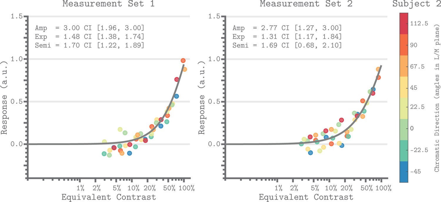
Equivalent contrast non-linearities of the QCM for V1 from Subject 2.
The x-axis of each panel marks the equivalent contrast and the y-axis is the neuronal response. The gray curve in each panel is the Naka-Rushton function obtained using the QCM fit. These curves show the relationship between equivalent contrast and response. The parameters of the Naka-Rushton function are reported in upper left of each panel along with the 68% confidence intervals obtained using bootstrapping. The points in each panel are the GLM beta weights mapped via the QCM isoresponse contours of Subject 2 onto the equivalent contrast axis (see Appendix 1). The color of each point denotes the chromatic direction of the stimuli, as shown in the color bar. The left panel is for Measurement Set 1 and the right panel is for Measurement Set 2. Note that our maximum contrast stimuli do not produce a saturated response. Note that our stimuli did not drive the response into the saturated regime.
Figure 7—figure supplement 1
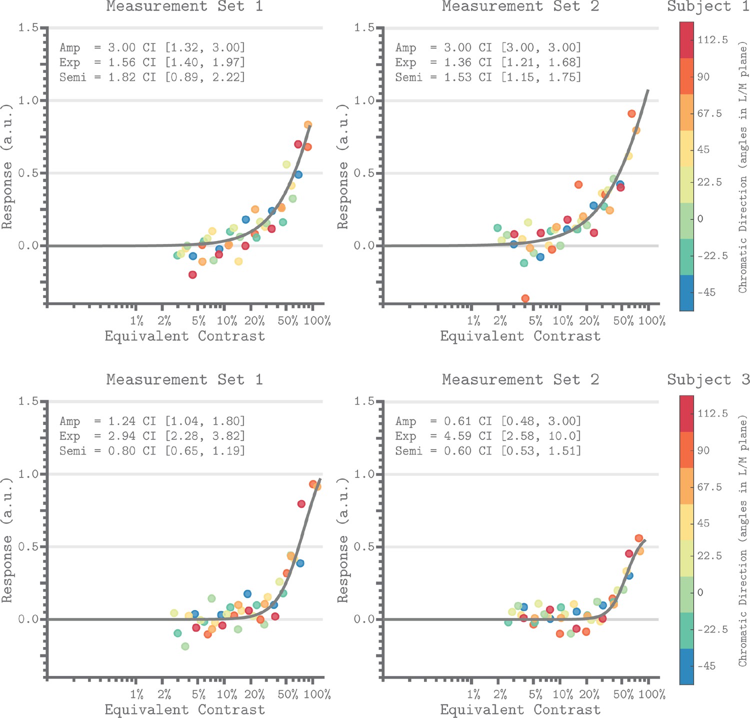
Equivalent Contrast Non-Linearities of the QCM for V1.
The format is the same as Figure 7 in the main text. The x-axis of each panel marks the equivalent contrast and the y-axis is the response. The gray curve in each panel is the Naka-Rushton function obtained using the QCM fit. The upper two panel are from Subject 1 and the bottom 2 panels are from Subject 3. The left panels are for Measurement Set 1 and the right panels are for Measurement Set 2. The parameters of the Naka-Rushton function are reported in upper left of each panel along with the 68% confidence intervals obtained via the bootstrap analysis. The points in each panel are the GLM beta weights of the respective measurement set mapped via the QCM isoresponse contours onto the equivalent contrast axis (see Materials and methods). The color of each point denotes the chromatic direction of the stimuli, as shown in the color bar.
Figure 8 with 1 supplement
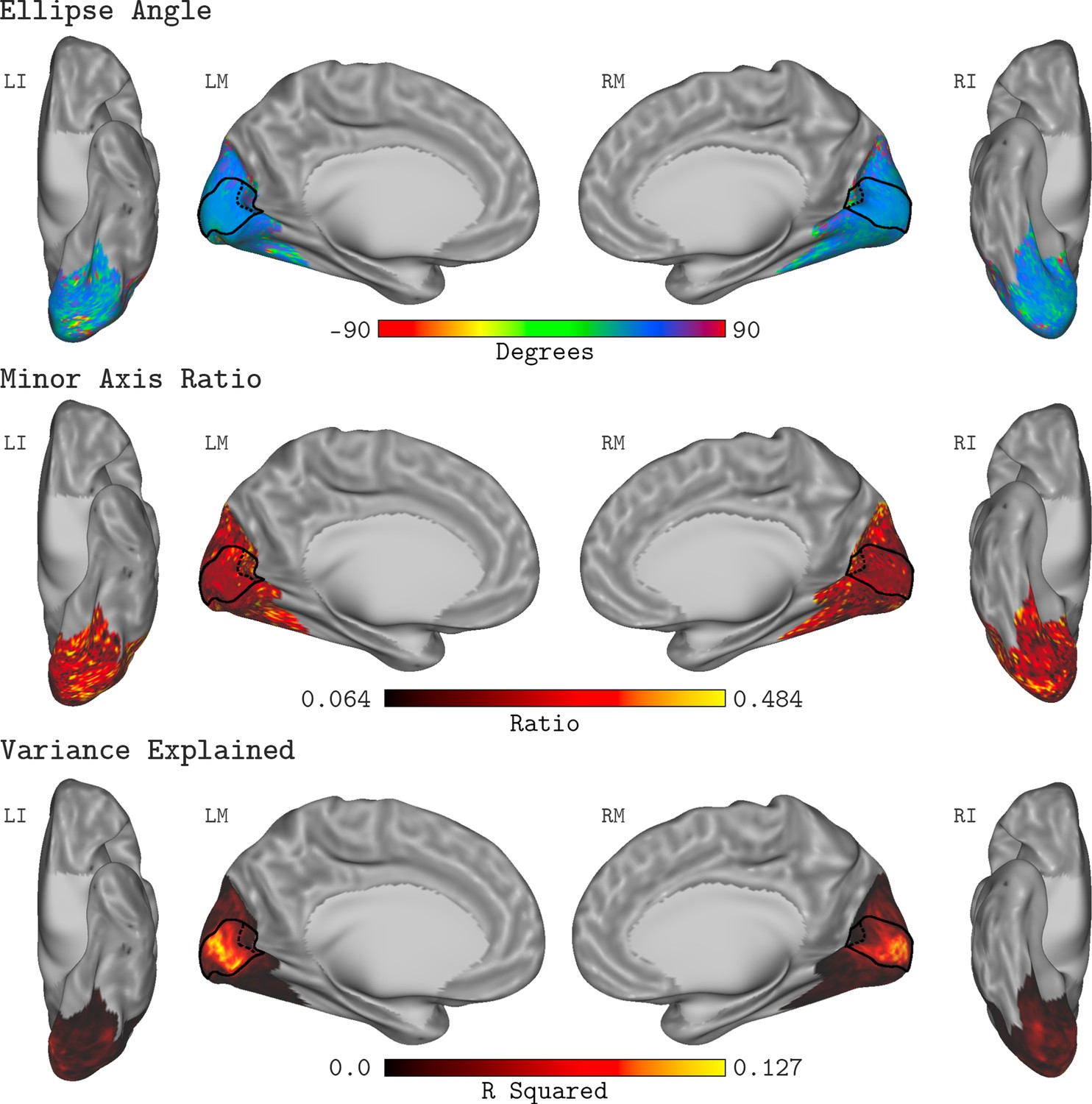
QCM average parameter maps.
The QCM parameters, fit at all vertices within the visual cortex mask, averaged across all subjects and measurement sets. The top, middle, and bottom rows show maps of the average ellipse angle, minor axis ratio, and variance explained, respectively. The scale of the corresponding color map is presented below each row. The nomenclature in upper left of each surface view indicates the hemisphere (L: left or R: right) and the view (I: inferior, L: lateral, or M: medial). The medial views show the full extent of the V1 ROI on the cortical surface (denoted by the solid black outline). The 20° eccentricity boundary used to define the V1 ROI used for all analyses is shown by the black dashed line.
Figure 8—figure supplement 1
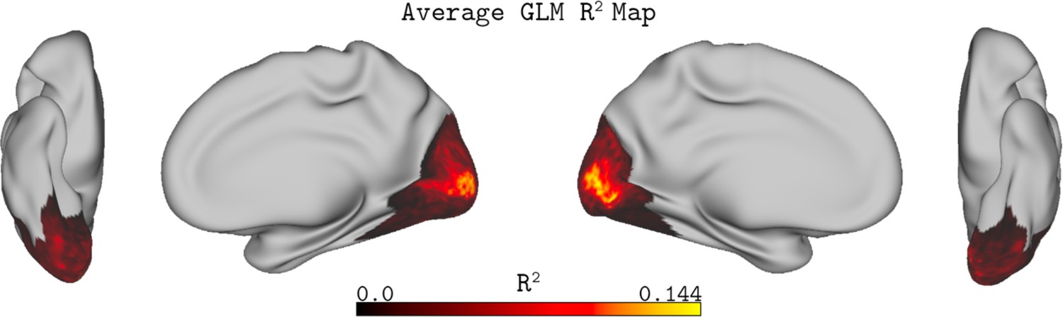
Average R2 map for the GLM for early visual cortex.
The format is the same as the bottom row of Figure 8 in the main text. This show the R2 values for the GLM fit to each vertex within the EVC mask averaged across all subjects and sessions. The color bar provides the GLM R2 scale.
Figure 9 with 2 supplements
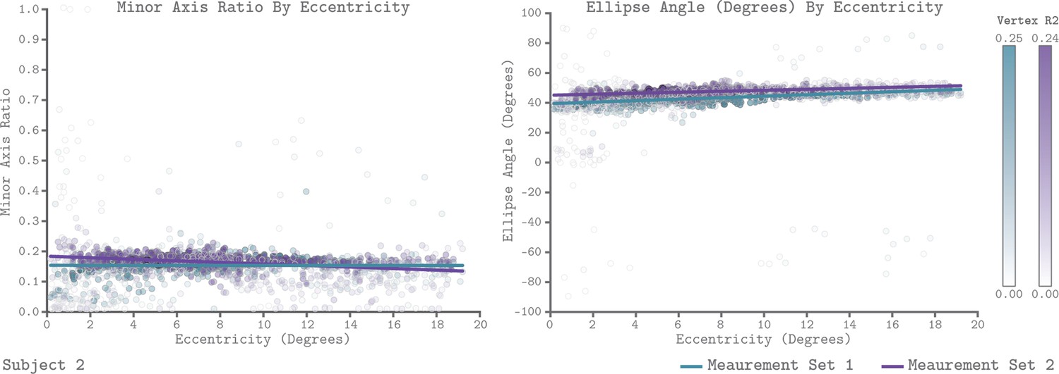
QCM parameters as a function of eccentricity for Subject 2.
The left and right panels show scatter plots of the minor axis ratio and ellipse angle plotted against their visual field eccentricity, respectively. Each point in the scatter plot shows a parameter value and corresponding eccentricity from an individual vertex. Green indicates Measurement Set 1 and purple indicates Measurement Set 2. The lines in each panel are robust regression obtained for each measurement set separately. The transparency of each point provides the R2 value of the QCM at that vertex. The color bars provide the R2 scale for each measurement set.
Figure 9—figure supplement 1
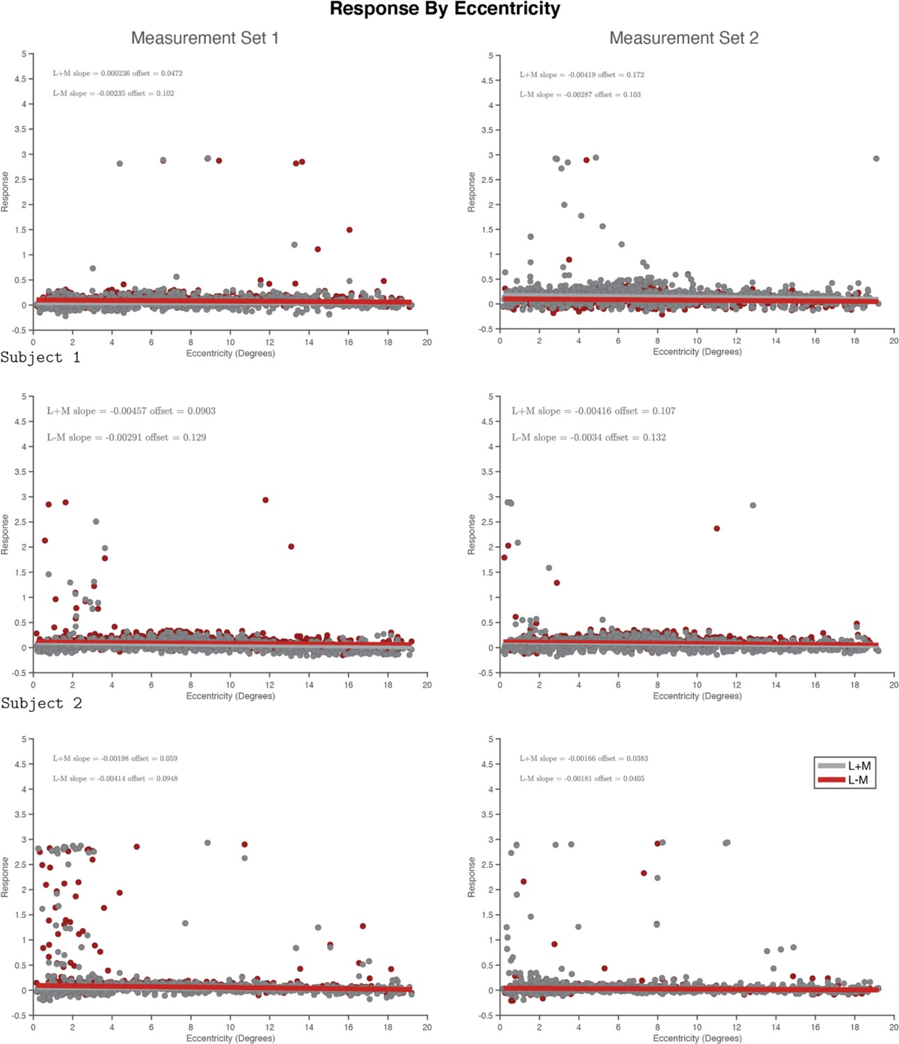
L+M and L-M responses predicted using QCM as a function of eccentricity.
The top row shows responses for Subject 1, the middle row show responses for Subject 2, and the bottom row shows responses for Subject 3. The left and right panels show data from Measurement Set 1 and Measurement Set 2, respectively. Each panel shows scatter plots of the QCM response for stimuli chosen in the L+M (gray) and L-M(red) directions plotted against their visual field eccentricity, respectively. The L+M stimulus was chosen at 6% contrast and the L-M stimulus was chosen at 30% contrast (corresponding to the 50% contrast condition). Note that a small percentage of vertices had poor parameter fits. Due to this, the predicted response amplitudes were orders of magnitude larger than what is currently displayed. These points have been excluded from the plot.
Figure 9—figure supplement 2
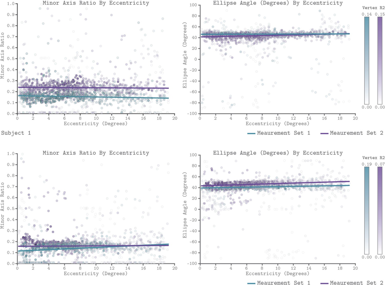
QCM parameters as a function of eccentricity.
The format is the same as Figure 9 in the main text. The top row shows parameter fits from Subject 1 and the bottom row shows fits from Subject 3. The left and right panels show scatter plots of the minor axis ratio and ellipse angle plotted against their visual field eccentricity, respectively. Each point in the scatter plot shows a parameter value and corresponding eccentricity from an individual vertex. Teal indicates Measurement Set 1 and purple indicates Measurement Set 2. The lines in each panel are robust regression obtained for each measurement set separately. The transparency of each point provides the R2 value of the QCM at that vertex. The color bars provide the R2 scale for each measurement set.
Figure 10

Stimulus space and temporal modulations.
(A) The LM contrast plane. A two-dimensional composed of axes that represent the change in L- and M-cone activity relative to the background cone activation, in units of cone contrast. Each aligned pair of vectors in this space represents the positive (increased activation) and negative (decreased activation) arms of the bipolar temporal modulations. We refer to each modulation by the angle of the positive arm in the LM contrast plane, with positive ∆L/L being at 0°. The black dashed lines show the maximum contrast used in each direction. The gray dashed circle shows 100% contrast. The ‘1’ or ‘2’ next to each positive arm denotes the session in which a given direction presented. The grouping was the same for Measurement Set 1 and Measurement Set 2. (B) The temporal profile of a single bipolar chromatic modulation. This shows how the cone contrast of a stimulus changed over time between the positive and negative arms for a given chromatic direction. The particular direction plotted corresponds to the 45° modulation at 12 Hz temporal frequency. The temporal profile was the same for all chromatic directions. (C) Schematic of the block structure of an functional run. Blocks lasted 12 s and all blocks were modulated around the same background. The amplitude of the modulation represents the contrast scaling, relative to its maximum contrast, for that block. Each run lasted a total of 288 s. The dark gray vertical bar represents an attentional event in which the light stimulus was dimmed for 500 ms.
Figure 11
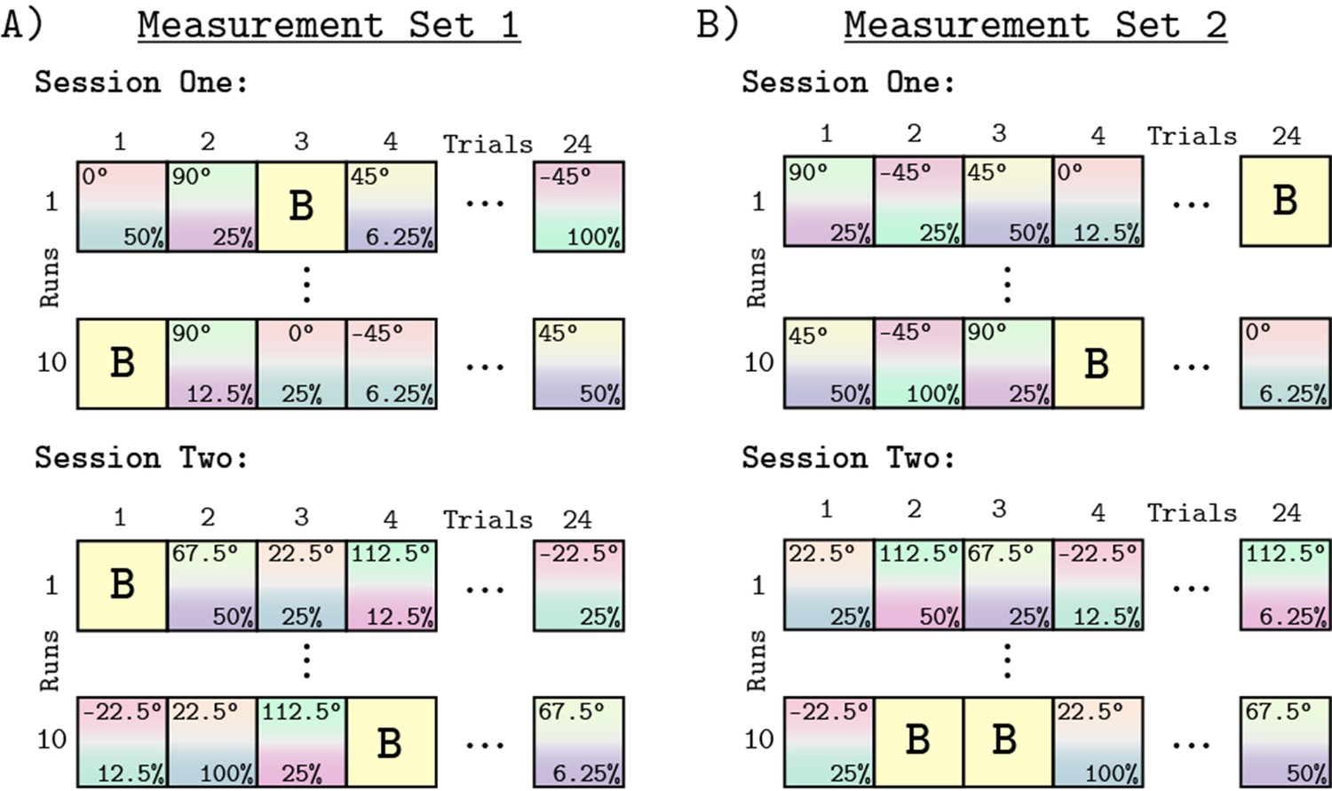
Experimental design.
Panels A and B show the block design used for all runs and sessions. Panel A shows Measurement Set 1 which contained two separate MRI sessions. Each session contained four of the eight chromatic directions. The split of directions across the two sessions was the same for all subjects, but which session each subject started with was randomized. Within a session we collected 10 functional runs, each containing 24 blocks. The 24 blocks consisted of 20 direction/contrast paired stimulus blocks (depicted by the gradient squares with direction noted at top and the contrast at bottom of each square) and 4 background blocks (squares marked 'B'). The order of blocks within each run was randomized, with each contrast/direction pair shown once per run. Each run had a duration of 288 second. Panel B shows Measurement Set 2, which was a replication of Measurement Set 1, with session order and order of blocks within run re-randomized. There were 960 blocks across both measurement sets.
Appendix 1—figure 1
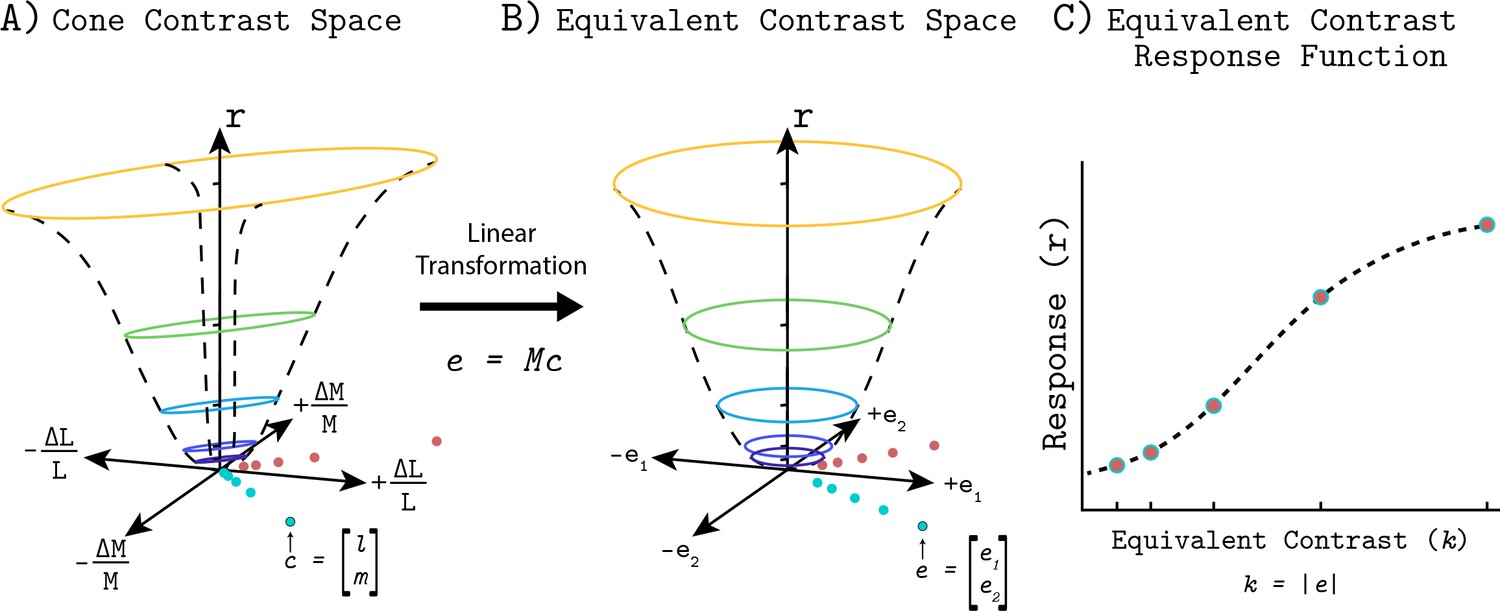
Illustration of cone to equivalent contrast transformation.
(Panel A) A 3-dimensional cone contrast-response space with the (,) plane representing the LM contrast plane and the axis giving the corresponding response to each point in the (,) plane. The teal and red dots shown in the LM plane represent example stimulus modulations, chosen in two color directions at contrasts corresponding to the five isoresponse contours illustrated in dark blue, blue, aqua, green, yellow. (Panel B) A three-dimensional equivalent contrast-response space with the (,) plane representing equivalent contrast (e1 and e2) and the axis giving the corresponding response to each point in the (,) plane. The teal and red dots shown correspond to same color dots in Panel A after we apply a linear transformation to (the L- and M-cone contrast representation of the stimuli) to obtain a transformed representation of the stimulus, . Note that after the application of , the elliptical contours in Panel A are circular and the distances between the plotted teal points are the same as the distances between the corresponding plotted red points. (Panel C) The equivalent contrast response function. The x-axis denotes the equivalent contrast and the y-axis marks the response. The teal and red closed circles shown in Panel C correspond to both the teal and red points shown in Panels A and B.
Author response image 1

Tables
Table 1
Robust regression line parameters summarizing the change in minor axis ratio with eccentricity for all subjects.
These parameters are the same as seen for Subject 2 in Figure 9. The subject and set columns indicate the subject and measurement set of the robust regression fit. The slope and offset column show the parameters of the regression line. The ∆ 0° to 20° column is the magnitude of the change in minor axis ratio between 0° and 20° eccentricity. The ∆ Set to Set column shows the absolute difference in the minor axis ratio fit to the V1 median time course between Measurement Set 1 and 2.
| Subject | Set | Slope | Offset | ∆ 0° to 20° | ∆ Set to Set |
|---|---|---|---|---|---|
| S1 | 1 | −1.19e-3 | 0.163 | 0.0238 | 0.09 |
| S1 | 2 | −4.17e-4 | 0.24 | 0.0084 | |
| S2 | 1 | −7.54e-6 | 0.154 | 0.0002 | 0.00 |
| S2 | 2 | −2.51e-3 | 0.183 | 0.0504 | |
| S3 | 1 | −3.27e-3 | 0.114 | 0.0654 | 0.03 |
| S3 | 2 | −3.9e-4 | 0.158 | 0.0078 |
Table 2
Robust regression line parameters summarizing the change in ellipse angle with eccentricity for all subjects.
Columns are formatted the same as Table 1.
| Subject | Set | Slope | Offset | ∆ 0° to 20° | ∆ Set to Set |
|---|---|---|---|---|---|
| S1 | 1 | 0.039 | 46.2 | 0.78 | 2.61 |
| S1 | 2 | 0.313 | 41.4 | 6.26 | |
| S2 | 1 | 0.496 | 39.5 | 9.92 | 3.76 |
| S2 | 2 | 0.330 | 45.1 | 6.60 | |
| S3 | 1 | 0.247 | 39.3 | 4.94 | 5.62 |
| S3 | 2 | 0.425 | 43.3 | 8.50 |
Table 3
Table of the nominal maximum contrast per direction.
The top row indicates the chromatic direction in the LM plane.The L, M, and S contrast rows show the desired contrast on the L, M, and S cones, respectively. The total contrast is the vectorlength of stimuli made up of the L, M, and S cone contrast components and is the definition of contrast used in this study.
| Direction | −45° | −22.5° | 0° | 22.5° | 45° | 67.5° | 90° | 112.5° |
|---|---|---|---|---|---|---|---|---|
| L-Contrast | 8.49% | 7.85% | 14% | 18.48% | 42.43% | 15.31% | 0% | 4.98% |
| M-Contrast | 8.49% | 3.25% | 0% | 7.65% | 42.43% | 36.96% | 22% | 12.01% |
| S-Contrast | 0% | 0% | 0% | 0% | 0% | 0% | 0% | 0% |
| Total Contrast | 12% | 8.5% | 14% | 20% | 60% | 40% | 22% | 13% |
Table 4
Number of censored fMRI frames per run.
Values shown are for Subject 1 Measurement Set 2. The top set of rows show data for session one and the bottom set of the show data for session 2. Each set of rows show the number of censored frames per run out of 360 frames. Subjects and sessions not shown mean that no frames were censored in those runs.
| Subject 1 – Measurement Set 2: Session 1 | ||||||||||
|---|---|---|---|---|---|---|---|---|---|---|
| Run Number | 1 | 2 | 3 | 4 | 5 | 6 | 7 | 8 | 9 | 10 |
| Number of Censored Frames (n/360) | 0 | 0 | 8 | 18 | 0 | 26 | 47 | 4 | 0 | 0 |
| Subject 1 – Measurement Set 2: Session 2 | ||||||||||
| Run Number | 1 | 2 | 3 | 4 | 5 | 6 | 7 | 8 | 9 | 10 |
| Number of Censored Frames (n/360) | 0 | 0 | 0 | 0 | 0 | 0 | 0 | 7 | 0 | 0 |
Table 5
Stimulus validation measurements for Subject 1.
The top set of rows show data for Measurement Set 1 and the bottom set show data for Measurement Set 2. The dark gray rows show the nominal angle and contrast. Each cell shows the mean and standard deviation of stimulus vector angles and lengths computed from 10 validation measurements (5 pre-experiment, 5 post-experiment). Center and periphery denote which set of cone fundamentals were used to calculate cone contrast of the stimuli referring either the 2° or 15° CIE fundamentals, respectively.
| Subject 1 – Measurement Set 1 | ||||||||
|---|---|---|---|---|---|---|---|---|
| Nominal Angle | −45° | −22.5° | 0° | 22.5° | 45° | 67.5° | 90° | 112.5° |
| Center Angle | −41.23 ±3.13 | −15.90 ±6.59 | 2.17 ±1.05 | 23.43 ±0.23 | 45.21 ±0.23 | 69.36 ±1.61 | 87.98 ±1.26 | 120.94 ±8.45 |
| Periphery Angle | −42.85 ±3.04 | −16.31 ±6.18 | 1.61 ±0.44 | 22.75 ±0.22 | 44.78 ±0.22 | 68.13 ±1.54 | 88.72 ±0.18 | 119.67 ±8.04 |
| Nominal Contrast | 12% | 8.5% | 14% | 20% | 60% | 40% | 22% | 13% |
| Center Contrast | 12.14 ±0.05 | 9.02 ±0.75 | 14.44 ±0.37 | 21.05 ±0.79 | 60.92 ±0.09 | 38.01 ±1.97 | 21.39 ±0.85 | 12.56 ±0.38 |
| Periphery Contrast | 12.00 ±0.04 | 8.93 ±0.72 | 13.98 ±0.35 | 20.28 ±0.73 | 58.73 ±0.09 | 37.81 ±1.89 | 21.42 ±0.55 | 12.48 ±0.36 |
| Subject 1 - Measurement Set 2 | ||||||||
| Nominal Angle | −45° | −22.5° | 0° | 22.5° | 45° | 67.5° | 90° | 112.5° |
| Center Angle | −45.09 ±0.55 | −22.44 ±0.98 | 3.49 ±2.27 | 22.97 ±0.15 | 45.18 ±0.03 | 67.75 ±0.24 | 87.81 ±1.69 | 112.99 ±1.03 |
| Periphery Angle | −46.16 ±0.55 | −22.32 ±0.99 | 3.24 ±2.77 | 22.39 ±0.19 | 44.92 ±0.02 | 66.85 ±0.21 | 87.33 ±1.24 | 68.34 ±0.92 |
| Nominal Contrast | 12% | 8.5% | 14% | 20% | 60% | 40% | 22% | 13% |
| Center Contrast | 11.75 ±0.01 | 8.28 ±0.08 | 13.78 ±0.09 | 20.35 ±0.22 | 60.26 ±0.48 | 37.62 ±0.11 | 21.82 ±0.08 | 12.69 ±0.05 |
| Periphery Contrast | 11.65 ±0.02 | 8.29 ±0.08 | 13.53 ±0.09 | 19.79 ±0.18 | 58.47 ±0.48 | 38.16 ±0.10 | 21.99 ±0.10 | 12.81 ±0.06 |
Table 6
Stimulus validation measurements for Subject 2.
The format of this table is the same as Table 5. Cells that contain an 'X' mark stimulus directions in which validation measurements were not recorded due to technical difficulty.
| Subject 2 - Measurement Set 1 | ||||||||
|---|---|---|---|---|---|---|---|---|
| Nominal Angle | −45° | −22.5° | 0° | 22.5° | 45° | 67.5° | 90° | 112.5° |
| Center Angle | −45.73 ±1.06 | −19.23 ±2.51 | 1.71 ±0.98 | 24.04 ±0.39 | 45.43 ±0.09 | 68.36 ±0.53 | 87.87 ±1.64 | 114.92 ±1.90 |
| Periphery Angle | −47.03 ±1.02 | −18.91 ±2.40 | 1.63 ±0.77 | 23.65 ±0.38 | 44.99 ±0.09 | 67.18 ±0.52 | 87.65 ±1.09 | 114.11 ±1.86 |
| Nominal Contrast | 12% | 8.5% | 14% | 20% | 60% | 40% | 22% | 13% |
| Center Contrast | 12.04 ±0.11 | 8.41 ±0.21 | 14.01 ±0.08 | 20.45 ±0.52 | 60.72 ±0.38 | 39.68 ±0.63 | 21.82 ±0.23 | 12.73 ±0.16 |
| Periphery Contrast | 11.88 ±0.11 | 8.36 ±0.21 | 13.58 ±0.07 | 19.81 ±0.51 | 58.56 ±0.35 | 39.41 ±0.59 | 21.82 ±0.24 | 12.62 ±0.14 |
| Subject 2 - Measurement Set 2 | ||||||||
| Nominal Angle | −45° | −22.5° | 0° | 22.5° | 45° | 67.5° | 90° | 112.5° |
| Center Angle | X | −25.85 ±3.20 | X | 22.72 ±0.38 | X | 67.42 ±0.16 | X | 112.03 ±1.22 |
| Periphery Angle | X | −26.43 ±3.04 | X | 22.35 ±0.35 | X | 66.36 ±0.16 | X | 110.12 ±1.17 |
| Nominal Contrast | 12% | 8.5% | 14% | 20% | 60% | 40% | 22% | 13% |
| Center Contrast | X | 8.36 ±0.16 | X | 19.77 ±0.23 | X | 39.75 ±0.13 | X | 12.75 ±0.15 |
| Contrast | X | 8.34 ±0.17 | X | 19.21 ±0.23 | X | 40.04 ±0.15 | X | 12.95 ±0.13 |
Table 7
Stimulus validation measurements for Subject 3.
| Subject 3 - Measurement Set 1 | ||||||||
|---|---|---|---|---|---|---|---|---|
| Nominal Angle | −45° | −22.5° | 0° | 22.5° | 45° | 67.5° | 90° | 112.5° |
| Center Angle | −48.84 ±5.02 | −27.84 ±6.02 | 5.29 ±4.45 | 23.61 ±0.77 | 45.41 ±0.15 | 67.48 ±0.42 | 85.96 ±3.11 | 108.56 ±4.89 |
| Periphery Angle | −50.40 ± 4.90 | −28.48 ±5.97 | 5.09 ±4.72 | 23.26 ±0.77 | 45.02 ±0.13 | 66.33 ±0.43 | 86.12 ±3.24 | 107.49 ±4.78 |
| Nominal Contrast | 12% | 8.5% | 14% | 20% | 60% | 40% | 22% | 13% |
| Center Contrast | 12.25 ±0.32 | 8.39 ±0.06 | 13.96 ±0.08 | 19.78 ±0.20 | 61.92 ±1.40 | 40.87 ±1.14 | 22.91 ±1.30 | 13.53 ±0.75 |
| Periphery Contrast | 12.13 ±0.31 | 8.30 ±0.08 | 13.52 ±0.09 | 19.17 ±0.21 | 59.76 ±1.36 | 40.65 ±1.13 | 22.97 ±1.26 | 13.47 ±0.71 |
| Subject 3 - Measurement Set 2 | ||||||||
| Nominal Angle | −45° | −22.5° | 0° | 22.5° | 45° | 67.5° | 90° | 112.5° |
| Center Angle | X | −24.51 ±1.57 | X | 22.92 ±0.07 | X | 67.65 ±0.19 | X | 111.23 ±1.11 |
| Periphery Angle | X | −24.17 ±1.53 | X | 22.65 ±0.06 | X | 66.57 ±0.19 | X | 69.95 ±1.07 |
| Nominal Contrast | 12% | 8.5% | 14% | 20% | 60% | 40% | 22% | 13% |
| Center Contrast | X | 8.24 ±0.07 | X | 19.93 ±0.09 | X | 39.77 ±.0.27 | X | 12.88 ±0.11 |
| Periphery Contrast | X | 8.23 ±0.07 | X | 19.45 ±0.26 | X | 40.16 ±0.26 | X | 12.92 ±0.10 |
Additional files
Download links
A two-part list of links to download the article, or parts of the article, in various formats.
Downloads (link to download the article as PDF)
Open citations (links to open the citations from this article in various online reference manager services)
Cite this article (links to download the citations from this article in formats compatible with various reference manager tools)
A quadratic model captures the human V1 response to variations in chromatic direction and contrast
eLife 10:e65590.
https://doi.org/10.7554/eLife.65590


