Understanding the evolution of multiple drug resistance in structured populations
- Centre D'Ecologie Fonctionnelle & Evolutive, CNRS, Univ Montpellier, EPHE, IRD, France
Figures
Figure 1
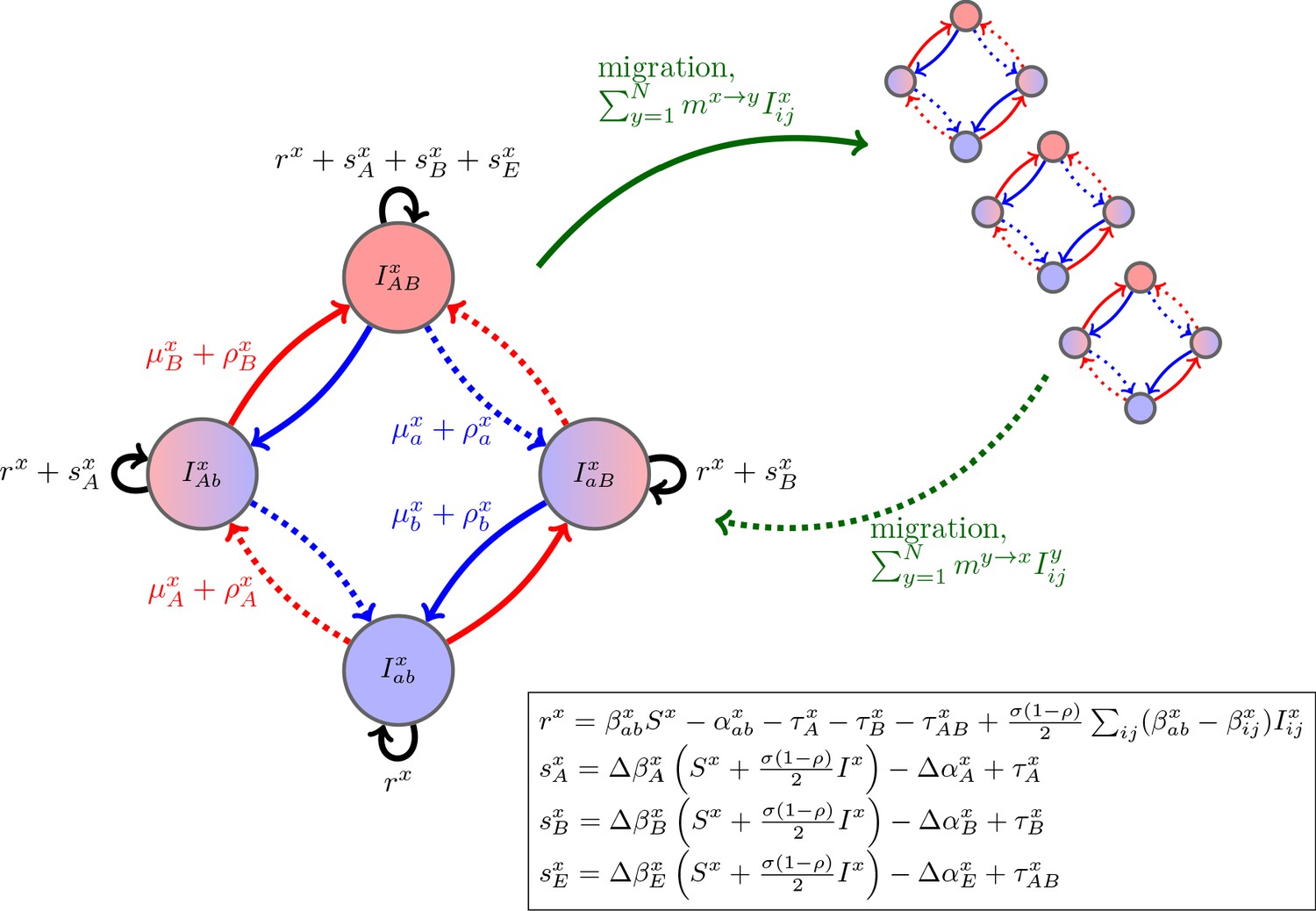
Schematic of the dynamics of system (2).
The metapopulation consists of connected populations. Each population has four possible types of infections, linked by one-step mutation or recombination (blue and red arrows), whose per-capita rates are independent of genetic background. The ‘baseline’ per-capita growth rate of sensitive infections is , the additive selection coefficients for drug and resistance are and , respectively, while denotes any epistatic interactions. In the inset, we compute these quantities for the specific model introduced in the main text, using the notation that and are the contribution of trait to the additive selection coefficient (for resistance to drug ) and to epistasis, respectively, in population (e.g., and ).
Figure 2
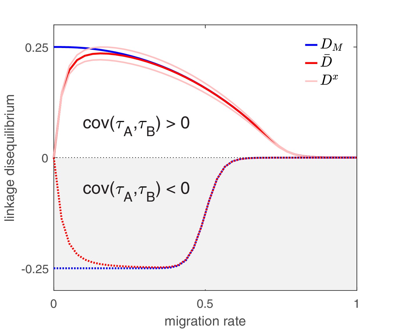
The effect of migration upon LD at equilibrium depends upon the scale at which LD is measured.
Here, we show equilibrium LD in a metapopulation consisting of four populations. Two scenarios are shown. In the first scenario (solid lines), drug and drug are both prescribed in the same two populations while the other two populations receive no drugs, thus ; this yields and so positive population, average, and metapopulation LD, that is, . In the second scenario (dashed lines), drug is prescribed in two populations and drug is prescribed in the other two populations, thus ; this yields and negative population, average, and metapopulation LD, i.e., . Because we assume identical treatment rates and costs of resistance for either drug, in the second scenario all the populations have the same LD, whereas in the first scenario, since the drugs are prescribed unequally across populations, the LD observed in each of the two pairs of populations diverge. Specifically, populations experiencing greater selection due to increased drug prescription also have greater LD; this follows from the first term in Equation (4).
Figure 3
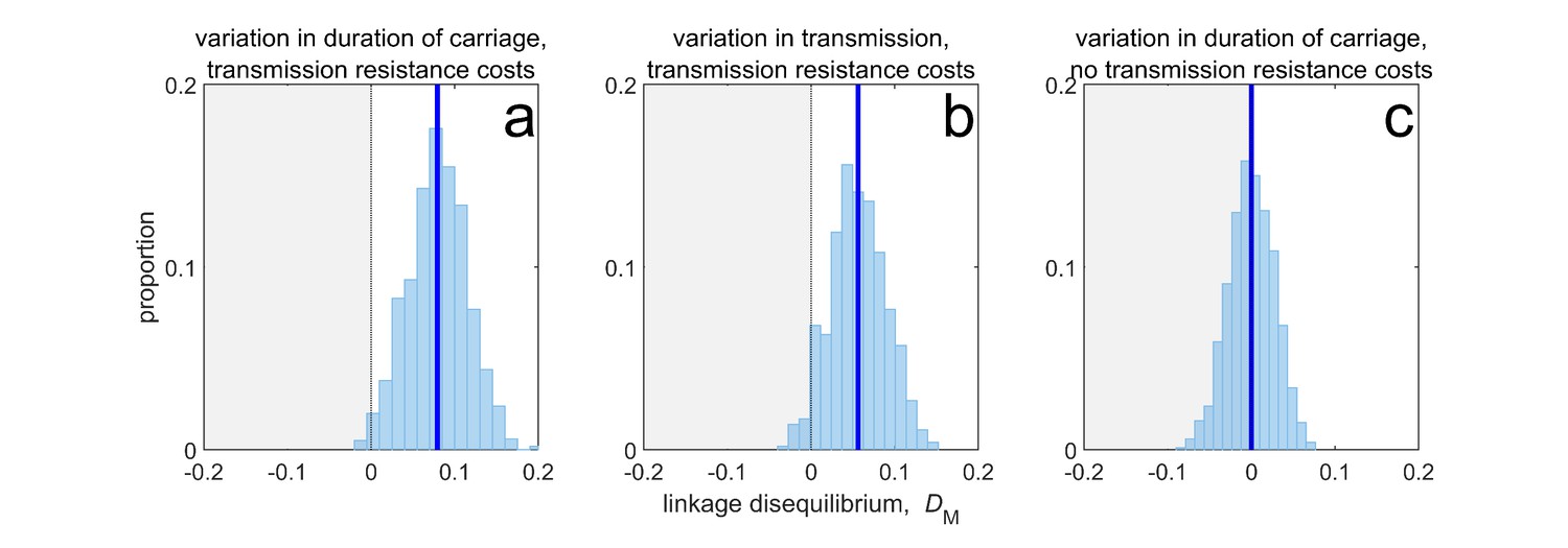
Duration of carriage is one of many potential explanations for MDR over-representation at equilibrium.
When costs are additive and there is no epistasis, variation in duration of carriage across independent populations can lead to linkage disequilibrium (subplot a), but it is neither necessary (b), nor sufficient (c). We simulate 1000 populations (blue bars), each consisting of 20 independent populations in which treatment rates for each population are randomly chosen to be either or with equal probability while simultaneously satisfying . The solid blue line is the mean LD across the simulations for each scenario. In subplot a, duration of carriage varies across populations and there are transmission resistance costs; in subplot b, transmission varies and there are transmission resistance costs; while in subplot c, duration of carriage varies and there are no transmission costs. These simulations diverge slightly from those of Lehtinen et al., 2019 in that their model always includes epistasis (see Materials and methods 'Equilibrium analysis of metapopulation consisting of independent populations'), whereas here we only consider non-epistatic scenarios.
Figure 4
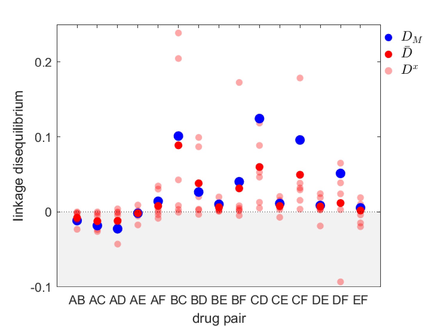
Linkage disequilibrium for different drug pairs in Streptococcus pneumoniae.
Data is from the Maela surveillance data set of Lehtinen et al., 2019; Turner et al., 2012. The light red circles are the observed serotype LD, , the dark red circles are the average LD across serotypes, , while the blue circles are the metapopulation LD, . We have restricted the data to serotypes involving 100 or more samples (serotypes 14, 6A/C, 6B, 15B/C, 19F, 23F). The drugs considered are: A = chloramphenicol, B = clindamycin, C = erythromycin, D = penicillin, E = sulphatrimethoprim, and F = tetracycline.
Figure 5
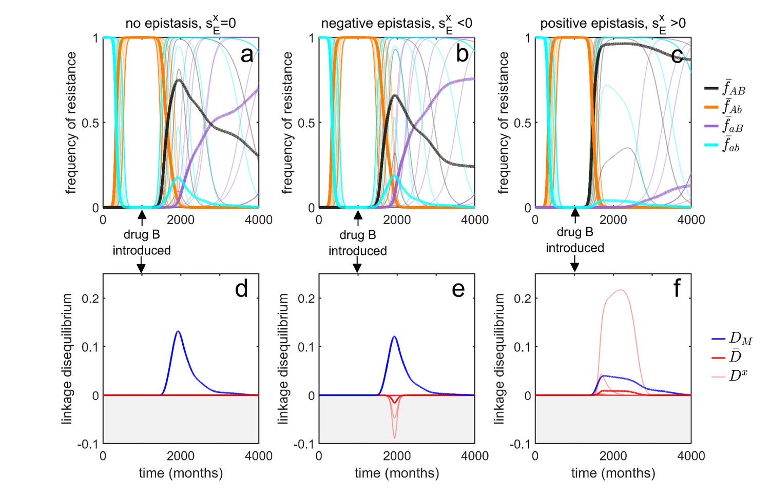
Transient dynamics coupled with epistasis can explain patterns of serotype LD in Streptococcus pneumoniae.
In all simulations, serotypes differ based upon duration of carriage and transmissibility. At , the pathogen is sensitive to both drugs; however, as hosts are initially treated with drug at a rate of per month, resistance to drug emerges and fixes in all serotypes. At (months), drug is introduced, and drug prescription reduced, (note that the drugs are never prescribed in combination, ). In the first column, there is no epistasis, thus although metapopulation LD builds up, serotype LD does not. In the second column, there is negative epistasis, which generates negative serotype LD. In the third column, there is positive epistasis which produces positive serotype LD. The thin lines denote the within-serotype dynamics, while the thick lines denote the metapopulation dynamics. In all cases, at equilibrium both the serotypes and the metapopulation will be in linkage equilibrium, however, transient LD can occur on sufficiently long timescales so as to appear permanent (see Materials and methods 'Transient dynamics and MDR in streptococcus pneumoniae' for more details).
Figure 6
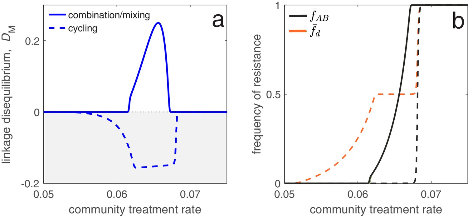
Different antibiotic prescription strategies generate different patterns of LD at equilibrium.
Here, we focus upon a population divided into a community and a hospital. Individuals enter the hospital at a fixed rate and spend a fifth of the time in the hospital that it takes to naturally clear a sensitive infection. The hospital/community size split corresponds to 20 beds per 1000 people, while individuals in the hospital receive antibiotics at 15x the rate they do in the community. We integrate system (2) until equilibrium is reached; the final state of the system is what is shown. For cycling, we compute the average state over the last two rotations (i.e., over the last period, ; in this case ). In panel a, we show the metapopulation LD, for the three treatment scenarios (combination, mixing, cycling). Combination and mixing generate identical LD in this example. In panel b we show the frequency of infections in the metapopulation resistant to drug , (for our choice of parameters, ; Materials and methods 'Contrasting drug prescription strategies in a hospital-community setting'), and doubly-resistant, , for each scenario. Note that for mixing and combination treatments (solid curves), , whereas cycling (dashed curves) leads to singly-resistant infections at low treatment rates (see Materials and methods 'Contrasting drug prescription strategies in a hospital-community setting').
Figure 7

Time between drug rotations affects the evolution of both single- and multi-drug resistance.
When drugs are rotated every 0.5 time units (period of ; magenta curves), cycling behaves like mixing and positive LD is generated. As we increase the time between rotations (period of and ), a negative covariance in selection is generated, producing negative LD (dashed and solid blue curves). In panel a we show the metapopulation LD, , while in panel b, we show the frequency of resistance in the metapopulation. When drugs are rotated frequently, single drug resistance emerges at higher treatment rates but MDR emerges at lower treatment rates, as compared to when drugs are rotated infrequently. Thus, there is a trade-off (indicated by the arrows in panel b) associated with time between drug rotations: we can delay single drug resistance but promote MDR (frequent drug rotations), or delay MDR but promote single drug resistance (infrequent drug rotations). In all cases, we integrated the system until , then averaged the system state over the final two rotations (i.e. over a single period). The remaining parameter values are provided in Materials and methods 'Contrasting drug prescription strategies in a hospital-community setting'.
Tables
Table 1
Notation used in main text.
In all cases, a quantity indexed with a superscript is the population quantity, whereas the absence of a superscript implies the quantity is for the metapopulation.
| Symbol | Description |
|---|---|
| Density of -infections in population , where (resp. ) if infection is resistant (resp. sensitive) to drug and (resp. ) if infection is resistant (resp. sensitive) to drug . | |
| Density of total infections in population . | |
| , | Frequency of infections resistant to drug in population and the metapopulation, respectively. |
| , , | Linkage disequilibrium (LD) in population , average LD across populations and metapopulation LD, respectively. |
| Per-capita rate at which hosts migrate from population to . | |
| , | Per-capita growth rate of sensitive infections in population (or ‘baseline’ per-capita growth rate) and average across populations, respectively. |
| , | Additive selection coefficient for resistance to drug in population and average selection across populations, respectively. |
| , | Epistasis in fitness across drug resistance loci in population and average across populations, respectively. |
| , | Net change in -infections in population due to mutation or recombination, respectively. |
| , | Per-capita rate at which mutations generate allele in population and average across populations, respectively. |
| , | Per-capita rate at which recombination leads to gain of allele in population and average across populations, respectively. |
| , | Average selection for drug resistance in population and average across populations, respectively. |
| Covariance between the variables and , that is, , where denotes the expectation of quantity . | |
| Coskewness between the quantities , , , that is, . |
Additional files
Download links
A two-part list of links to download the article, or parts of the article, in various formats.
Downloads (link to download the article as PDF)
Open citations (links to open the citations from this article in various online reference manager services)
Cite this article (links to download the citations from this article in formats compatible with various reference manager tools)
Understanding the evolution of multiple drug resistance in structured populations
eLife 10:e65645.
https://doi.org/10.7554/eLife.65645


