Multiple time-scales of decision-making in the hippocampus and prefrontal cortex
- Graduate Program in Neuroscience, Brandeis University, United States
- Neuroscience Program, Department of Psychology, and Volen National Center for Complex Systems, Brandeis University, United States
Figures
Figure 1 with 1 supplement

Choice-specific sequences in CA1 and PFC during memory-guided navigation decisions.
(A) Diagrams of two possible past (inbound; left) and future (outbound; right) scenarios during a W-maze spatial alternation task. In this task, rats have to remember their past choice between two possible locations (Left vs. Right arms; left), and then choose the opposite arm correctly (right; see Materials and methods). CP: choice point. (B) Behavioral performance of all nine rats that learned the inbound (IN; green) and outbound (OUT; blue) components of the task over eight sessions within a single day. Dashed lines: individual animals. Thick lines with error bars: means with SEMs. Horizontal dashed lines: chance-level of 0.5. Prob.: probability. (C) Simultaneously recorded ensembles of CA1 and PFC cells, forming slow behavioral sequences spanning the entire trajectory (~8 s), fast replay sequences (~260 ms; brown shading), and fast theta sequences (~100–200 ms; blue shadings). Each row represents a cell ordered and color-coded by spatial-map center on the Center-to-Left (C–to–L) trajectory shown top right. Gray lines: actual position. Dashed vertical line: reward well exit. Black, brown, and dark blue lines: broadband, ripple-band, and theta-band filtered LFPs from one CA1 tetrode, respectively. (D–I) Choice-predictive representations of behavioral sequences in CA1 and PFC. (D and E) Four trajectory-selective example cells during (D) outbound and (E) inbound navigation (shadings: SEMs; black arrowheaded line indicates animal’s running direction). (F and G) Example choice-specific behavioral sequences. For each plot pair, the top illustrates a raster of trajectory-selective cell assemblies ordered by spatial-map centers on the preferred trajectory; the bottom shows population decoding of animal’s choice and locations at the behavioral timescale (bin = 120 ms; note that summed probability of each column across two trajectory types is 1). Green and yellow arrowheads indicate the example cells shown in (D) and (E). Color bar: posterior probability. Green lines: actual position. Blue and red arrowheads: the CP. Note that the rasters only show trajectory-selective cells, whereas the population decoding was performed using all cells recorded in a given region. (H and I) Behavioral sequences in (H) CA1 and (I) PFC predicted current choices. Left: decoding accuracy of current choice over locations (n = 9 rats×8 sessions); Right: decoding accuracy of current choice on the center stem across sessions. Note that the decoding performance is significantly better than chance (50%) over locations and sessions (all p’s < 1e-4, rank-sum tests). Error bars: SEMs. OUT: outbound; IN: inbound.
-
Figure 1—source data 1
Decoding accuracy at the behavioral timescale.
Each row represents a session from one animal.
- https://cdn.elifesciences.org/articles/66227/elife-66227-fig1-data1-v2.xlsx
Figure 1—figure supplement 1
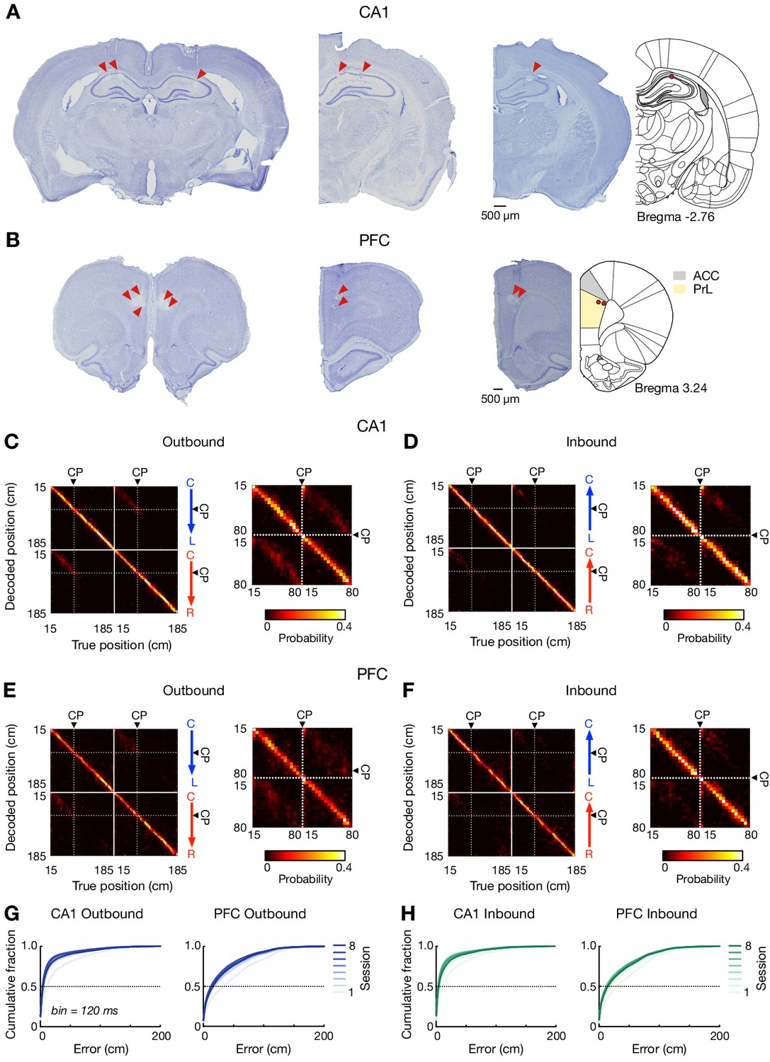
Recording locations and behavioral-sequence representations of locations over learning.
(A and B) Representative Nissl-stained coronal sections showing tetrode positions in (A) CA1 and (B) PFC (primarily in PreLimbic, PrL, cortex). Lesion locations at the end of a tetrode track are indicated by red arrowheads. Left: sections from one animal with 64 tetrodes targeting the bilateral CA1 of dorsal hippocampus and PFC. Middle and Right: sections from animals with 32 tetrodes implanted over the right hemisphere. The brain sections on the right are mapped onto a stereotaxic atlas (Paxinos and Watson, 2004) (the distance from Bregma in mm denoted). (C–F) Confusion matrices depicting actual (x-axis) and decoded (y-axis) positions in (C and D) CA1 and (E and F) PFC. For each plot pair, decoding along entire trajectories is shown on the left, and the decoding within the center stem is enlarged on the right. CP: choice point. (G and H) Cumulative position decoding errors (bin = 120 ms) across all sessions for (G) outbound and (H) inbound. Each line represents a single session (color coded). Locations within 15 cm of the reward well were excluded to prevent contamination from SWR activity. Overall decoding errors: CA1 outbound, 6.00 ± 0.08 cm; CA1 inbound, 6.00 ± 0.07 cm; PFC outbound, 18.00 ± 0.10 cm; PFC inbound, 16.00 ± 0.09 cm (median ± SEM).
Figure 2 with 2 supplements
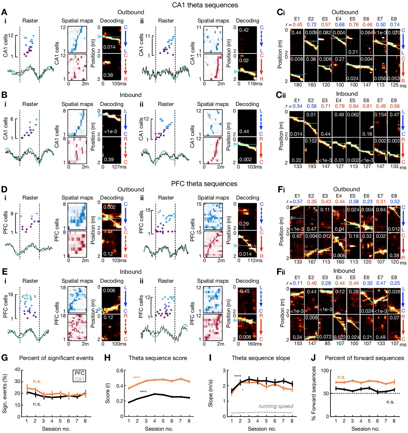
Theta sequences in CA1 and PFC over learning.
(A and B) Four examples of theta sequences in CA1 for (A) outbound and (B) inbound trajectories. Left: spikes ordered and color coded by spatial-map center on the decoded trajectory (see Right) over a theta cycle. Broadband (black) and theta-band filtered (green) LFPs from CA1 reference tetrode shown below. Middle: corresponding linearized spatial firing rate maps (blue colormap for L-side trajectory, red colormap for R-side trajectory). Right: Bayesian decoding with p-values based on shuffled data denoted (see Materials and methods). Yellow lines: the best linear fit on the decoded trajectory. Cyan lines and arrowheads: actual position. Note that summed probability of each column across two trajectory types is 1. (C) Example CA1 theta sequences across eight sessions (or epochs, E1 to E8). Each column of plots represents a theta-sequence event. Sequence score (r) on the decoded trajectory denoted. (D and E) Four examples of theta sequences in PFC for (D) outbound and (E) inbound trajectories. Data are presented as in (A) and (B). LFPs are from CA1 reference tetrode. (F) Example PFC theta sequences across eight sessions. Data are presented as in (C). (G) Percent of significant theta sequences out of all candidate sequences didn’t change significantly over sessions (Session 1 vs. 8: p’s > 0.99 for CA1 and PFC, Friedman tests with Dunn’s post hoc). Data are presented as mean and SEM. Black line: PFC; Orange line: CA1. (H) Theta sequence scores (r) improved over sessions (****p’s < 1e-4 for CA1 and PFC, Kruskal-Wallis tests with Dunn’s post hoc). Data are presented as median and SEM. (I) Theta sequence slopes increased over sessions (*p=0.0427 for CA1, and ****p<1e-4 for PFC, Kruskal-Wallis tests with Dunn’s post hoc). Dashed gray lines: mean ± SEMs of animals’ running speed (small error bars may not be discernable). Data are presented as median and SEM. (J) Percent of forward theta sequences didn’t change significantly over sessions (p=0.56 and 0.41 for CA1 and PFC, Friedman tests). Data are presented as mean and SEM.
-
Figure 2—source data 1
Percent of significant theta sequences, sequence score, sequence slope, and percent of forward theta sequences.
- https://cdn.elifesciences.org/articles/66227/elife-66227-fig2-data1-v2.xlsx
Figure 2—figure supplement 1
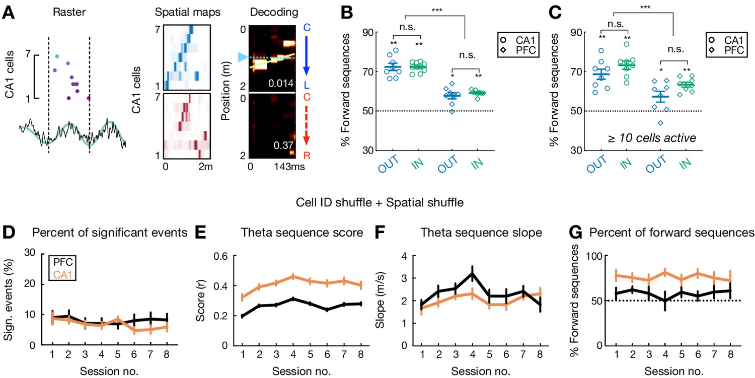
Detection of theta sequences in CA1 and PFC is statistically robust.
(A) An example of reverse theta sequences in CA1. Data are presented as in Figure 2A. (B) Percent of forward theta sequences during outbound (OUT; blue) and inbound (IN; green) running. Consistent with previous reports in CA1 (Drieu et al., 2018; Gupta et al., 2012; Wikenheiser and Redish, 2015; Zheng et al., 2016), theta sequences in CA1 and PFC are overall biased toward a forward order (**p=0.0078, *p=0.0156, signed-rank tests compared to 50%), and this bias is stronger in CA1 than PFC (***p=0.0002, Friedman test with Dunn’s post hoc). Each symbol represents a session, summing over all nine animals. Error bars: mean ± SEM. (C) Percent of forward theta sequences using a more stringent criterion of at least 10 cells active per theta cycle. Data are presented as in (B). Note that similar proportions of forward versus reverse sequences were detected independent of the cell thresholds (compared with B). (D–G) Significant theta sequences are detected in both CA1 (orange lines) and PFC (black lines) by applying additional criteria for significance in additional to the spatial shuffle (a shuffle post the Bayesian decoding; see Materials and methods). With an additional cell-identity shuffle (a shuffle prior to the Bayesian decoding), a significant theta sequence would additionally belong to the top 95th percentile of the shuffled distribution of goodness-of-fits (Rmax), and exceed the 97.5th percentile or be below the 2.5th percentile (for reverse sequences) of the shuffled distribution of weighted correlations. (D) Approximately 50% of all theta sequences in both CA1 and PFC (defined by spatial shuffles alone, therefore ~10% overall) met these additional stringent criteria, and the proportions are similar in CA1 and PFC (p=0.11, session-by-session rank-sum paired tests) regardless of the shuffling methods (compared with Figure 2G). (E) Theta sequence score, (F) Theta sequences slope, and (G) Percent of forward theta sequences with the additional criteria for significance. Data are presented as in Figure 2G–J.
Figure 2—figure supplement 2
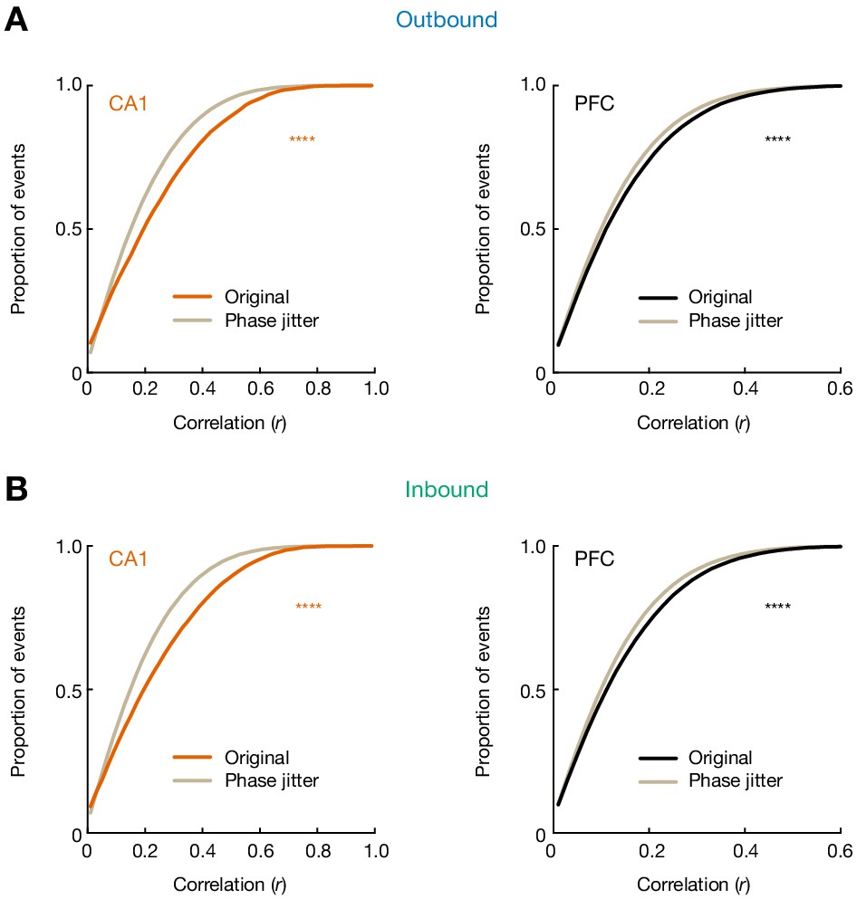
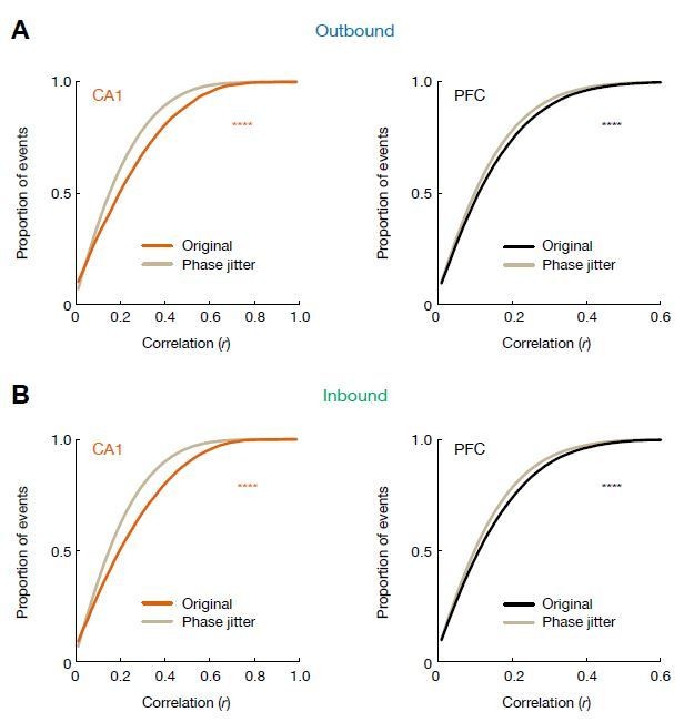
Theta phase precession does not account for the full extent of observed theta sequences in CA1 and PFC.
Cumulative distributions of theta sequence scores (or correlations, r) for original and phase-jittered events are shown. Within each candidate event, for each spike, the actual phase of that spike was randomly replaced by a phase from the distribution of possible phases associated with that cell in that position bin (without replacement, n = 100 times; Foster and Wilson, 2007). This phase-jittering shuffle thus altered the correlation between cell and time for each event. (A) Distributions for events during outbound navigation (****p=3.72e-96, and 1.28e-39 for CA1 and PFC, respectively, Kolmogorov-Smirnov tests). (B) Distributions for events during inbound navigation (****p=2.39e-132, and 4.29e-59 for CA1 and PFC, respectively, Kolmogorov-Smirnov tests). Gray lines: phase-jittered events for a given brain region. Orange line: original CA1 events. Black lines: original PFC events.
Figure 3 with 1 supplement
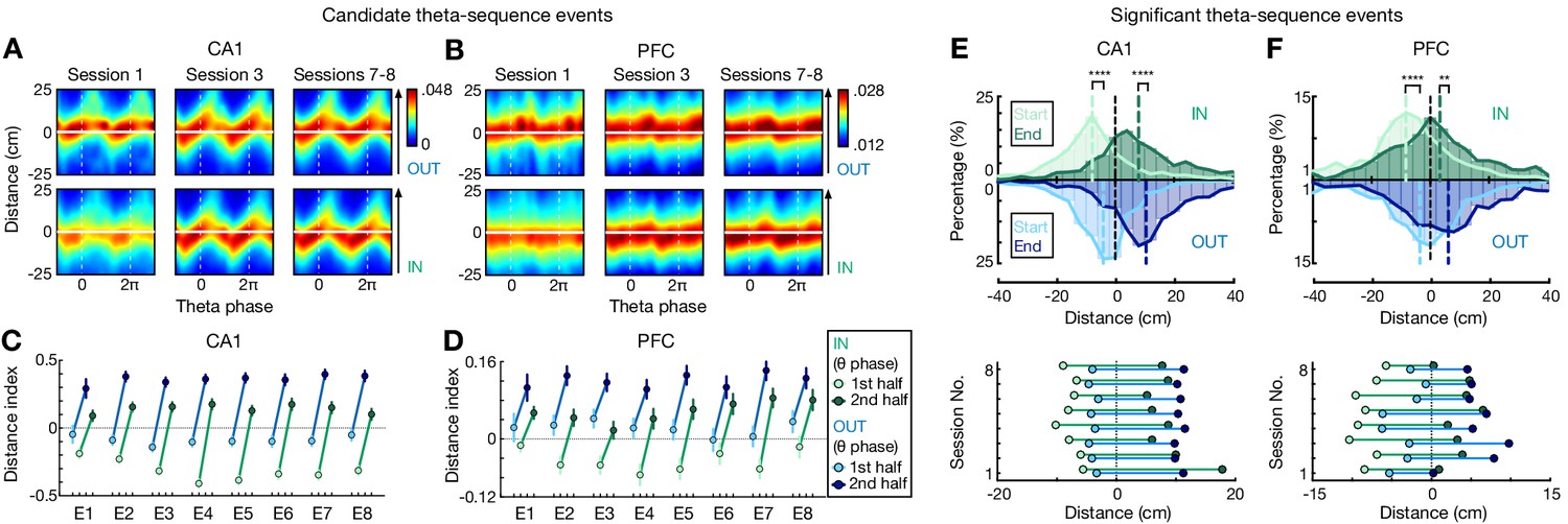
Look-ahead of CA1 and PFC theta sequences differs during outbound versus inbound navigation.
(A and B) Theta sequences representing past, current, and future locations on outbound (OUT) and inbound (IN) trajectories in (A) CA1 and (B) PFC. Each plot shows the averaged Bayesian reconstruction of all forward candidate theta sequences (sequence score r > 0), replicated over two theta cycles for visualization, relative to current position (y = 0; y > 0: ahead, or future location; y < 0: behind, or past location). Color bar: posterior probability. Arrowheaded line: animal’s running direction. (C and D) Distance index in (C) CA1 and (D) PFC across eight sessions (E1–E8), compared the posterior probabilities on future versus past locations (<0, biased to past; >0, biased to future). 1st half of theta phases (light circles): -π to 0; 2nd half of theta phases (dark circles): 0 to π. Error bars: 95% CIs. (E and F) Distributions for start and end of reconstructed trajectories relative to actual position (x = 0) of all significant forward theta sequences in (E) CA1 and (F) PFC. Top: Histograms show the distributions across all eight sessions (dashed vertical lines: median values). Bottom: Averaged trajectory start (light circles) and end (dark circles) positions in individual sessions. ****p<1e-4, **p=0.007, Kolmogorov-Smirnov test.
-
Figure 3—source data 1
Start and end of reconstructed trajectories of all significant theta sequences.
- https://cdn.elifesciences.org/articles/66227/elife-66227-fig3-data1-v2.xlsx
Figure 3—figure supplement 1
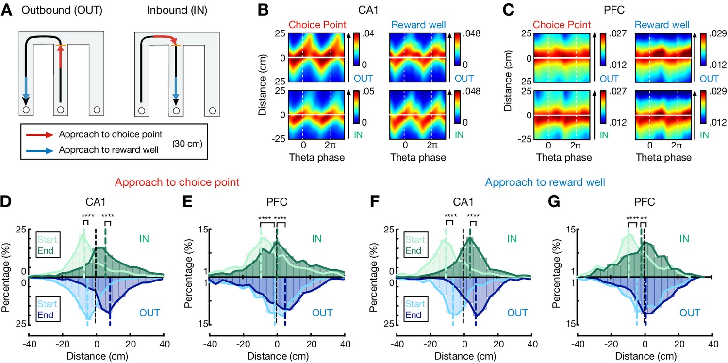
Look-ahead of theta sequences was similar during approach to choice point and approach to reward well.
(A) Schematics showing trajectory segments used for approach to choice point (red) and approach to reward well (blue) during outbound (left) and inbound (right) passes. The trajectory segment used for approach to choice point was defined as the segment 30 cm before reaching the choice point, and the trajectory segment used for approach to reward well was defined as the one 30 cm before reaching the reward-well location (i.e. 45–15 cm relative to the reward well, as the locations within 15 cm of the reward well were excluded to prevent contamination from SWR activity). (B and C) Averaged Bayesian reconstruction of all forward candidate theta sequences in (B) CA1 and (C) PFC for approach to choice point (left) versus reward well (right). Data are presented as in Figure 3A and B. (D and E) Distributions for start and end of reconstructed trajectories of all significant forward theta sequences in (D) CA1 and (E) PFC during approach to choice point. Data are presented as in Figure 3C and D. ****p<1e-4, Kolmogorov-Smirnov test. (F and G) Distributions for start and end of reconstructed trajectories of all significant forward theta sequences in (F) CA1 and (G) PFC during approach to reward well. Data are presented as in Figure 3C and D. ****p<1e-4, **p=0.0044, Kolmogorov-Smirnov test. Note that similar look-ahead properties of theta sequences were observed for approach to choice point versus reward well.
Figure 4
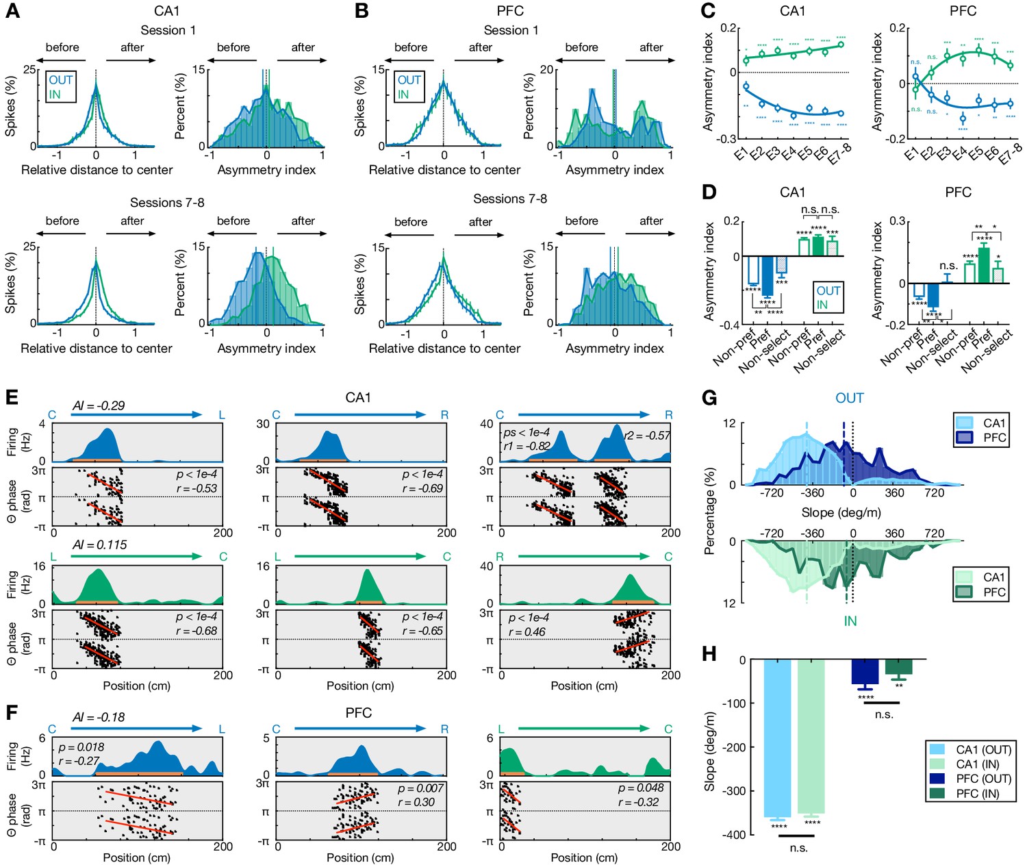
Comparisons of spatial-field asymmetry and theta phase precession during outbound versus inbound navigation in CA1 and PFC.
(A and B) Spatial-field asymmetry during Session 1 (top) and Sessions 7–8 (bottom) in (A) CA1 and (B) PFC. Blue: outbound fields (OUT); Green: inbound fields (IN). Left: Averaged firing rate relative to field center (x = 0) across all cells in the given sessions (error bars: SEMs). Right: Distributions of spatial-field asymmetry index (colored vertical lines: mean values). See also single-field examples in (E) and (F). (C) Spatial-field asymmetry index across sessions (****p<1e-4, ***p<0.001, **p<0.01, *p<0.05, n.s. p>0.05, signed-rank tests compared to 0). Lines are derived from polynomial fits. (D) Trajectory-selective cells exhibit highly asymmetric fields on the preferred (Pref) trajectory compared to the non-preferred trajectory (Non-pref). Non-select: non-selective cells. P-values for each condition derived from signed-rank tests compared to 0; p-values across conditions derived from rank-sum tests (****p<1e-4, ***p<0.001, **p<0.01, *p<0.05, n.s. p>0.05). (E and F) Single-cell examples of theta phase precession in (E) CA1 and (F) PFC for outbound (blue) and inbound (green) trajectories. For each example, linearized firing fields are shown on the top (trajectory type denoted above); spike theta phases against positions (i.e. phase precession) within individual spatial fields (indicated by an orange bar on the firing-field plot) are shown on the bottom (phases are plotted twice for better visibility; red lines represent linear-circular regression lines; linear-circular correlation coefficient r and its p-value denoted). AI: spatial-field asymmetry index. (G) Distributions of phase precession slopes for outbound and inbound fields. Top: outbound; bottom: inbound. Vertical lines: median values. (H) Phase precession slopes were similar during outbound versus inbound navigation in CA1 and PFC (n.s., p’s > 0.99, Kruskal-Wallis test with Dunn’s post hoc), and biased toward negative values (****p<1e-4, **p=0.0012, signed-rank tests compared to 0). This bias is stronger in CA1 than PFC (p’s < 1e-4, Kruskal-Wallis test with Dunn’s post hoc). Only fields with significant phase precession (see Materials and methods) are shown (mean ± SEM = 46.0 ± 2.8% in CA1, 11.2 ± 1.7% in PFC for inbound, and 48.8 ± 3.3% in CA1, 10.3 ± 1.2% in PFC for outbound). Error bars: SEMs.
-
Figure 4—source data 1
Asymmetry index and phase-precession slope.
- https://cdn.elifesciences.org/articles/66227/elife-66227-fig4-data1-v2.xlsx
Figure 5
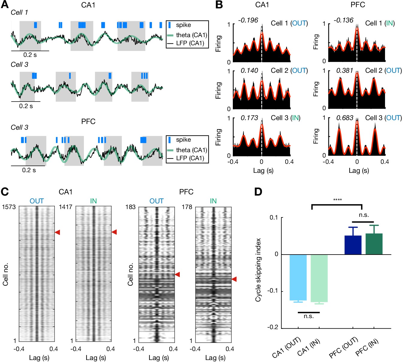
Theta cycle skipping in CA1 and PFC.
(A) Spike rasters of example cells during CA1 theta oscillations. Top: a non-skipping (firing on adjacent cycles) CA1 cell; Middle: a cycle-skipping (firing on every other cycles) CA1 cell; Bottom: a cycle-skipping PFC cell. Black and green lines: broadband and theta-filtered LFPs from CA1 reference tetrode, respectively. (B) Auto-correlograms (ACGs) of three example single cells in CA1 (left) and PFC (right). Each plot is of data from a single type of maze travel (outbound or inbound; travel type denoted). For each plot, cycle skipping index (CSI) is denoted on the upper left corner (CSI < 0: firing on adjacent cycles; CSI > 0: cycle skipping), and cell number with maze travel type (IN or OUT) matched to (A) is denoted on the upper right corner. Red line: low-passed (1–10 Hz) ACG to measure CSI (see Materials and methods). Note that cells on the bottom two rows exhibit cycle skipping, with CSI > 0. (C) ACGs of all theta-modulated cells in CA1 (left) and PFC (right) ordered by their CSIs (high to low from top to bottom). Red arrowheads indicate division between cells with CSI > 0 (above) vs. <0 (below). Each row represents a single cell with one type of maze pass (outbound or inbound). Only cells with theta-modulated ACGs are shown (see Materials and methods). Note that the proportion of theta-cycle skipping cells in CA1 is consistent with that reported in previous studies (Kay et al., 2020). (D) CSI of theta-modulated cells didn’t differ significantly on outbound versus inbound trajectories for each region (n.s., p’s > 0.99 for CA1 and PFC), but was larger in PFC than CA1 (****p<1e-4, Kruskal-Wallis tests with Dunn’s post hoc). Data are presented as mean and SEMs.
-
Figure 5—source data 1
Cycle skipping index.
- https://cdn.elifesciences.org/articles/66227/elife-66227-fig5-data1-v2.xlsx
Figure 6 with 2 supplements
Theta-sequence representations of behavioral choices in CA1 and PFC.
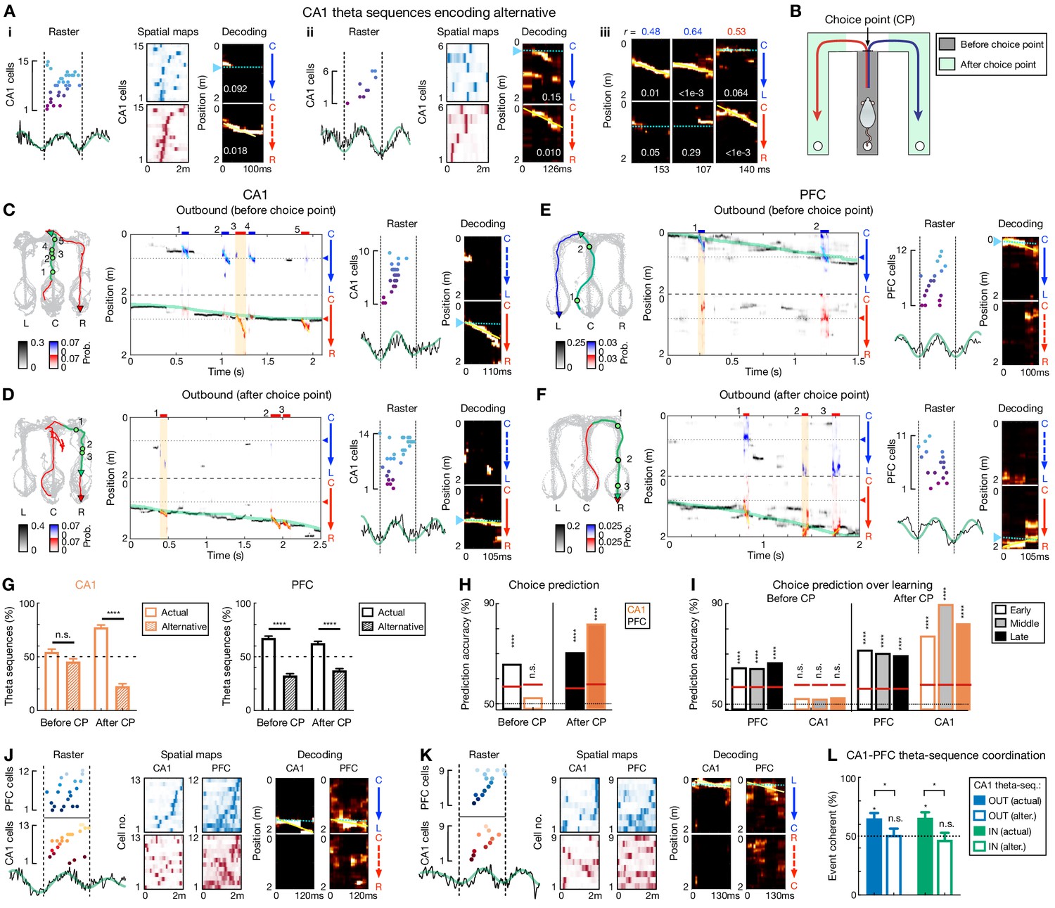
(A) Single-event examples of CA1 theta sequences encoding alternative. Two detailed example sequences are shown in (Ai) and (Aii) (presented as in Figure 2A). Three more examples with decoding plots only are shown in (Aiii) (presented as in Figure 2C). (B) Diagram showing two task segments of a behavioral trial (or trajectory): before choice point (gray shading), and after choice point (green shadings). (C–F) Four decoding examples for before and after choice point during outbound navigation in (C and D) CA1 and (E and F) PFC. Left: Animal’s behavior. Green line: the trajectory pass shown on the middle; Blue/red arrowheaded line: currently taken trajectory. Green circles: locations where theta-sequence events occurred (numbered corresponding to middle). Middle: Decoding plots. Data are presented as in Figure 1F and G (bin = 120 ms), except that whenever a theta sequence was detected, the decoding was performed on the theta timescale (bin = 30 ms) and color-coded by trajectory type for clarity (red or blue: R-side or L-side trajectory; bars above show decoded identity and timing of each event). Note that at both timescales, summed probability of each column across two trajectory types is 1. Yellow shading: example event with detailed view shown on the right. Prob.: probability. (G) Percent of theta sequences representing actual or alternative choice before and after choice point (CP) in CA1 (left) and PFC (right) (****p<1e-4, n.s. p>0.05, session-by-session rank-sum paired tests). Error bars: SEMs. (H) Trial-by-trial theta-sequence prediction of choice (****p<0.0001, n.s., p>0.05, trial-label permutation tests). Red horizontal lines: chance levels (i.e. 95% CIs of shuffled data) calculated by permutation tests. CP: choice point. (I) Theta-sequence prediction persists over sessions. Early: Sessions 1–3; Middle: Sessions 4–5; Late: Sessions 6–8. Data are presented as in (H). Only correct trials are shown in (H) and (I). CP: choice point. (J–L) Coherent CA1-PFC theta sequences biased to actual choice. (J and K) Two examples of coherent CA1-PFC theta sequences. (L) Percent of coordinated CA1-PFC theta sequences coherently representing actual vs. alternative choices (for each condition from left to right: p=0.0312, 0.94, 0.0312, 0.48, signed-rank test compared to 50%; for comparisons between two conditions from left to right, p=0.0312 and 0.0469, rank-sum tests). OUT: outbound; IN: inbound. Alter.: alternative choice. Error bars: SEMs.
-
Figure 6—source data 1
Choice representation of theta sequences, and number of coordinated theta sequences for each session.
- https://cdn.elifesciences.org/articles/66227/elife-66227-fig6-data1-v2.xlsx
Figure 6—figure supplement 1

Additional examples of theta-sequence representations of behavioral choices.
(A–F) Six additional decoding examples in CA1. (A and B) for outbound navigation. (C–F) for inbound navigation. (G–I) Three additional decoding examples in PFC. (G) for outbound navigation. (H and I) for inbound navigation. Data are presented as in Figure 6C–F.
Figure 6—figure supplement 2

Theta-sequence coding for behavioral choices during inbound navigation and additional controls.
(A) Percent of theta sequences representing current actual or alternative choice before (left two bars) and after choice point (CP; right two bars) during outbound navigation with the two shuffling procedures shown in Figure 2—figure supplement 1 (****p<1e-4, *p<0.05, n.s. p>0.05, session-by-session rank-sum paired tests). (B) Percent of theta sequences representing current actual or alternative choice before and after choice point (CP) during inbound navigation (****p<1e-4, n.s. p>0.05, session-by-session rank-sum paired tests). Similar to that during outbound navigation (Figure 6G), during inbound navigation, CA1 theta sequences encoded two possible past choices on the center stem (i.e. before CP; p=0.0934, rank-sum test compared to 50%), whereas PFC theta sequences preferentially encoded the actual choice (p<1e-4). (C) Trial-by-trial theta-sequence prediction of behavioral choice during inbound navigation. Left: During inbound navigation on the center stem, the content of CA1 theta sequences did not reliably predict animal’s current choice (n.s., p=0.473, trial-label permutation tests), but the content of PFC theta sequences predicted choice well above chance (****p<0.0001). Data are presented as in Figure 6H. Right: Theta-sequence prediction of behavioral choice persists over sessions during inbound navigation (****p<0.0001, ***p<0.001, n.s, p>0.05, trial-label permutation tests). Data are presented as in Figure 6I. CP: choice point. (D) Choice representations by the last theta sequence before choice point (CP) during outbound (OUT) and inbound (IN) navigation. The last sequence before CP of each trial was taken from the last event before exiting center stem (defined by CP) during outbound running (Figure 1A, right) and the first event after entering center stem during inbound running (Figure 1A, left). The proportions of the last sequences representing actual choices for each session are shown as mean and SEM. Solid bars are for outbound (OUT), and hollow bars are for inbound (IN). Note that the content of the last theta sequence in CA1 represented animal’s current and alternative choice equivalently (orange bars; p=0.18 and 0.13 for outbound and inbound, respectively), whereas the last theta sequence in PFC preferentially represented the actual choice (black bars; p’s < 1e-4 for outbound and inbound, signed-rank test compared to 50%).
Figure 7 with 2 supplements
Choice representations of replay sequences, but not behavioral and theta sequences, were altered in CA1 and PFC during incorrect trials.
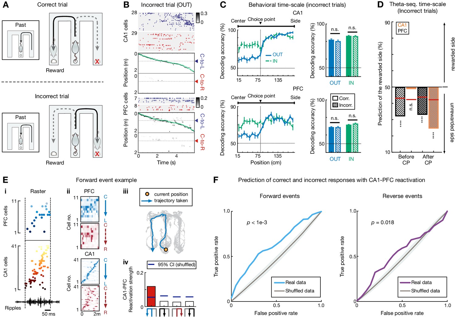
(A) Illustration of a set of correct (top) and incorrect (bottom) trials. For incorrect trial, the actual choice is the unrewarded side. (B and C) Behavioral sequences encoded current choice during incorrect trials. (B) Rasters and population decoding during an incorrect outbound trial. Data are taken from the same session and animal and presented as in Figure 1F. (C) Choice decoding accuracy during incorrect trials is not significantly different from that during correct trials in CA1 (n.s., p>0.99 for outbound,=0.67 for inbound) and PFC (n.s., p>0.99 for outbound,=0.11 for inbound; Friedman tests with Dunn’s post hoc). Corr.: correct trials; Incorr.: incorrect trials. Inbound trials for the incorrect condition were taken from the one right before an incorrect outbound trial (i.e. ‘Past’ trial of the diagram shown in A). (D) Choice representations of theta sequences were similar during incorrect and correct (see Figure 6H) trials. Black bars are for PFC theta sequences, orange bars are for CA1. CP: choice point. (E) Example forward CA1-PFC replay sequences representing actual future choice (see also Figure 1C for this event with example cells, and ripples from a different tetrode). (Ei) Ordered raster plot during a SWR event (black line: ripple-band filtered LFPs from one CA1 tetrode). (Eii) Corresponding spatial firing rate maps. (Eiii) Actual (immediate future) trajectory (orange circle: current position when replay sequences occurred). (Eiv) Reactivation strength (trajectory schematics on the bottom). Blue horizontal lines: 95% CIs computed from shuffled data. Red bar: the decoded trajectory. See Figure 7—figure supplement 2C for an example of reverse CA1-PFC replay sequences. (F) CA1-PFC replay strength predicts correct and incorrect responses. Left: Prediction using replay strength of CA1-PFC forward events. Right: Prediction using replay strength of CA1-PFC reverse events. ROC curves were computed for the SVM classifiers (p-value from trial-label shuffling denoted; see Materials and methods). Shadings: SDs.
-
Figure 7—source data 1
Decoding accuracy at the behavioral timescale for correct versus incorrect trials.
- https://cdn.elifesciences.org/articles/66227/elife-66227-fig7-data1-v2.xlsx
Figure 7—figure supplement 1
Speed, theta power, coherence, and phase-locking during correct versus incorrect outbound trials.
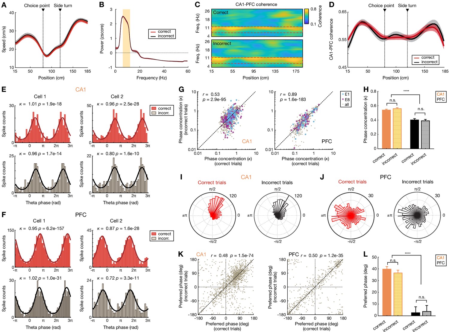
(A) Animal’s running speed during correct (red) versus incorrect (black) trials. Running speed was not significantly different across locations during correct versus incorrect trials (all p’s > 0.05, rank-sum tests). Data are presented as mean and SEM. (B) Power spectra during correct (red) versus incorrect (black) trials. Orange shading highlights the theta frequency range (6–12 Hz). Theta power was not significantly different during correct versus incorrect trials (p=0.79, rank-sum tests). Data are presented as mean and SD (small error bars may not be discernable in some cases). (C) Averaged CA1-PFC coherograms during correct (top) and incorrect (bottom) trials of an example animal in a given session. Red boxes highlight the theta frequency range. (D) CA1-PFC theta coherence was not significant different across locations during correct versus incorrect trials (all p’s > 0.05, rank-sum tests). Data are presented as mean and SEM. (E and F) Examples of phase locking to hippocampal theta oscillations for (E) two CA1 and (F) two PFC cells during correct (top) and incorrect (bottom) outbound trials. For each cell, spikes during all correct and incorrect trials of an example session are shown. Lines on the histograms are derived from von Mises fits (Jadhav et al., 2016; Siapas et al., 2005). Phase concentration parameter (κ) and p-value from Rayleigh tests are denoted. Note that while there were often fewer incorrect trials than correct trials within a given session (yielding lower spike counts for the incorrect condition), the phase-locking properties of a given cell are similar during correct versus incorrect trials. (G) Phase concentration (κ) of all significantly phase-locked cells in CA1 (left) and PFC (right) during correct versus incorrect trials. Each dot represents a single cell in a given session. Blue and purple circles highlight phase concentration during the first (E1) and last (E8) sessions, respectively. Note that phase concentration is highly correlated during correct versus incorrect trials (r- and p-values denoted on the upper left corner of each plot, Pearson correlation). (H) While CA1 population exhibited more concentrated phase distributions than PFC cells (****p<1e-4, Kruskal-Wallis tests with Dunn’s post hoc), consistent with previous reports (Jadhav et al., 2016; Siapas et al., 2005), phase concentration (κ) in each region is similar during correct versus incorrect trials (n.s., p>0.99, Kruskal-Wallis tests with Dunn’s post hoc). (I and J) Polar plots of the distributions of preferred phases of all significantly phase-locked cells in (I) CA1 and (J) PFC during correct versus incorrect trials. The preferred phase of each cell was calculated from von Mises fits. Numbers on top right indicate radius of the plot (i.e. number of neurons). Note that CA1 cells preferred the falling phase of theta, while PFC cells were most often phase locked to the trough of theta, consistent with previous studies (Jadhav et al., 2016; Jones and Wilson, 2005b; Siapas et al., 2005). (K) Preferred phase during correct versus incorrect trials in CA1 (left) and PFC (right). Each dot represents a single cell in a given session. Preferred phase is highly correlated during correct versus incorrect trials (r- and p-values denoted on the top of each plot, Pearson correlation). (L) Distributions of preferred phase during correct versus incorrect trials (****p<1e-4, n.s., p>0.99, Kruskal-Wallis tests with Dunn’s post hoc). Error bars: SEMs.
Figure 7—figure supplement 2
CA1-PFC reactivation strength during correct versus incorrect trials.
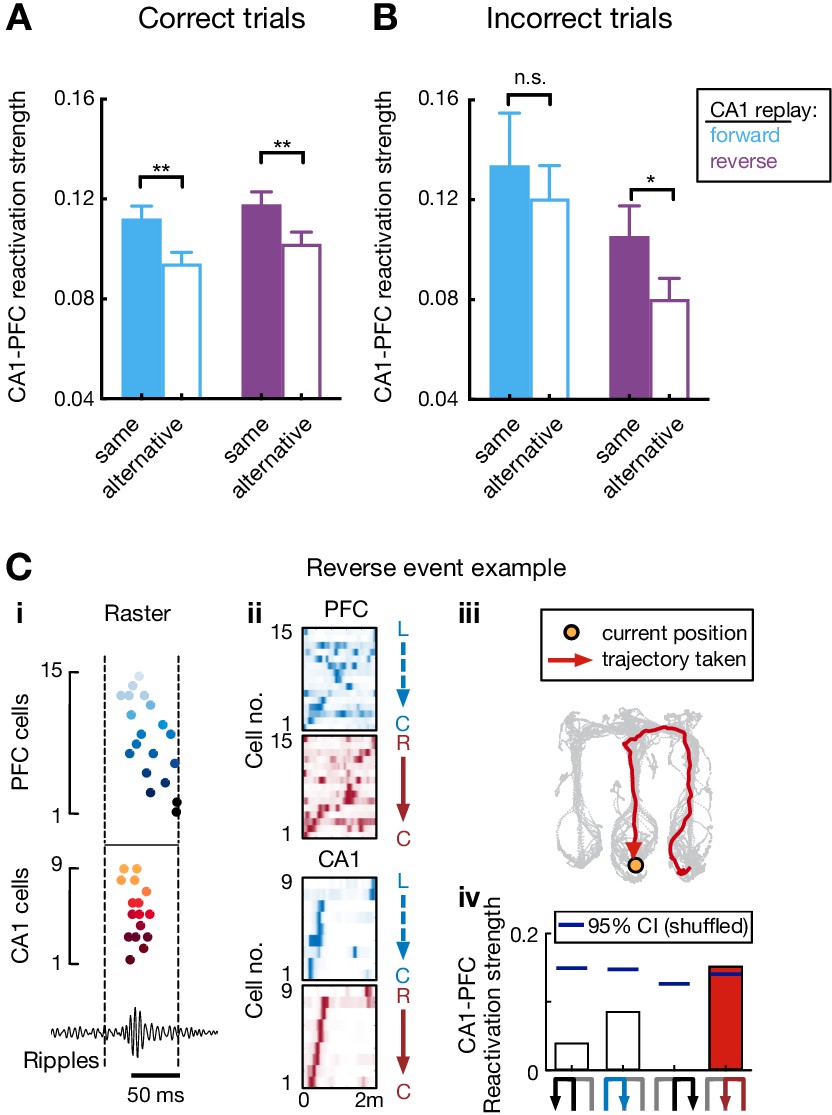
(A and B) CA1-PFC reactivation of taken path compared to not-taken path during (A) correct and (B) incorrect trials for forward and reverse CA1 replay (correct trials: **p=0.0016 and n = 351 events for forward replay of taken path; **p=0.0037 and n = 393 events for reverse replay of taken path; incorrect trials: p=0.56 and n = 38 events for forward replay of taken path; *p=0.024 and n = 48 events for reverse replay of taken path; event-by-event paired t-tests). Results were consistent with our previous report (Shin et al., 2019). The reactivation strengths of taken (actual) path and not-taken (alternative) path were used as 2D features for the SVM classifiers in Figure 7F. (C) Example reverse CA1-PFC replay sequences representing actual past choice at the center well. Data are presented as in Figure 7E.
Author response image 1

Author response image 2
Cumulative distributions of theta sequence scores (or correlations, r) for actual and phase-jittered events.
(A) Distributions for events during outbound navigation (****p = 3.72e-96, and 1.28e-39 for CA1 and PFC, respectively, KS tests). (B) Distributions for events during inbound navigation (****p = 2.39e-132, and 4.29e-59 for CA1 and PFC, respectively, KS tests). Gray lines: phase-jittered events for a given brain region. Orange line: original CA1 events. Black lines: original PFC events.
Author response image 3
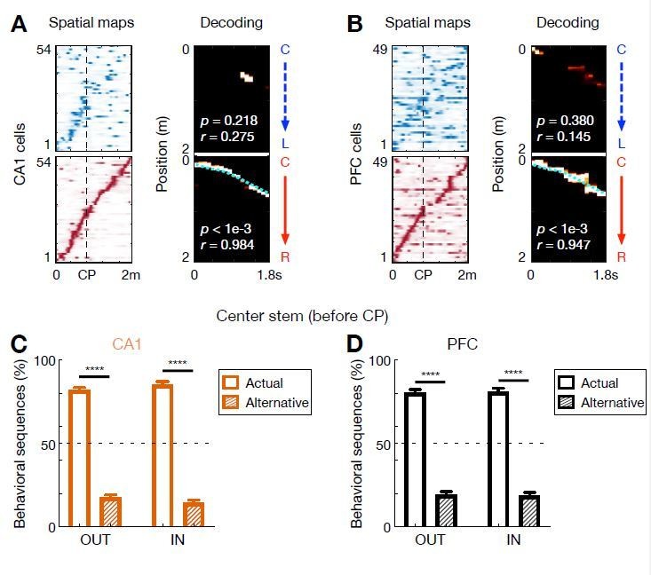
Behavioral-sequence representations of choices in CA1 and PFC.
(A and B) Single-event examples of (A) CA1 and (B) PFC behavioral sequences simultaneously recorded during a C-to-R outbound trial. Left: corresponding linearized spatial firing rate maps (blue colormap for L-side trajectory, red colormap for R-side trajectory). Right: Bayesian decoding with sequence score (r) and p-values based on shuffled data denoted. Cyan lines: actual position. Note that a few single-bin decoding errors of current choices occurred along a sequence. Also note the global remapping of some cells on different trajectory types (CP: choice point). (C and D) Percent of behavioral sequences representing actual or alternative choice before the choice point (CP) for outbound (OUT) and inbound (IN) trials in (C) CA1 and (D) PFC (****p < 1e-4, session-by-session rank-sum paired tests). Error bars: SEMs. Data are presented as in Figure 6G. The choice representation of each behavioral sequence was determined by a sequential decoder, similar to that for theta sequences.
Videos
Video 1
Slow-motion video of behavioral-timescale and theta-sequence decoding in CA1 when the rat is running a Center-to-Right outbound trajectory.
The video plays 7.5 times slower than real time. To better visualize fast theta sequences, when a significant theta sequence is detected, the video plays 15 times slower. Audio represents spiking of all example units shown on the raster (top left; each spike was correspondingly sped up 7.5 times around spike detection for better perception). Bottom left: Decoding plot. For each theta sequence, reconstruction of only the decoded trajectory was shown for clarity. Right: Behavioral video. Green circle: true position. White circle with a pair of arrowheads: estimated position decoded at the behavioral timescale (arrowhead colors indicate trajectory type, blue for L-side trajectory, red for R-side trajectory; solid arrowheads: decoded trajectory type. hollow ones: the alternative). Note that the raster only shows cells that participated in theta sequences for better visualization, whereas the decoding was performed using all place cells recorded.
Video 2
Slow-motion video of behavioral-timescale and theta-sequence decoding in CA1 when the rat is running a Right-to-Center inbound trajectory.
The video is presented as in Video 1.
Video 3
Video of CA1 replay sequences representing possible future choices.
The video is displayed in real time, but two times slower during immobility at the reward well to better visualize fast replay sequences. Top left: Raster of example CA1 cells ordered and color coded by place field center on the actual future trajectory (C-to-L). Bottom left: Raster of the same CA1 population shown on top left, but ordered and color coded by place field center on the alternative future trajectory (C-to-R). Right: Behavioral video. Green circle: true position. Large arrowhead: estimated location at the behavioral timescale. Due to the long immobility period at the reward well (9.58 s), only 1 s around each replay event detected was shown. When a replay sequence is detected, the decoded trajectory is represented by an arrowheaded line (colored according to the trajectory type, blue for L-side trajectory, red for R-side trajectory).
Tables
Key resources table
| Reagent type (species) or resource | Designation | Source or reference | Identifiers | Additional information |
|---|---|---|---|---|
| Strain, strain background (Long Evans rats; male) | Long Evans | Charles River | Cat#: Crl:LE 006 RRID: RGD_2308852 | |
| Chemical compound, drug | Cresyl Violet | Acros Organics | Cat#: AC229630050 | |
| Chemical compound, drug | Formaldehyde | Fisher | Cat#: 50-00-0,67561,7732-18-5 | |
| Chemical compound, drug | Isoflurane | Patterson Veterinary | Cat#: 07-806-3204 | |
| Chemical compound, drug | Ketamine | Patterson Veterinary | Cat#: 07-803-6637 | |
| Chemical compound, drug | Xylazine | Patterson Veterinary | Cat#: 07-808-1947 | |
| Chemical compound, drug | Atropine | Patterson Veterinary | Cat#: 07-869-6061 | |
| Chemical compound, drug | Bupivacaine | Patterson Veterinary | Cat#: 07-890-4881 | |
| Chemical compound, drug | Beuthanasia-D | Patterson Veterinary | Cat#: 07-807-3963 | |
| Software, algorithm | MATLAB 2017a | Mathworks, MA | RRID: SCR_001622, V2017a | |
| Software, algorithm | Trodes | SpikeGadgets | https://spikegadgets.com/trodes/, V1.9 | |
| Software, algorithm | Matclust | Mattias P. Karlsson | https://www.mathworks.com/matlabcentral/fileexchange/39663-matclust, V1.7 | |
| Software, algorithm | Libsvm | Chang and Lin, 2011 | RRID:SCR_010243 https://www.csie.ntu.edu.tw/~cjlin/libsvm/, V3.12 | |
| Software, algorithm | Chronux | Partha Mitra | RRID:SCR_00554 http://chronux.org/, V2.12 | |
| Software, algorithm | measure_phaseprec Toolbox | Kempter et al., 2012; Sanders et al., 2019 | https://github.com/HoniSanders/measure_phaseprec | |
| Software, algorithm | Prism 8 | GraphPad Software | RRID: SCR_002798, V8.0 |
Additional files
Download links
A two-part list of links to download the article, or parts of the article, in various formats.
Downloads (link to download the article as PDF)
Open citations (links to open the citations from this article in various online reference manager services)
Cite this article (links to download the citations from this article in formats compatible with various reference manager tools)
Multiple time-scales of decision-making in the hippocampus and prefrontal cortex
eLife 10:e66227.
https://doi.org/10.7554/eLife.66227


