Heterogeneous side effects of cortical inactivation in behaving animals
- Department of Neurobiology and Anatomy, McGovern Medical School, University of Texas, United States
- Department of Neurology, McGovern Medical School, University of Texas, United States
- Center for Membrane Biology, Department of Biochemistry and Molecular Biology, McGovern Medical School, University of Texas, United States
Figures
Figure 1 with 1 supplement

Optogenetic suppression yields heterogeneous responses in the distal network.
(A) Left, glutamatergic neurons were targeted using a lentivirus construct, containing the gene for GtACR2, under the control of an α-CamKII promoter. Right, optogenetic suppression of a focal neural population may result in a spread of suppression across the network (‘Suppression only’) or in a heterogeneous response in the network (‘Mixed effects’). (B) Immunohistochemical analysis performed on biopsied tissue from one monkey, after experiments were complete, confirmed that expression of green fluorescent protein (GFP)-tagged GtACR2 was confined exclusively to excitatory neurons. White arrowheads indicate neurons immuno-positive for NeuN (pan-neuronal marker, top left panel), α-CamKII (glutamatergic neuron marker, top right panel), and GFP (GtACR2 marker, bottom left panel). Right, bar graph shows counts for immuno-positive cells counted across five separate sections. No inhibitory neurons (NeuN+/CamKII-) were found to be positive for GFP. Scale bar is 25 μm. (C) Animals viewed 300-ms contrast-varying oriented gratings on a computer monitor. Optogenetic suppression was present on 50% of trials in a randomly interleaved manner. Light duration was 300 ms and was synchronized with stimulus presentation. (D) Electrophysiological recordings using laminar electrodes were made either proximal to the fiber optic location or at distal sites ~300 μm away. (E) Neural responses near the light source. Population responses (n = 48) with (blue trace) and without (black trace) laser activation of GtACR2, while animals fixated. Horizontal black bar shows time of light on. Error envelopes show sem. (F–I) Examples of neural responses recorded distal from the fiber optic, across four visual stimulus conditions (columns). Columns are arranged with increasing stimulus contrast (0%, leftmost column, to 100%, rightmost column). Black traces show the mean firing rate on control trials. Colored traces show mean firing rates on laser trials. Horizontal black line shows timing of the visual stimulus and light on; red arrowheads mark regions of interest.
Figure 1—figure supplement 1
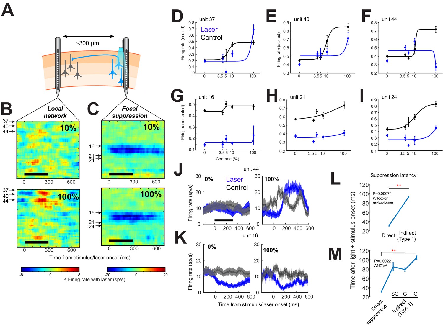
Example session with simultaneous dual recordings showing direct suppression at the illumination site and heterogeneous responses in the distal network.
(A) Schematic of the recording setup using two laminar electrodes separated by 300 µm. A fiber optic is closely coupled with one of the electrodes. (B, C) Heatmaps showing the differences in firing rates (laser minus control trials) across all simultaneously recorded channels from the distal electrode in the local network (B) and the electrode coupled to the fiber optic light source (C). Upper and lower heatmaps show response differences during stimuli of 10% and 100% contrast, respectively. Arrows with numbers show the units depicted in panels (D–I). Blue traces show results from optical suppression (‘Laser’) trials. Black traces show control trials. (D–I) Contrast response function of 3 units from the distal probe (D–F) and 3 units from the optical suppression site (G–I). Responses were calculated for the 150 ms window that evoked the strongest response on control trials, typically 0–150 ms from stimulus onset (see ‘Materials and methods’ for details). (J, K) Peri-stimulus time histograms for 2 units, one from the distal probe (J) and one from the optical suppression site (K). Left panels show average firing rates during 0% contrast trials in control (black) and optical suppression (blue) trials. Right panels show average firing rates during 100% contrast trials. Stimulus orientation was close to the preferred orientation of the distal probe population, but not optimized. All errors show sem. (L) Type 1 cells recorded 300 µm from the light source (‘indirect’; n = 91) displayed significantly longer latencies to reach maximum suppression compared to cells near the light source (‘direct’; n = 41), measured as the first time after light onset at which the maximum percent suppression during light and visual stimulation is reached. (M) Subdividing the Type 1 indirect cells across layers (n = 12, 21, and 28 for supragranular (SG), granular (G), and infragranular (IG) layers, respectively) also showed that the indirect cells had a longer response latency compared to direct cells across all layers. This strongly supports the idea that the indirect effects are mediated by local circuitry.
Figure 2 with 3 supplements
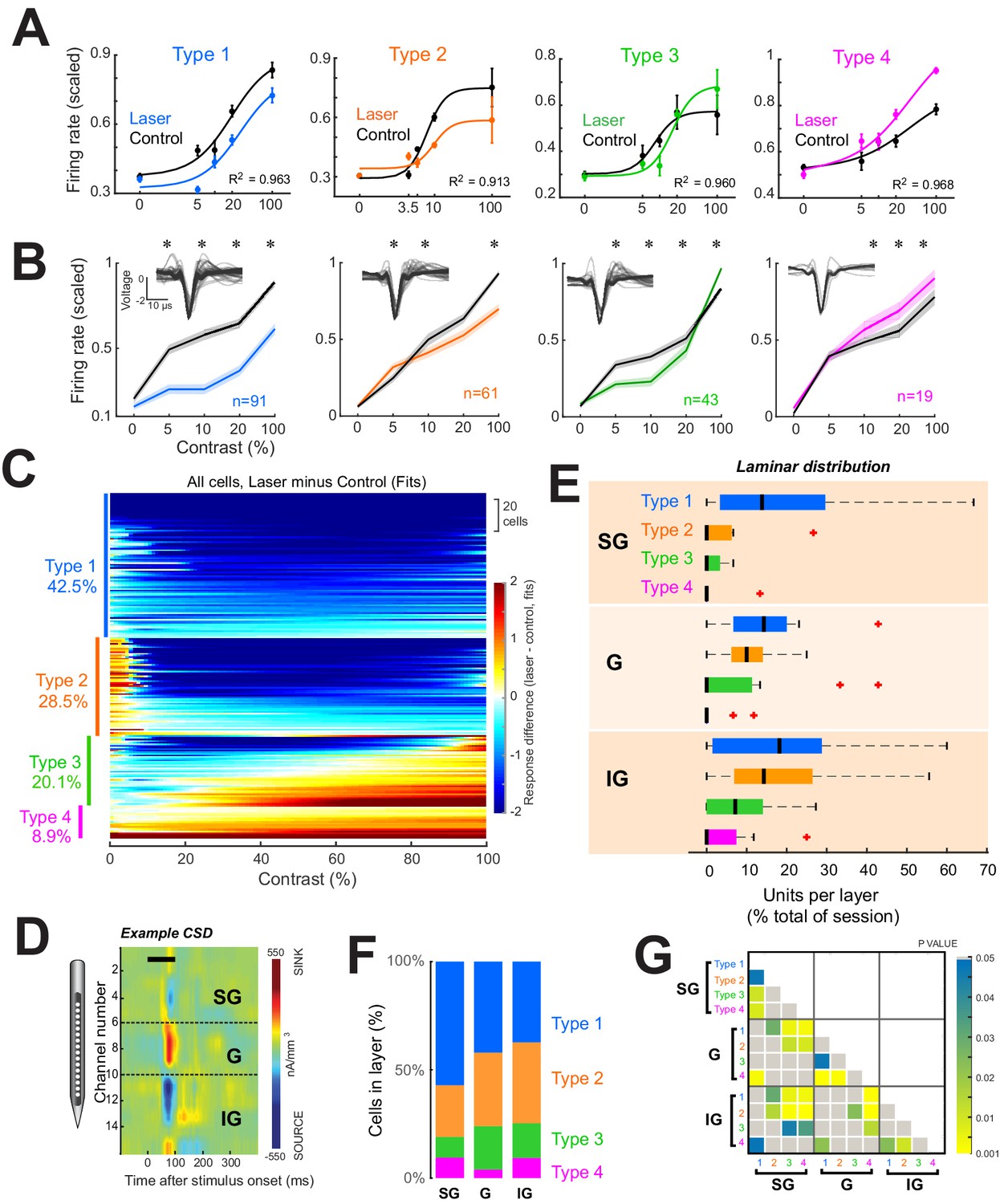
Four response motifs observed across cortical layers.
(A) Representative examples for the four distinct response patterns observed. Points show mean ± standard error of firing rates scaled relative to the maximum across trials. Solid lines show normalization model fits to data points. Black points/lines show basic responses. Colored points/lines show responses during optogenetic suppression of local network. (B) Population contrast responses for each response type. *p<0.05, Wilcoxon signed rank test, with false discovery rate correction. Insets show average waveforms from all cells. (C) Response types across the population. Heatmap shows differences in firing rate (laser minus control) as predicted by normalization fits for each recorded neuron. Types were classified based on the model fit pattern and ordered based on the mean change in firing rate between laser and control trials across contrasts. (D) Example current-sink density estimate for one session, used to assign layer identity. Black horizontal bar shows the time of stimulus presentation. Dashed horizontal black lines show layer boundaries (see ‘Materials and methods’). (E) Distributions of response types per layer as a percent of all cells recorded in each layer across all sessions. Black vertical line represents the median. Edges of boxes represent the 25th and 75th percentiles. Dashed lines represent the range. Red crosses represent outliers. Inset shows the percent of each response type within each layer. (F) Proportion of each response type within each layer. (G) Results of statistical comparisons of distributions shown in panel (E) (Kruskal-Wallis test, post-hoc Tukey test).
Figure 2—figure supplement 1
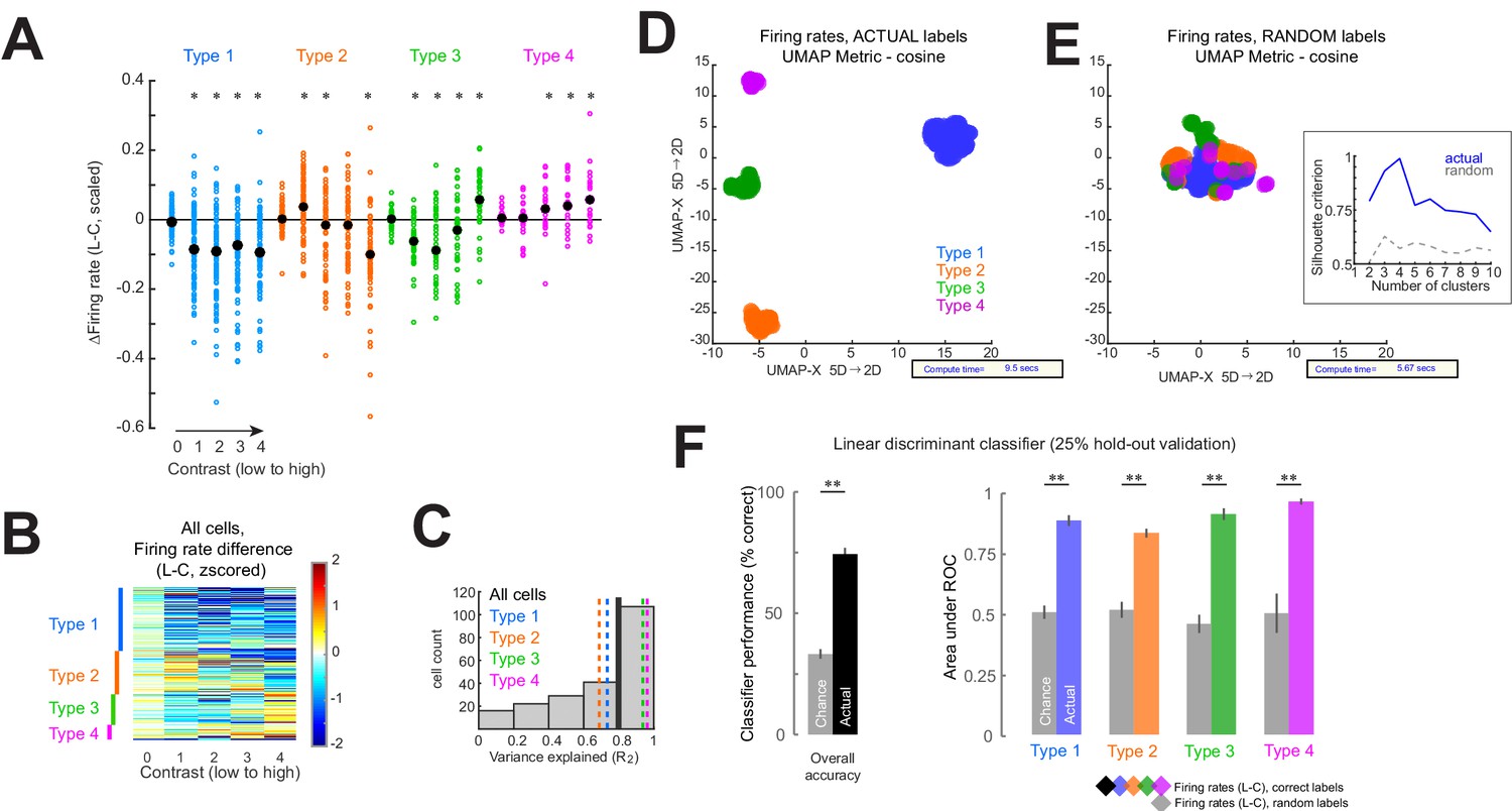
Response type classification captures firing rate differences.
(A) Change in firing rate on laser trials compared to control across contrasts for all neurons (n = 214), classified according to the normalization fits (Types 1–4; see also Figure 2). Black dots represent the mean of each distribution. *p<0.05, Wilcoxon signed rank test, median different from zero, with false discovery rate correction for multiple comparisons. (B) Actual firing rate changes for each contrast that models were fit to and ordered as in panel (B). Color scheme is identical to that in panel (B). (C) Variance explained values for model fits of the entire population of neurons. Vertical lines show the median of the entire population (black solid line) and the medians of groups divided by response types (colored dashed lines). (D, E) To validate that the response type classification procedure based on the normalization fits captured the actual firing rate changes for each cell, we used a uniform manifold approximation and projection (‘UMAP’) algorithm to cluster the firing rate differences (laser minus control) across all contrasts for all cells (n = 214). Firing rate differences across contrasts with correctly ascribed labels produce four distinct clusters (D), while randomly ascribed labels to the same firing rate data produce only one cluster (E). The number of clusters was assessed using the silhouette criterion (E, inset; highest value corresponds to the optimal number of clusters; blue line shows criterion values for K-means clustering of UMAP values obtained from the actual data, as shown in panel (D), while the gray dashed line shows criterion values for clustering based on random assigned labels, panel (E) main). This demonstrates that the clustering obtained in (D) does not arise by chance and confirms that the UMAP method, based on the actual data, produces four highly separable clusters. (F) As a secondary validation that the response type classification method we implemented a linear discriminant classifier to classify the ascribed response type based on the firing rate differences (laser minus control) across all contrasts for each cell. The overall performance of the classifier is shown on the left (black bar, mean ± sem based on five runs) and performed significantly (**p<0.0001, t-test, two-way, unpaired; n = 5 runs) above chance (gray bar, same firing rate data but with randomly shuffled class labels). The area under the receiver operating characteristic curves for each response type is significantly above chance (**p<0.0001, t-test, two-way, unpaired; n = 5 runs) for all response types (right side).
Figure 2—figure supplement 2
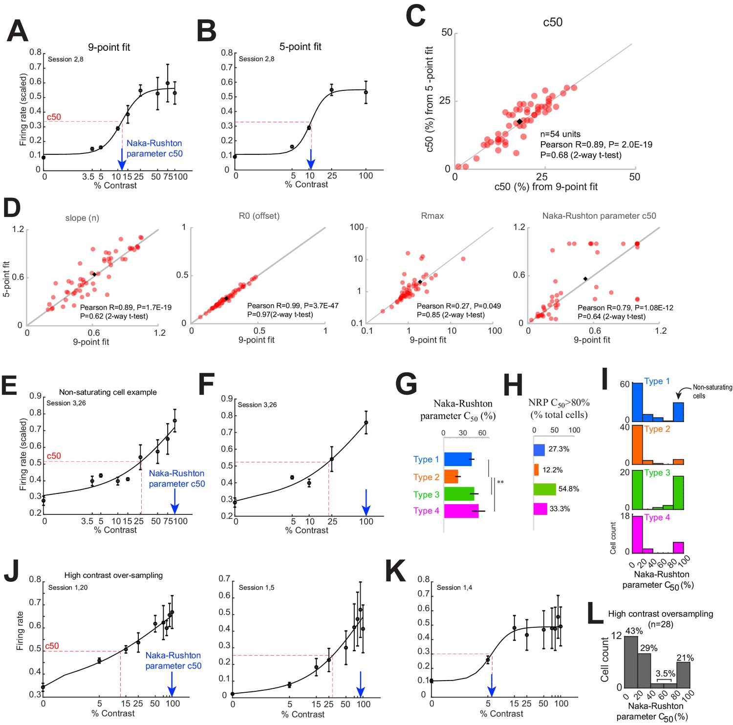
Normalization model fit parameters based on five contrasts are nearly identical to those estimated from nine contrasts.
(A) Contrast response curve from an example cell based on responses to nine visual contrasts. Dashed red line shows c50 of the fit. Blue arrow shows the c50 parameter of the normalization fit (based on Naka-Rushton equation). (B) Same cell as in panel (A), with contrast response curve fit using a subset of five contrasts. (C) c50 measured from contrast response curves fit using nine vs five contrasts. Inset details the R and p-values of the Pearson correlation, and the p-value of a two-way, paired t-test comparing the nine and five contrast groups (n = 54). (D) Comparison of other normalization fit parameters from nine vs five point fits. (E, F) Contrast response curve for an example cell that does not show response saturation at high-contrast fits with either nine (E) or five contrasts (F). For these cells, the estimated c50 parameter (blue arrow) does not correspond with the measured c50 (red dashed line). (G) Normalization c50 parameter for each response type. Bars show the mean and standard error of each group. **p<0.001, Kruskal-Wallis test, with post-hoc Tukey test. (H) Percent of cells with model parameter c50 values greater than 80% contrast, indicative of non-saturating behavior, for each response type. (I) Distribution of model parameter c50 values for each response type. (J–L) Oversampling the high-contrast range still shows cells that do not saturate at even very high contrasts. (J) Left and right panels show example cells with non-saturating behavior. (K) Example cell simultaneously recorded with those in panel (J), which exhibit more typical high-contrast saturating behavior. (L) Distribution of model parameter c50 values obtained from the high-contrast oversampling experiment. This distribution is very similar to those in panel (I), strongly suggesting that the non-saturating cells in panel (I) are a true category, rather than an artifact due to under-sampling at high contrasts.
Figure 2—figure supplement 3
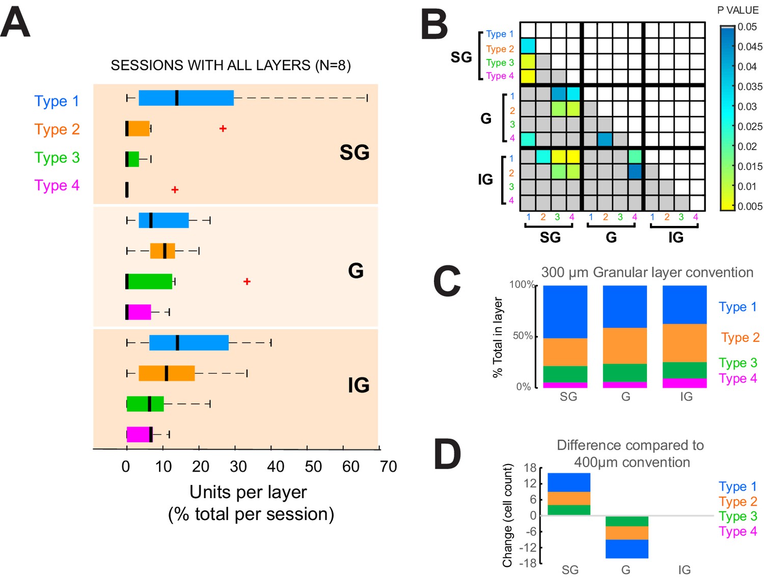
Laminar distribution of response types across sessions with all layers simultaneously recorded.
(A) Response types per layer as a percent of all cells recorded in each layer across all sessions. Black vertical line represents the median. Edges of boxes represent the 25th and 75th percentiles. Dashed lines represent the range. Red crosses represent outliers. N = 8 sessions, with 66 total units. Results are comparable to those of the complete dataset shown in Figure 3. (B) Results of statistical comparisons of distributions shown in panel (A) (Kruskal-Wallis test, post-hoc Tukey test). (C) Given the lack of clear consensus about the thickness of the granular layer in the macaque brain, we also classified layers using a smaller 300-µm granular layer convention to check whether it produced less heterogeneity across layers. The distribution of response types per layer, however, was very similar to that using the 400 µm convention (Figure 2F). (D) Reducing the granular layer thickness convention from 400 µm to 300 µm resulted in layer assignment changes (granular (G) to supragranular (SG)) for 16 cells (n = 7 Type 1, n = 5 Type 2, n = 4 Type 3, and n = 0 Type 4).
Figure 3 with 2 supplements
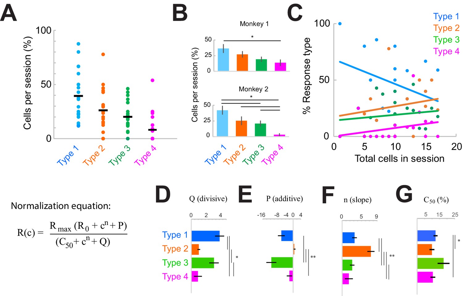
| Response type distributions are stable across sessions and subjects.
(A) Proportion of neurons in each category type recorded in each session. Horizontal black line shows the mean across sessions. (B) Proportion of neurons in each category across sessions in each monkey. *p<0.05, Kruskal-Wallis test, post-hoc Tukey test. (C) Sample-size effect. Sessions with higher overall cell counts have a greater proportion of Type 2–4 cells and fewer Type 1 cells. The y-axis represents the percent of each response type as a function of the total number of cells recorded in each session (n = 22). Lines represent linear fits of each response type. (D–F) Normalization model fit parameters for each response type, showing the divisive (D) and additive (E) components as well as the slope (F). (G) Contrast that elicits 50% of the maximum response (c50), measured from fits. Bars show the mean and standard error of each group. *p<0.05, **p<0.001, Kruskal-Wallis test, with post-hoc Tukey test.
Figure 3—figure supplement 1
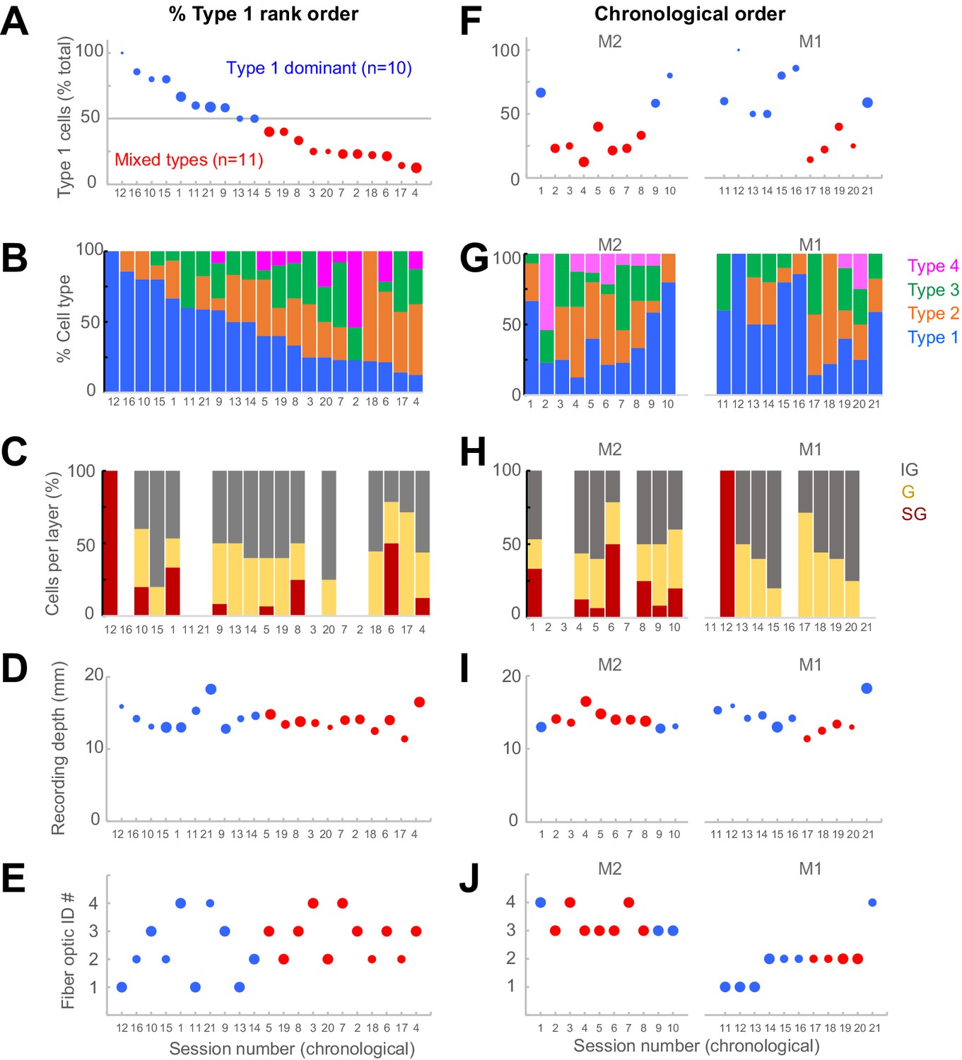
Cross-session heterogeneity not explained by known experimental factors.
We assessed whether the variations in response types across sessions could be explained by other factors. The panels in the left column have sessions ordered by the % Type 1 responses contained. The panels in the right column show the same data arranged in the chronological recording order, with a small gap indicating data from individual monkeys (‘M1’, ‘M2’). (A, F) Percent Type 1 cells of total cells recorded in each session. The size of dots is proportional to the total number of cells in each session, ranging from 1 to 17 cells. (B, G) Distribution of all response types per session. Trial counts for each session numbered 1–21 are 128, 320, 288, 192, 144, 288, 432, 480, 480, 384, 240, 288, 480, 432, 282, 244, 480, 480, 480, 240, and 480, respectively. (C, H) Distribution of cells in each layer division (supragranular (SG), granular (G), infragranular (IG)). Sessions without data did not have clear laminar information. (D, I) Relative depth of recording electrode, zeroed to a pre-defined point on the microdrive apparatus prior to mounting it on the chamber. Dot size represents the number of cells in the session, like panels (A, F). (E, J) Four different fiber optic cables were used in these experiments, identified here by numbers 1–4. Dot size is proportional to the laser power setting from the collimator to the fiber optic (numerical values of 6 or 10).
Figure 3—figure supplement 2

Orientation preference and tuning sharpness are equally variant across Type 1 dominant sessions and mixed-type sessions.
(A) Orientation preference of light-responsive neurons was assessed using a reverse-correlation fixation task presenting static gratings of eight orientations. Sessions that have no data (n = 5) did not include this additional fixation task, when time did not permit. To measure the heterogeneity of orientation tuning within individual sessions, we calculated the standard deviation of preferred orientation across all light-responsive neurons within each Type 1 dominant session (blue circles) and mixed-type session (red circles). Sessions are arranged according to the % Type 1 cells in the descending order (left panel) or the chronological recording order (right panel). (B) Standard deviation of the orientation selectivity index (OSI) across the light-responsive cells in each session. Same conventions as in panel (A). (C) Difference in orientation between each light-responsive neuron and the actual stimulus orientation was not different across response types (p = 0.725, Kruskal-Wallis test, df = 3). (D) Orientation selectivity was not different across response classes (p = 0.120, Kruskal-Wallis test, df = 3).
Figure 4 with 1 supplement
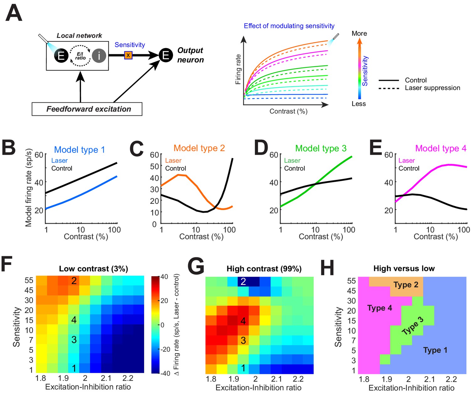
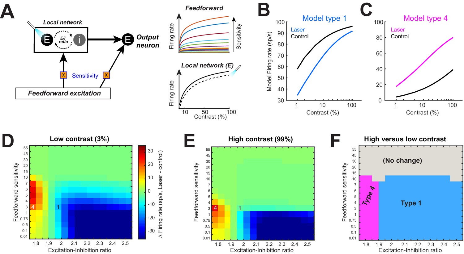
Model replicates heterogeneous responses to optical suppression of local network by altering network stimulus sensitivity.
(A) Cartoon model (left). The response of the output neuron is calculated as a linear summation of a feedforward and a local network component. Feedforward drive is purely excitatory, while the local network is represented as a mixture of excitation and inhibition currents. Inhibition followed excitation according to a fixed ratio (‘E–I ratio’). The gain of the excitatory current is modulated by a multiplicative parameter (‘sensitivity’). (Right) The firing rate of the output neuron as network sensitivity is varied. Solid colored traces show model responses on control trials. Dashed lines represent optogenetic suppression trials. (B–E) Varying the sensitivity of the network input while holding E/I ratio stable produces the four basic response motifs observed experimentally. The parameters used to generate these responses are shown in panels (F, G). (F, G) Differences in the model firing rate between laser and control trials for low-contrast (F) and high-contrast stimuli (G), while varying the local network sensitivity (y-axis) and E/I ratio (x-axis). Overlaid numbers represent the parameter combinations for generating the response types in panels (B–E). (H) Boundaries of parameter space dividing the four response types based on changes in firing rate associated with optogenetic suppression for low (H)- and high (G)-contrast conditions.
Figure 4—figure supplement 1
Modulating sensitivity of model feedforward input is insufficient to reproduce experimentally observed effects.
(A) Model neuron implementation identical to Figure 4, except that the sensitivity of the feedforward input (orange box) was varied, while the drive of the local network (normalization pool) was kept constant. The local network stimulus response was modeled as a hyperbolic ratio, with a slope, n = 0.8, an sem i-saturation constant, c50 = 25% contrast, and a baseline firing rate of 20 sp/s. Optogenetic suppression was again represented as a fixed reduction of 12.9 sp/s in the steady-state excitatory component of local network activity. (B, C) Varying the sensitivity of the feedforward input can reproduce two of the four experimentally observed response types. Parameters used to generate these responses are shown in panels (D, E). Unlike the results of varying the gain of the local network (Figure 4), simultaneous observation of both types could only occur under different excitation-inhibition regimes. (D, E) Changes in the model firing rate between laser and control trials for low-contrast stimuli (D) and high-contrast stimuli (E), while varying the feedforward input stimulus sensitivity (y-axis) and the excitation-inhibition (E-I) ratio of the local network drive (x-axis). Overlaid numbers refer to parameter combinations used to generate the response types shown in panels (B, C). (F) Division of parameter space into response types based on changes in firing rate associated with optogenetic suppression observed in low (D)- versus high (E)-contrast conditions. Black dashed line shows the minimum range of sensitivity and E-I ratio values required to be present in the entire population to simultaneously account for all four response types.
Figure 5 with 2 supplements
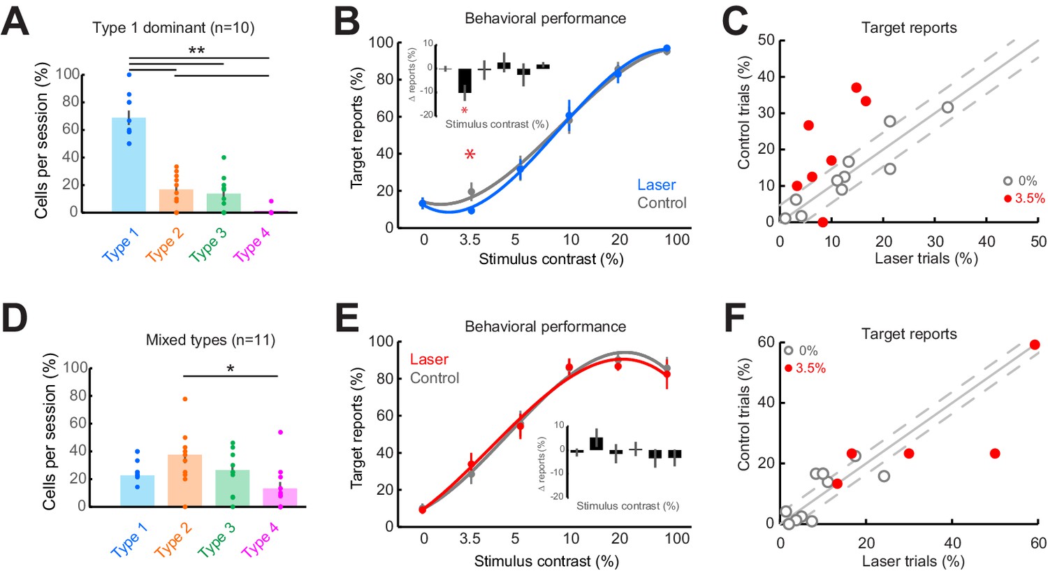
Consistent impairment in behavioral performance occurs only when optogenetic inactivation is associated with homogeneous response suppression in V1.
(A) Proportions of cell response types found in those sessions containing >50% Type 1 responses. Dots show individual sessions. Bar graphs show mean ± sem. **p = 2.30 × 10⁻⁶, one-way Kruskal-Wallis test (df = 3, Chi-sq = 28.94, post-hoc t-test). (B) Task performance in Type 1 dominant sessions showing % trials in which animals reported the presence of a visual stimulus on laser (blue) and control (gray) trials. *p = 0.04, t-test, paired, two-way. Session counts per contrast, ascending (left to right), are 10, 7, 10, 9, 3, and 8. Points show mean ± sem. Fits are third-order polynomials. Inset bar graph shows performance difference (laser minus control) across contrasts. (C) Target reports for Type 1 dominant sessions (n = 10) for 0% (open gray circles) and 3.5% (red filled circles) contrast. The unity line (solid gray diagonal) shows ± sem behavior responses across all contrasts in control condition (flanking dashed diagonal lines). (D) Same conventions as in panel (A), but for the sessions with mixed response types; *p = 0.022, one-way Kruskal-Wallis test (df = 3, Chi-sq = 9.67, post-hoc t-test). (E) Same conventions as in panel (B), showing no change in behavioral performance across laser (red) and control (gray) trials. Session counts per contrast, ascending (left to right), are 11, 5, 10, 11, 6, and 9. (F) Same conventions as in panel (C), but for mixed-type dominant sessions (n = 11).
Figure 5—figure supplement 1
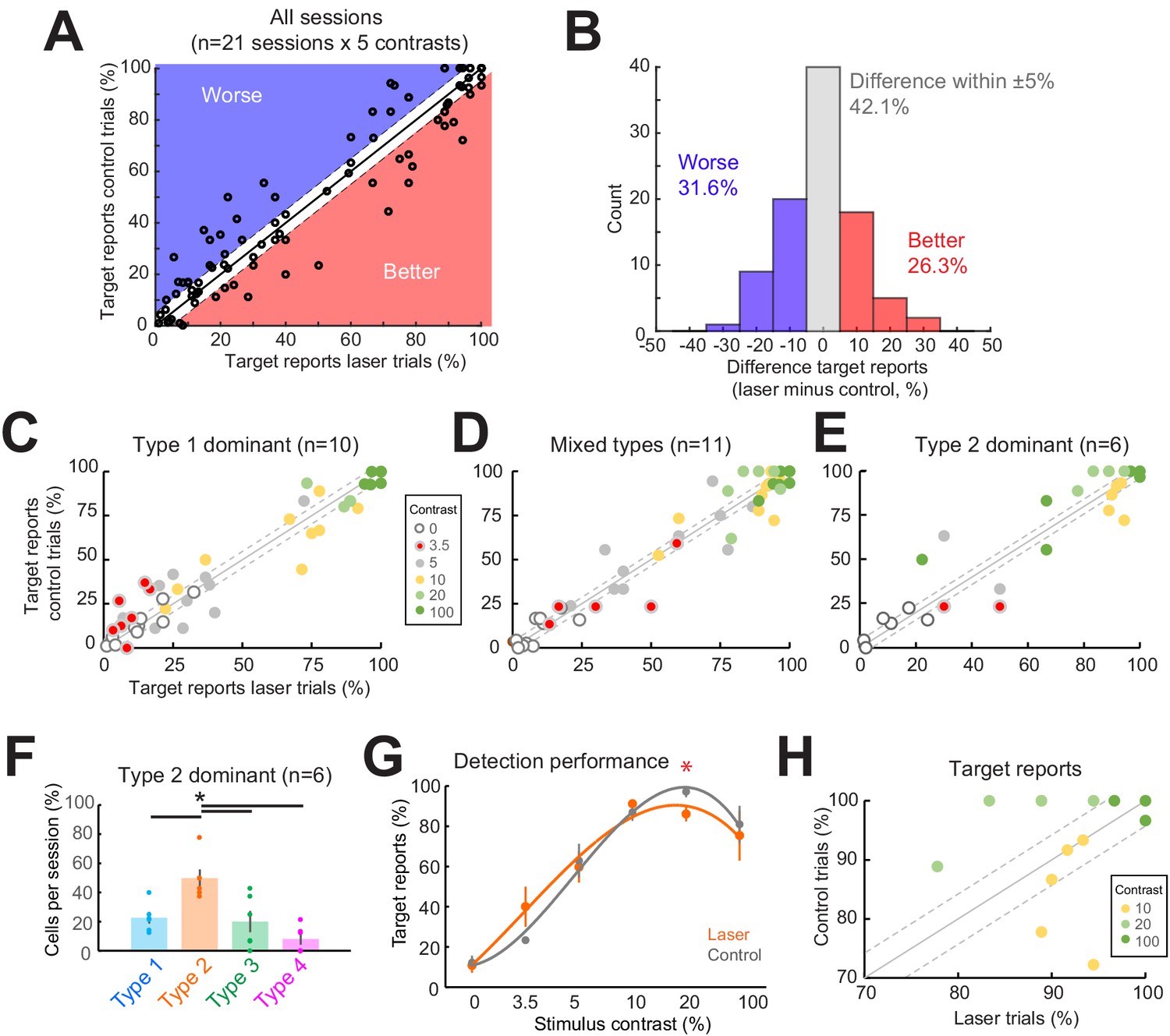
Behavioral task performance was heterogeneously affected on optogenetic suppression trials.
(A) Percent target reports across sessions and contrast conditions on laser (x-axis) and control (y-axis) trials. The diagonal unity line (solid black line) is flanked by ± 5%. Points above the diagonal (shaded blue) show instances where the laser impaired detection performance by >5%, while those below the diagonal show sessions where detection was improved on laser trials by >5%. (B) Histogram showing distribution of changes in behavioral responses across conditions (laser minus control trials) for the raw data shown in panel (A). (C–E) Target reports on laser (x-axis) and control (y-axis) trials across all contrasts for Type 1 dominant sessions (C), mixed-type sessions (D), and Type 2 dominant sessions (E). The unity line (solid gray diagonal) shows ± sem behavior responses across all contrasts in the control condition (flanking dashed diagonal lines). (F) Proportions of cell response types found with sessions containing greater than 35% Type 2 responses. Dots show individual sessions. Bar graphs show mean ± sem. *p = 0.0032, one-way Kruskal-Wallis (df = 3, Chi-sq = 13.8, post-hoc t-test). (G) Task performance on Type 2 dominant sessions showing percent of trials on which animals reported the presence of a visual stimulus on laser (orange) and control (gray) trials. *p = 0.016, t-test, paired, two-way. Session counts per contrast, ascending (left to right), are 6, 2, 6, 6, 4, and 6. Points show mean ± sem. Fits are third-order polynomials. (H) Target reports for individual Type 2 dominant sessions for 10% (yellow), 20% (light green), and 100% (dark green). The unity line (solid gray diagonal) shows ± sem behavior responses across all contrasts and sessions in the control condition (flanking dashed diagonal lines).
Figure 5—figure supplement 2
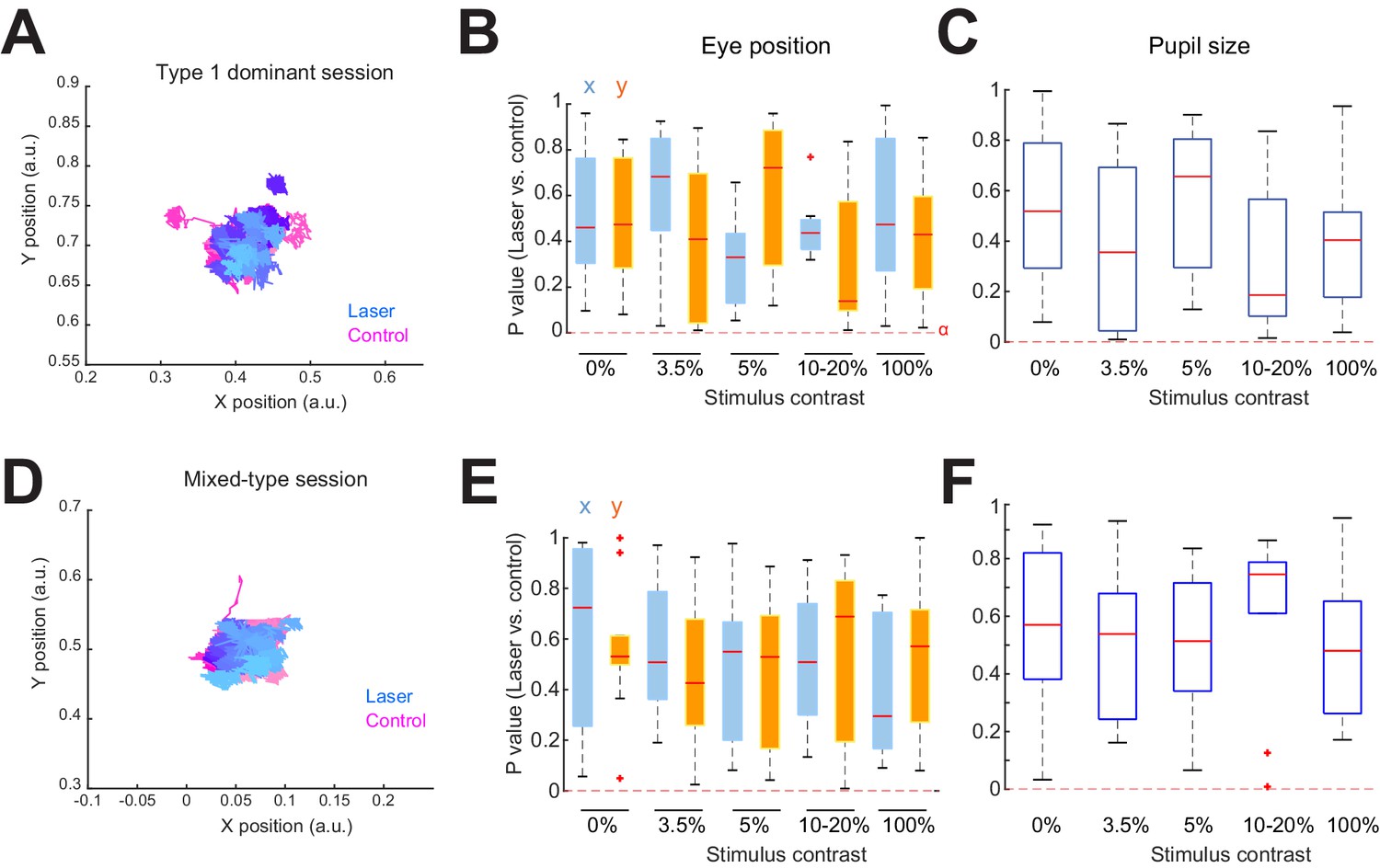
Eye position and pupil size do not account for differences in behavioral performance between Type 1 and mixed-type sessions.
(A–C) Type 1 dominant sessions. (A) Eye position traces from an example Type 1 dominant session during a 300 ms stimulus period for all 3.5% contrast trials on laser (blues) and control (pinks). Color shades denote individual trials. (B) Distribution of p-values (Wilcoxon rank sum test) comparing eye coordinate positions between laser and control trials across sessions. Box edges show 25th and 75th percentiles, whiskers extend to extreme data points, and the red center line shows the median. Dashed horizontal red line shows the Bonferroni-corrected alpha value for comparisons across all contrasts (α = 0.000417). Eye position was not significantly different between laser and control trials at any stimulus contrast condition for any session. (C) Same conventions as in panel (B), but comparing the average pupil size during the 300 ms laser/stimulus period. No statistically significant differences in pupil size with laser stimulation were observed under any condition. (D–F) Mixed-type sessions. (D) Eye position traces from an example mixed-type session for the 3.5% contrast trials. Same convention as in panel (A). (E) p-value distributions for mixed-type sessions (α = 0.000333). Same conventions as in panel (B). Eye position was not significantly different between laser and control trials at any stimulus contrast condition for any session. (F) Same as in panel (C), but for mixed-type sessions. Pupil size was not significantly different between control and laser trials under any condition.
Author response image 1
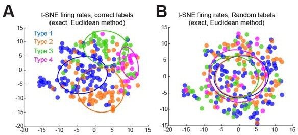
t-SNE results clustering firing rate differences (laser minus control) across all contrasts for all cells, labeled with ascribed labels (A), or with randomly ordered labels (B).
Error ellipses represent the covariance matrix and are centered on the median of tSNE results for each type.
Additional files
-
Transparent reporting form
- https://cdn.elifesciences.org/articles/66400/elife-66400-transrepform1-v2.pdf
-
Source data 1
- https://cdn.elifesciences.org/articles/66400/elife-66400-supp1-v2.zip
Download links
A two-part list of links to download the article, or parts of the article, in various formats.
Downloads (link to download the article as PDF)
Open citations (links to open the citations from this article in various online reference manager services)
Cite this article (links to download the citations from this article in formats compatible with various reference manager tools)
Heterogeneous side effects of cortical inactivation in behaving animals
eLife 10:e66400.
https://doi.org/10.7554/eLife.66400


