Interpreting wide-band neural activity using convolutional neural networks
- Kavli Institute for Systems Neuroscience, Centre for Neural Computation, The Egil and Pauline Braathen and Fred Kavli Centre for Cortical Microcircuits, NTNU, Norwegian University of Science and Technology, Norway
- Max-Planck-Insitute for Human Cognitive and Brain Sciences, Germany
- Cell & Developmental Biology, UCL, United Kingdom
- Institute of Behavioural Neuroscience, UCL, United Kingdom
- Open Climate Fix, United Kingdom
- DeepMind, United Kingdom
- Institute of Psychology, Leipzig University, Germany
Figures
Figure 1 with 11 supplements
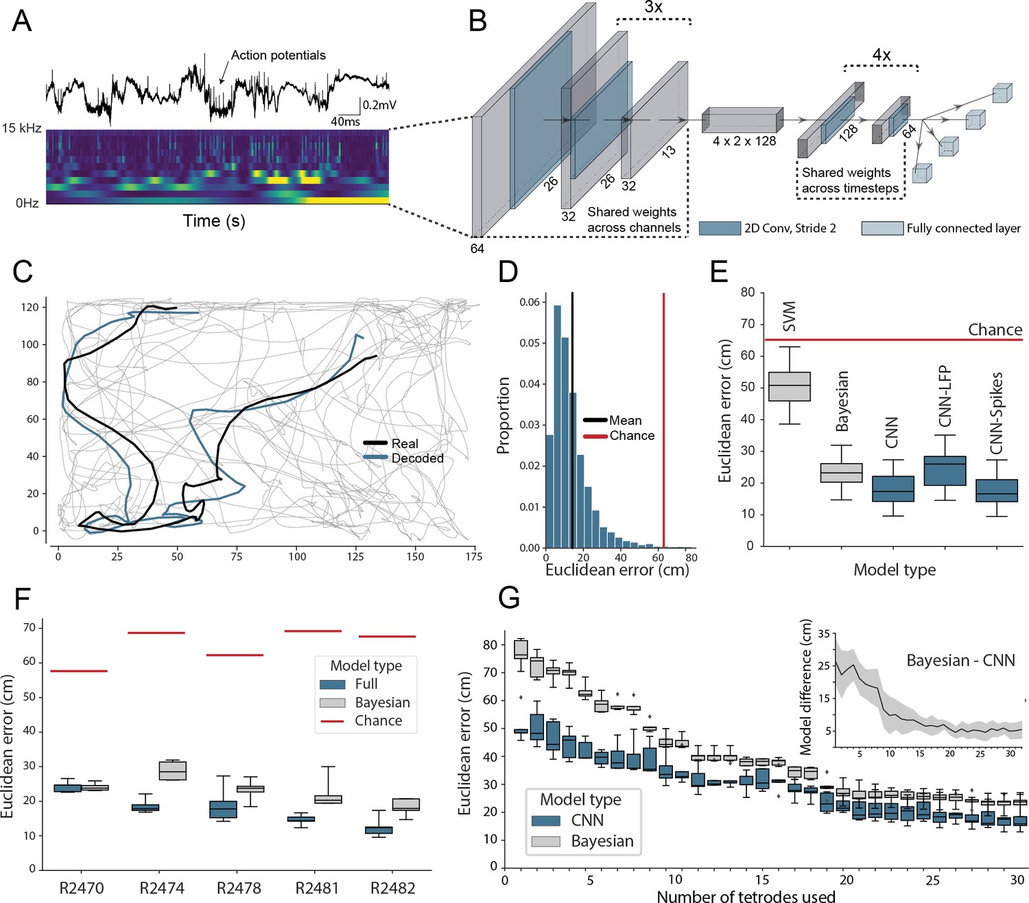
Accurate decoding of self-location from unprocessed hippocampal recordings.
(A) Top, a typical ’raw’ extracellular recording from a single CA1 electrode. Bottom, wavelet decomposition of the same data, power shown for frequency bands from 2 Hz to 15 kHz (bottom to top row). (B) At each timestep wavelet coefficients (64 time points, 26 frequency bands, 128 channels) were fed to a deep network consisting of 2D convolutional layers with shared weights, followed by a fully connected layer with a regression head to decode self-location; schematic of architecture shown. (C) Example trajectory from R2478, true position (black) and decoded position (blue) shown for 3 s of data. Full test-set shown in Figure 1—video 1. (D) Distribution of decoding errors from trial shown in (C), mean error (14.2 cm ± 12.9 cm, black), chance decoding of self-location from shuffled data (62.2 cm ± 9.09 cm, red). (E) Across all five rats, the network (CNN) was more accurate than a machine learning baseline (SVM) and a Bayesian decoder (Bayesian) trained on action potentials. This was also true when the network was limited to high-frequency components (>250Hz, CNN-Spikes). When only local frequencies were used (<250Hz, CNN-LFP), network performance dropped to the level of the Bayesian decoder (distributions show the fivefold cross validated performance across each of five animals, n=25). Note that this likely reflects excitatory spikes being picked up at frequencies between 150 and 250 Hz (Figure 1—figure supplement 2). (F) Decoding accuracy for individual animals, the network outperformed the Bayesian decoder in all cases. An overview of the performance of all tested models can be seen in Figure 1—figure supplement 3. (G) The advantage of the network over the Bayesian decoder increased when the available data was reduced by downsampling the number of channels (data from R2478). Inset shows the difference between the two methods.
Figure 1—figure supplement 1
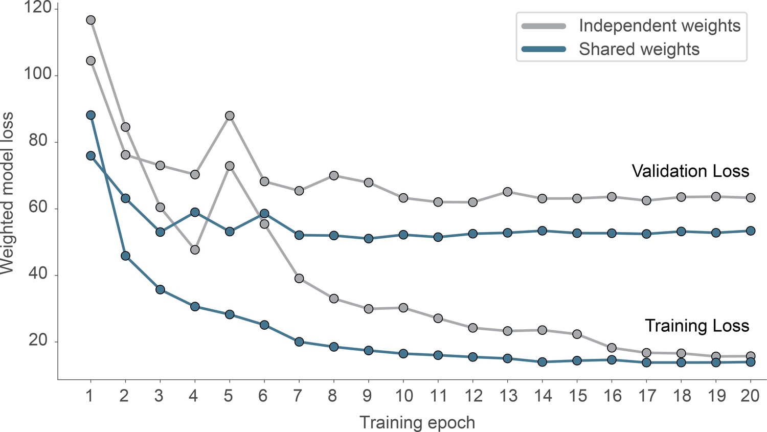
Effect of weight sharing on model performance.
We evaluated two models on the same dataset, using either shared weights and 2D-convolutions (blue) or independent weights using 3D-convolutions (gray).The model using shared weights reaches a lower validation loss and generalizes better (smaller overfit).
Figure 1—figure supplement 2
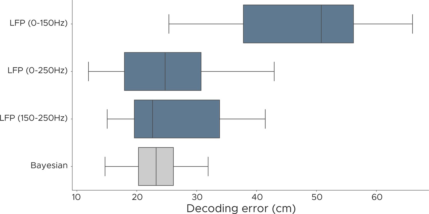
Decoding performance of LFP models.
We evaluated the decoding performance of the LFP model using different frequency components and show euclidean error scores for positional decoding. Each model was fully cross-validated across all five animals, using a different set of frequencies. LFP (0–150 Hz) uses 12/26 frequencies, LFP (0–250 Hz) uses 15/26 frequencies, LFP (150–250 Hz) uses 3/26 frequencies, Bayesian decoder uses spike sorted data.
Figure 1—figure supplement 3
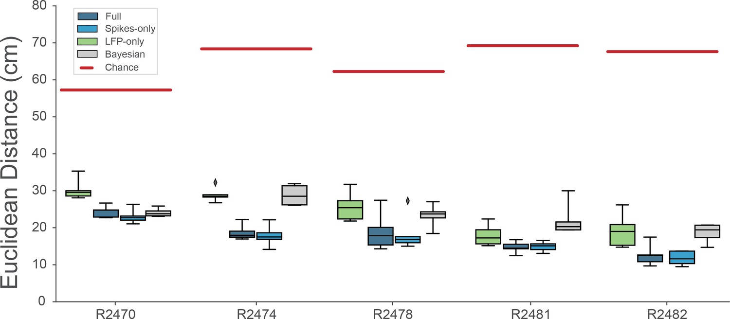
Decoding performance across different models.
We calculated the Euclidean distance between the real behavior and decoded behavior across five rats and four different models. Full model has access to all frequency bands from 2 to 15,000 Hz, Spikes model has access to frequencies >250Hz, while LFP model uses frequencies <250Hz. Bayesian decoder was trained on spike sorted data. Chance level is indicated as red line.
Figure 1—figure supplement 4
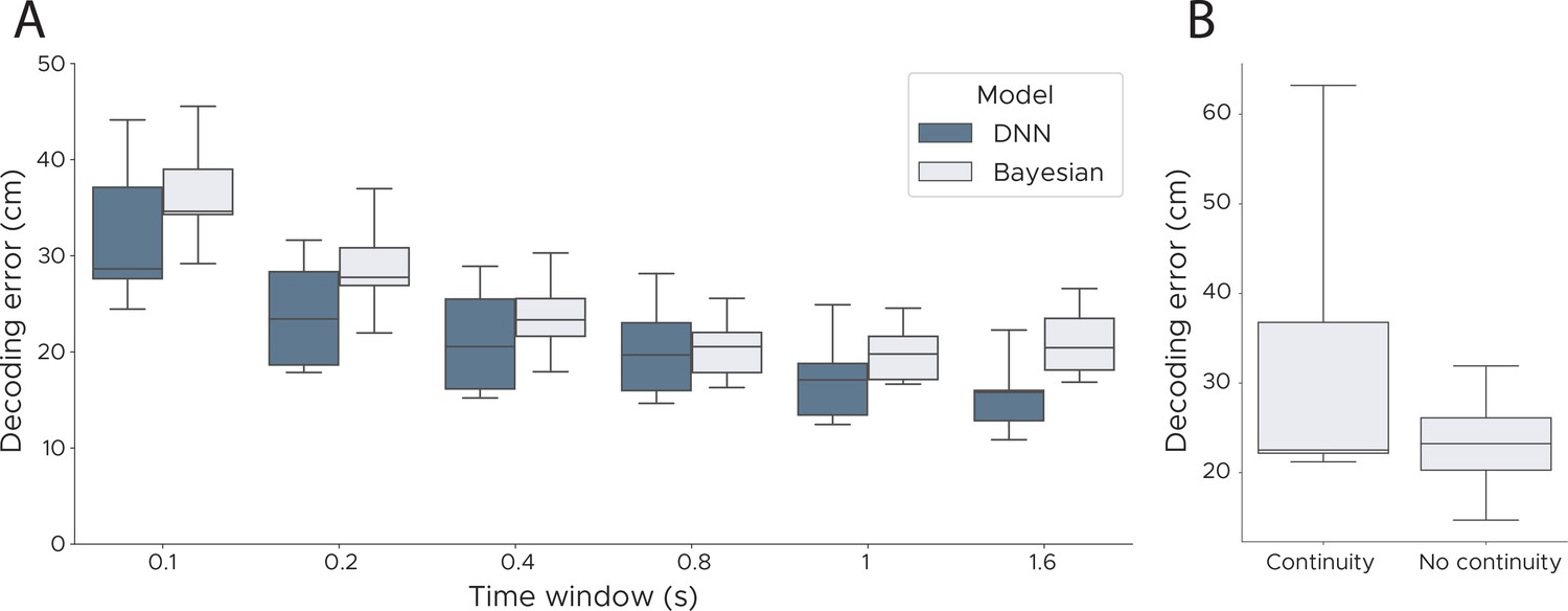
Decoding performance across time windows and continuity priors.
(A) We evaluated the performance of our model and a Bayesian decoder using a range of different durations (0.1 s - 1.6 s). Our model outperformed the Bayesian decoder for all lengths of the time window, with both models tending to be more accurate with larger windows. (B) We assessed Bayesian decoding with and without a continuity prior. The prior was implemented as a Gaussian distribution centred around the previous decoded location adjusting the standard deviation based on the speed in the previous timestep. Compared to the model with no continuity prior the model with such a prior has a higher variance across animals and makes more ‘catastrophic’ errors though has a marginally lower median error (median decoding error with continuity, 22.51 cm; without continuity, 23.23 cm). We show box plots across five cross-validations and all five animals.
Figure 1—figure supplement 5
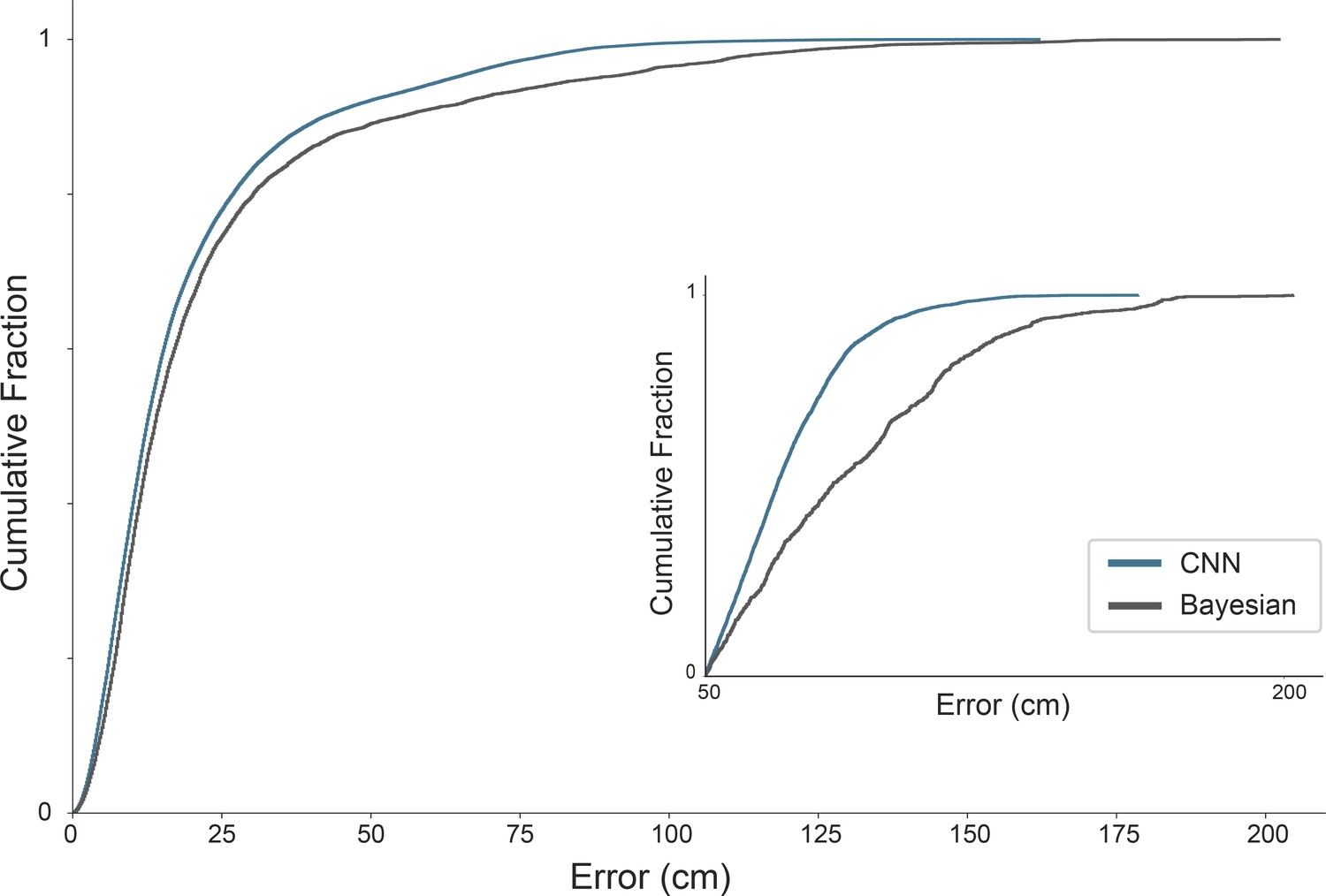
Difference in error distribution between Bayesian decoder and CNN.
Cumulative error distribution of decoding errors for Bayesian decoder (blue) and CNN (gray) for euclidean errors between true position and decoded position. Inset shows error distribution for decoding errors higher than 50 cm. Data from one animal (R2478).
Figure 1—figure supplement 6
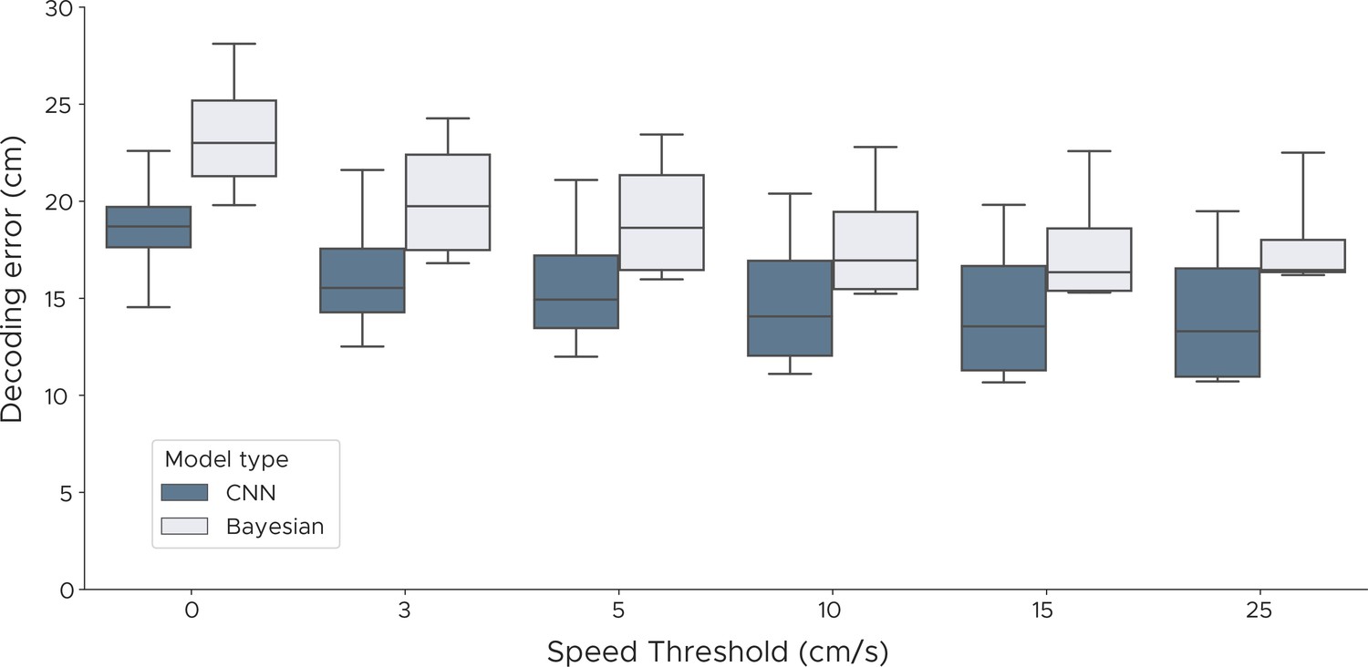
Decoding performance with different speed thresholds.
We evaluated both the Bayesian decoder and the convolutional neural network errors across different speed thresholds to investigate if periods of immobility adversely affect decoding performance. For each speed threshold, we discarded samples where the speed of the animal was below the threshold, using speeds from 0 cm/s up to 25 cm/s. We show box plots across five cross-validations and all five animals.
Figure 1—figure supplement 7
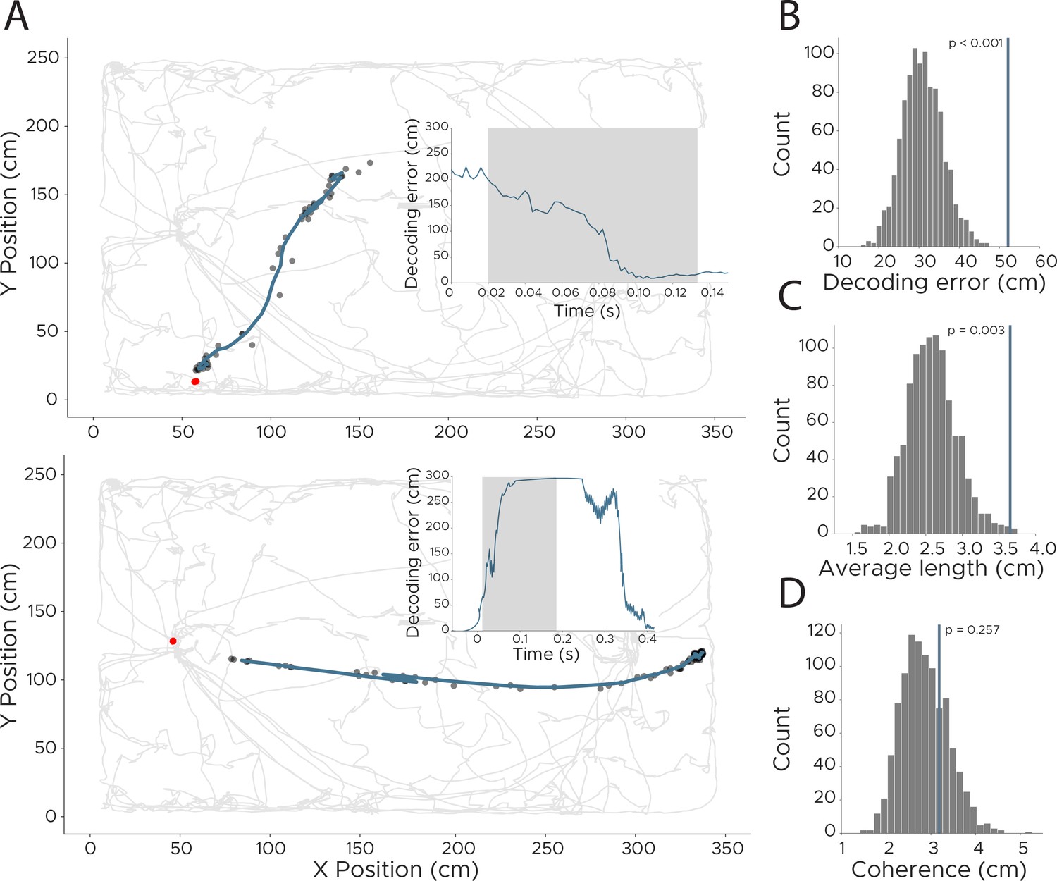
Detection of replay events in CA1 recordings.
To detect more fine-grained representations, we retrained the model using a lower downsampling rate, resulting in an effective sampling rate of 500 Hz. This allowed us to investigate model behavior at timepoints of manually extracted replay events. (A) Two example replay events with model loss indicated in inset. Shaded area across model loss indicates timepoints of replay event. Model loss of 0 indicates accurate decoding of animals position. Real position of the animal is indicated as a red dot (note that the animal was not moving during these times so the real position did not change), while decoded position (smoothed using a 0.02 s kernel) is shown in dark blue, with unsmoothed positions shown as black dots. (B–D) We quantified replay events using three different measures to separate them from non-replay events. To obtain a statistical score for all three, we shuffled the replay events in time (keeping the absolute length of each replay) and recalculated each measure 1000 times. Original value is indicated as a dark blue line. (B) We evaluated if replay events show a higher overall decoding error by calculating the average loss during the replay event (n=1000, p<0.001). (C) We calculated the average length of each replay event to detect if replay events are longer than the average trajectory (n=1000, p=0.003). (D) We also calculated if replay events are as coherent as other parts of the decoding by calculating the difference to a polynomial fitted to the trajectory (n=1000, p=0.257).
Figure 1—figure supplement 8
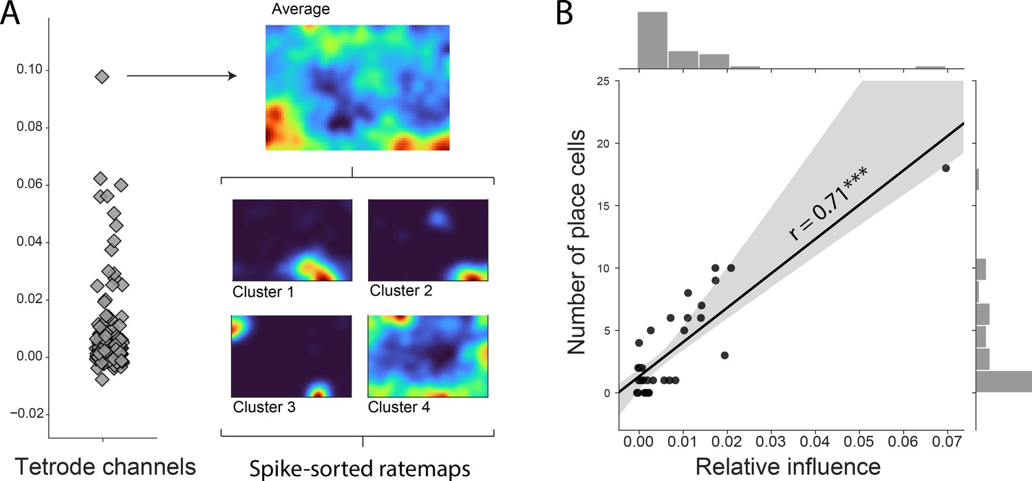
Influence of decoding across channels.
(A) Channel influence scores for positional decoding (left). The most influential channel for the positional decoding has a high number of place cells (right). Average ratemap of all clusters (top, n=21) and four example clusters (bottom) shown. (B) Influence scores per tetrode (average influence over four channels) highly correlates with number of place cells on the tetrode, indicating that the network is correctly identifying place cells as the spatially most informative neural correlate.
Figure 1—figure supplement 9

A subset of frequency pairs exhibit greater than expected decoding influence.
We evaluated 325 frequency pairs to investigate the relative influence of conjoint frequencies versus the sum of their individual influence on the decoding of position. (A) For each frequency pair, the combined influence – calculated by shuffling both together () – is compared to the summed influence of each alone (). Lower triangle shows , upper triangle shows . Positive, red, entries in lower triangular indicate frequency pairs with a combined influence greater than the sum of their individual influences. (B) Same a left matrix with non-significant entries removed. (C) p Values for the data in the left matrix determined using the Wilcoxon signed rank test, Holm-Sidak corrections were applied for n=325 comparisons. There was a limited subset of frequency pairings in which the combinatorial influence on position decoding significantly exceeded the sum of individual frequencies – these were focused on the bands associated with place cell action potential (331.5–937.5 Hz) and to a lesser extent on the ones associated with putative interneurons.
Figure 1—figure supplement 10
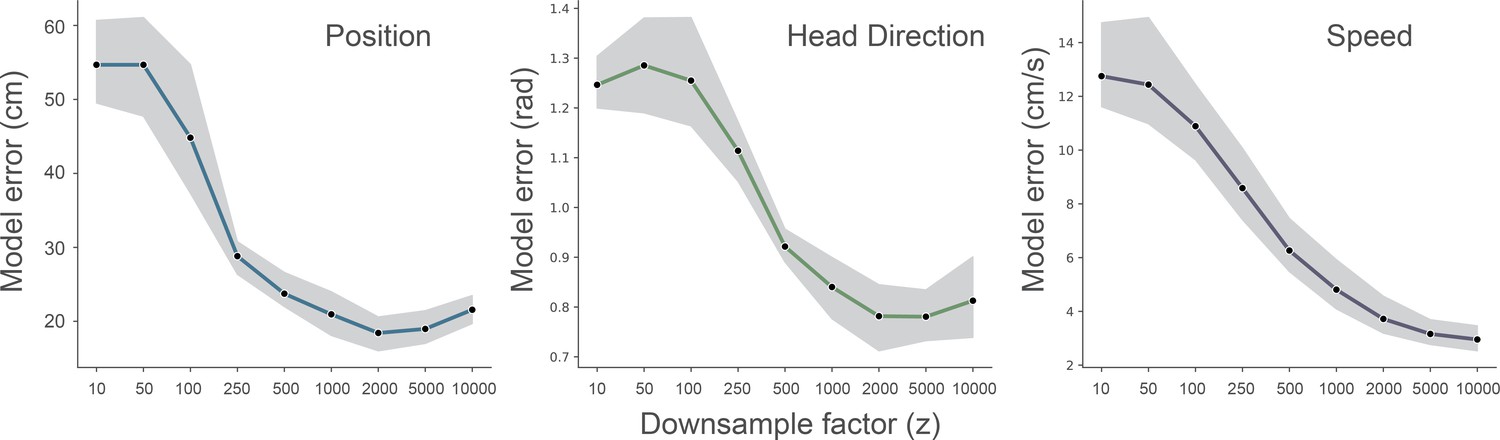
Effect of downsampling on model performance.
We ran fully cross-validated experiments for different downsampling values of the wavelet transformed electrophysiological signal (z = [10…10000]). Data from one animal (R2478), the shaded area indicates the 95% confidence interval.
Figure 1—video 1
Decoding of multiple behaviors from rodent CA1.
We show the decoding errors on the fully cross-validated test set of one example animal, from a model which was simultaneously decoding position, head direction and speed. Left part shows the decoding of position on top of the animal trajectory, top right shows the decoding of head direction and bottom right shows the decoding of speed on top of a histogram of decoded speeds.Real behavior is indicated in green, decoded output behavior is shown in red.
Figure 2 with 1 supplement
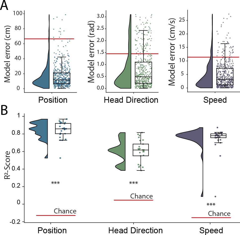
Simultaneous decoding of multiple variables from hippocampal data.
(A) Position, head direction, and running speed were accurately decoded in concert by a single network. Data from all five animals, each point indicates an error for a single sample. The red dashed line indicates the chance level obtained by shuffling the input relative to the output while fully retraining the model. (B) -scores, a loss-invariant measure of model performance – ranging from 1 (perfect decoding) to negative infinity – allowing performance to be compared between dissimilar variables. Data as in (A), each point corresponds to one of five cross-validations within each of five rats.
Figure 2—figure supplement 1

Running speed linearly correlates with power in multiple frequency bands.
To identify simple relationships between behavioral variables and frequency bands, we calculated the Spearman Rank Order Correlation Coefficient (speed and position) and Circular Correlation (head direction) between the wavelet transformed electrophysiological signal and the position, head direction and speed of the animal. (A) In the case of running speed, multiple frequency bands exhibited moderate correlations. In particular, as previously reported, the strongest relationship was present in the theta-band (10.36 Hz, rho = 0.415), a relationship that was present in all five rats (p < 0.01). (B,C) In contrast no such relationship was found for the other spatial variables. Indeed, the strongest correlation identified was a negative relationship between x-axis position and power in the theta-band (10.36 Hz, rho=-0.0759, but which was not significant, p = 0.9803). Gray points indicate correlation for each animal (n=5), bold line shows the mean of those.
Figure 3 with 3 supplements
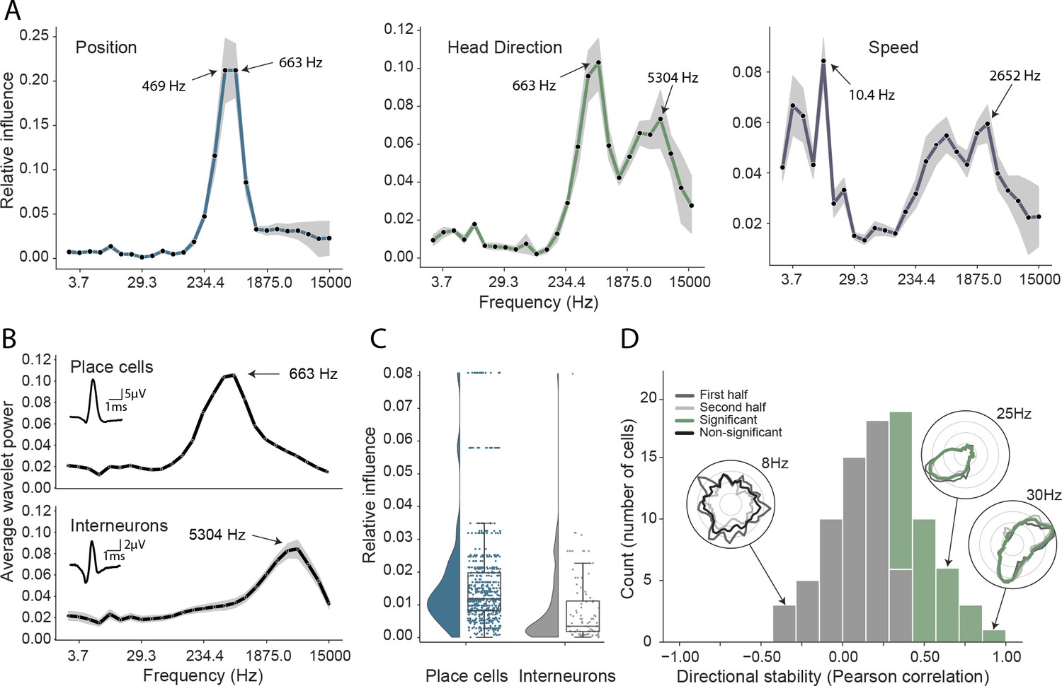
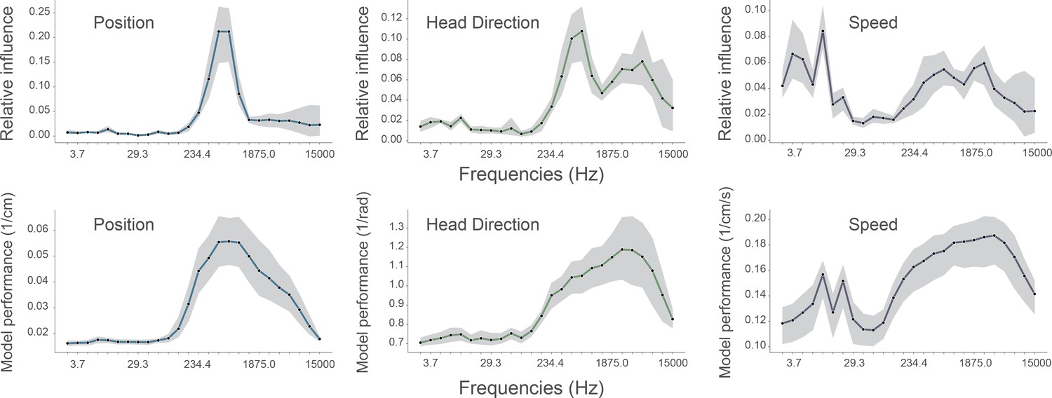
Analysis of trained network identifies informative elements of the neural code.
(A) A shuffling procedure was used to determine the relative influence of different frequency bands in the network input. Left, the 469 Hz and 663 Hz components – corresponding to place cell action potentials – were highly informative about animals’ positions. Middle, both place cells and putative interneurons (5304 Hz) carried information about head direction. Right, several frequency bands were informative about running speed, including those associated with the LFP (10.4 Hz) and action potentials. Data from all animals. (B) Wavelet coefficients of place cell (top) and interneuron (bottom) waveforms are distinct and correspond to frequencies identified in A. Inset, average waveforms. Data from all animals. (C) Frequency bands associated with place cells (469 and 663 Hz) were more informative about position than those associated with putative interneurons (5304 Hz) – their elimination produced a larger decrement in decoding performance (p<0.001). Data from all animals. (D) A subset of putative CA1 interneurons encodes head direction. Thirty-three of 91 interneurons from five animals exhibited pronounced directional modulation that was stable throughout the recording (green). Depth of modulation quantified using Kullback-Leibler divergence vs. uniform circle. Stability assessed with the Pearson correlation between polar ratemaps from the first and second half of each trial (dark gray and light gray). Cells with p<0.01 for both measures were considered to be reliably modulated by head direction. Inset, example polar ratemaps. Data from all animals.
Figure 3—figure supplement 1
Performance of standard model compared with models trained on single frequency bands.
To determine if the frequencies identified as important by our complete model matched those that were most informative on their own, we compared the influence plots (top row, same as Figure 3A in manuscript) generated for the standard model with accuracy plots from models trained on individual frequency bands (bottom row). In all cases, 128 channel recordings from rodent CA1 were used to decode position (left column), head direction (middle column), and speed (right column). Influence plots were constructed as before. Accuracy (bottom row) is simply defined as 1/decoding error and is not normalized relative to chance or ceiling performance, values were generated using the same convolutional neural network while only providing a single frequency band for training and testing. Although influence is not expected to be a simple linear function of accuracy, the results from the two methods were highly correlated: position, Spearman’s ρ=0.88 (p<0.001); head direction, ρ=0.82 (p<0.001); running speed, ρ=0.47 (p=0.02). For each frequency band, we show the average cross-validation performance across five animals for three different behaviors and loss functions. Data from all animals, the shaded area indicates the 95% confidence interval.
Figure 3—figure supplement 2
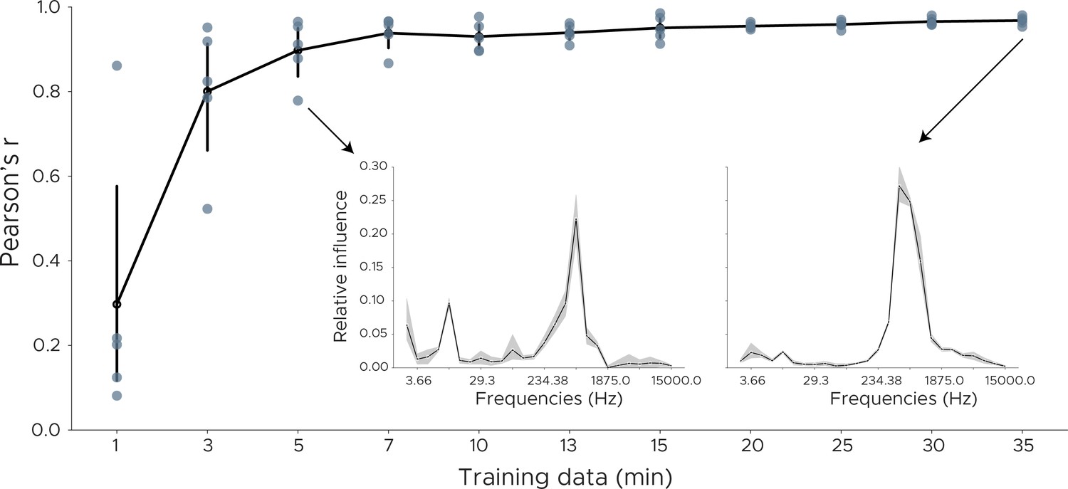
Decoding influence for downsampled models.
To measure the robustness of the influence measure we downsampled the training data and retrained the model using cross-validation. We plot the Pearson correlation between the original influence distribution using the full training set and the influence distribution obtained from the downsampled data. Each dot shows one cross-validation split. Inset shows influence plots for two runs, one for 35 min of training data, the other in which model training consisted of only 5 min of training data.
Figure 3—figure supplement 3

Decoding influence for simulated behaviors.
(A) We quantified our influence measure using simulated behaviors. We used the wavelet preprocessed data from one CA1 recording and simulated two behavioral variables which were modulated by two frequencies (58 Hz and 3750 Hz) using different multipliers (B). We then trained the model using cross-validation and calculated the influence scores via feature shuffling.
Figure 4 with 1 supplement
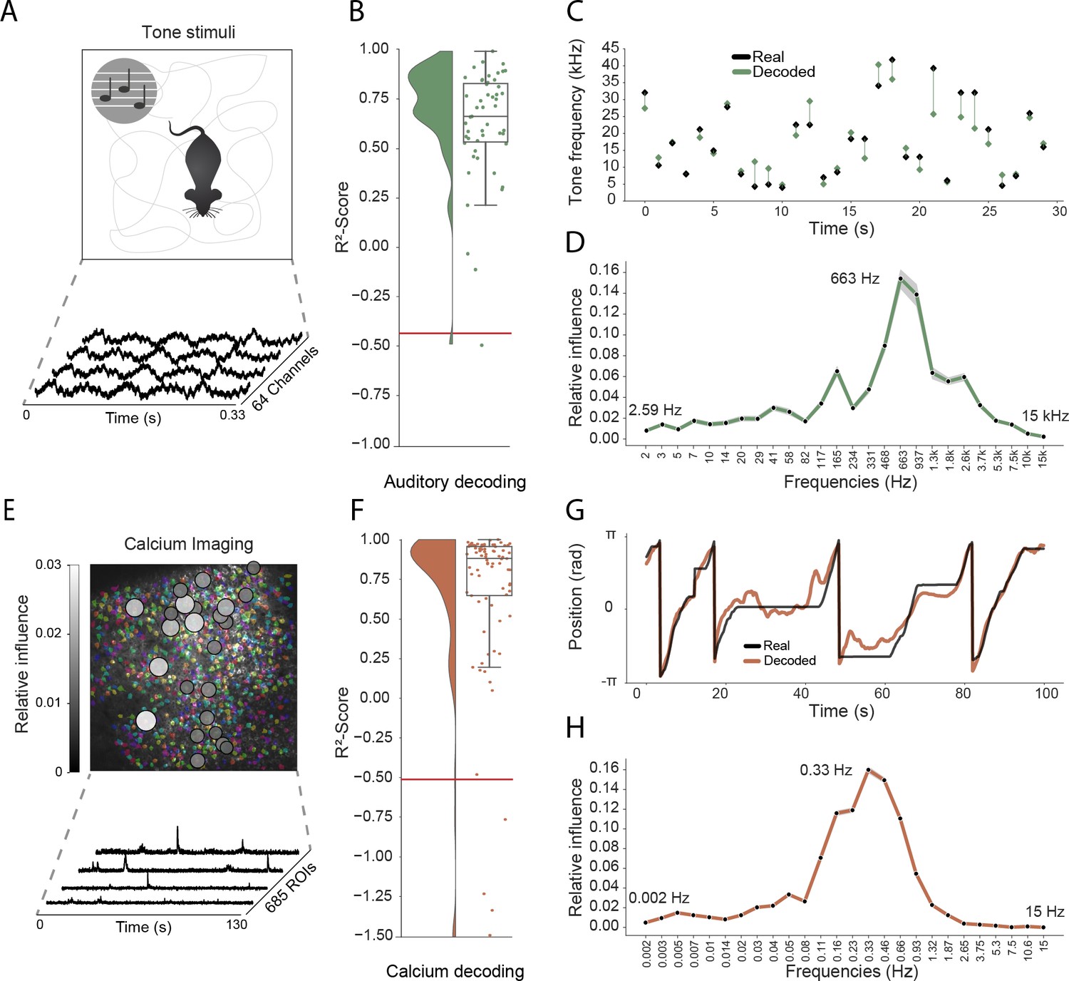
Model generalizes across recording techniques and brain regions.
(A) Overview of auditory recording. We recorded electrophysiological signals while the mouse is freely moving inside a small enclosure and is presented with pure tone stimuli ranging from 4 kHz to 64 kHz. (B) -score for decoding of frequency tone from auditory cortex (0.73 ± 0.08). Each dot describes the -score for a 5 s sample of the experiment. Chance level is indicated by the red line. (C) An example section for decoding of auditory tone frequencies from auditory electrophysiological recordings, real tone colored in black, decoded tone in green, the line between real and decoded indicates magnitude of error. (D) Influence plots for decoding of auditory tone stimuli, same method as used for CA1 recordings. (E) Calcium recordings from a mouse running on a linear track in VR. We record from 685 cells and use Suite2p to preprocess the raw images and extract calcium traces which we feed through the model to decode linear position. Overlay shows relative influence for decoding of position calculated for each putative cell. (F) -score for decoding of linear position from two-photon CA1 recordings (0.90 ± 0.03). Each dot describes the -score for a 5 s sample of the experiment. Chance level is indicated by the red line. (G) Example trajectory through the virtual linear track (linearized to with real position (black) and decoded position (orange)). (H) Influence plots for decoding of position from two-photon calcium imaging. Note that the range of frequencies is between 0 Hz and 15 Hz as the sampling rate of the calcium traces is 30 Hz.
Figure 4—figure supplement 1
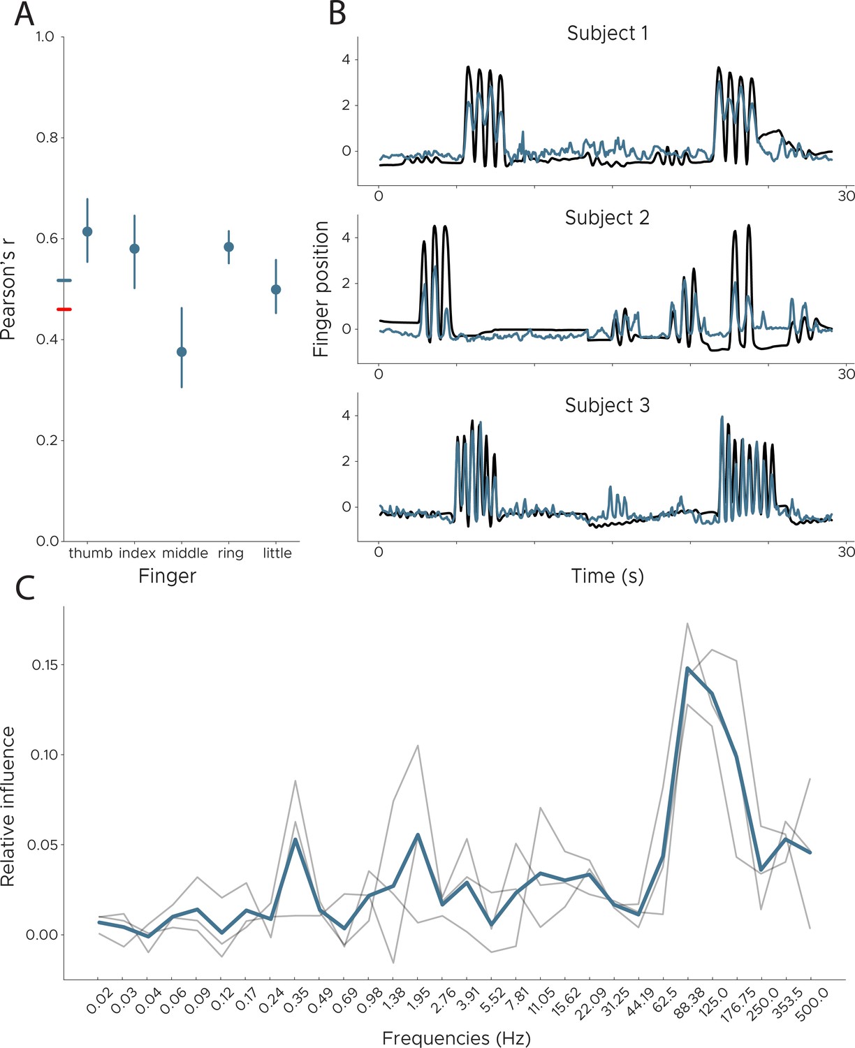
Decoding finger movements from human ECoG recordings.
We applied DeepInsight to a publicly available ECoG dataset in order to decode finger movement from three subjects. (Left) We show Pearson’s r across subjects split into individual fingers. The colored line on the y-axis shows the average performance for our model (blue) and the best competing model (black). (Right) Example decoding results across all subjects. The blue line is the decoded finger position, while the black line shows ground truth information obtained via a data glove. Data from BCI Competition IV, Dataset 4 (Schalk et al., 2007), comparison model from Cortex Team, Research Centre INRIA (see competition results). (C) Influence plots for the decoding of finger movement from ECoG data, calculated by shuffling each frequency and recalculating the error. Each line depicts one participant, with the average shown in blue. Peak influence is located at 88 Hz, followed by 125 Hz.
Additional files
-
Supplementary file 1
Layer by layer architecture of the convolutional model.
Note that the first layers 1–8 share the weights over the channel dimension while layers 9–15 share the weights across the time dimension. Layers 9 to 15 depict the kernel sizes and strides for the tetrode recordings with 128 channels. For recordings with different number of channels we adjust the number of downsampling layers to match the dimension of layer 15. Order of dimensions: Time, Frequency, Channels.
- https://cdn.elifesciences.org/articles/66551/elife-66551-supp1-v1.xlsx
-
Transparent reporting form
- https://cdn.elifesciences.org/articles/66551/elife-66551-transrepform-v1.pdf
Download links
A two-part list of links to download the article, or parts of the article, in various formats.
Downloads (link to download the article as PDF)
Open citations (links to open the citations from this article in various online reference manager services)
Cite this article (links to download the citations from this article in formats compatible with various reference manager tools)
Interpreting wide-band neural activity using convolutional neural networks
eLife 10:e66551.
https://doi.org/10.7554/eLife.66551


