Computational modeling of cambium activity provides a regulatory framework for simulating radial plant growth
- Centre for Organismal Studies, Heidelberg University, Germany
- Department of Agricultural Sciences, Università degli Studi di Napoli Federico II, Italy
- Gregor Mendel Institute, Vienna Biocenter, Austria
- Mathematical Institute, Leiden University, Netherlands
- Institute of Biology, Leiden University, Netherlands
- BioQuant, Heidelberg University, Germany
Figures
Figure 1
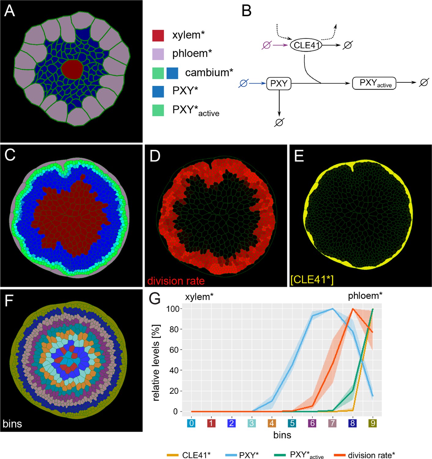
Generation of the initial model.
(A) Tissue template used to run VirtualLeaf simulations. Phloem* is depicted in purple, xylem* in red. Cambium cells* are colored according to their levels of PXY* and PXY-active*. Cambium* is colored in blue due to the initial level of PXY*. Color legend on the right applies to (A) and (C). (B) Schematic representation of the biochemical model. Reactions that occur in all cell types* are drawn in black. Reactions only occurring in the phloem* are depicted in purple, reactions specific to the cambium* are in blue. Crossed circles represent production or degradation of molecules. (C) Output of simulation using Model 1. (D) Visualization of cell division rates* within the output shown in (C).Dividing cells* are marked by red color fading over time. (E) Visualization of CLE41* levels within the output shown in (C).(F) Sorting cells* within the output shown in (C)into bins based on how far their centers are from the center of the hypocotyl*. Different colors represent different bins. (G) Visualization of the relative chemical levels and division rates in different bins shown in (F)averaged over n = 10 simulations of Model 1. Each chemical’s bin concentration is first expressed as a percentage of the maximum bin value of the chemical and then averaged over all simulations. The colored area indicates the range between minimum and maximum value of the relative chemical concentration. Bin colors along the x-axis correspond to the colors of bins in (F).The shading represents the range between minimal and maximal values during simulations.
Figure 2 with 1 supplement
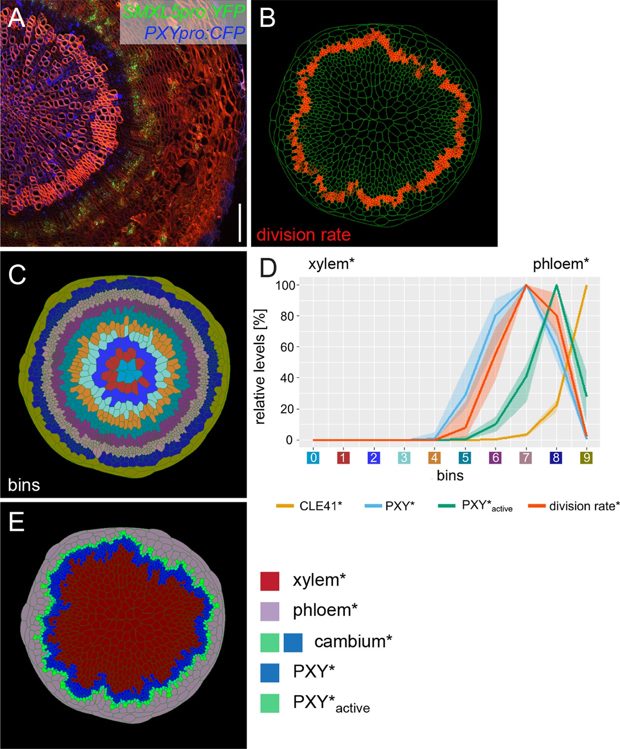
Implementing phloem formation into the model.
(A) Cross-section of a wild-type hypocotyl expressing PXYpro:CFP (blue) and SMXL5pro:YFP (green). Cell walls are stained by Direct Red 23, mainly visualizing xylem (red). Only a sector of the hypocotyl is shown with the center on the left. Scale bar: 100µm. Ten samples were analysed in total with similar results. An image version for color-blind readers is provided in Figure 2—figure supplement 1. (B) Visualization of cell division rates* within the output shown in (C, E).Dividing cells* are marked by red color fading over time. (C) Sorting cells* within the output shown in (B, E)into bins. (D) Visualization of the average relative chemical levels* and division rates* in different bins of repeated simulations of Model 2A (n = 10). Bin label colors along the x-axis correspond to the colors of bins shown in (C).The shading represents the range between minimal and maximal values during simulations. (E) Output of simulation using Model 2A. Unlike Model 1 (Figure 1C), Model 2A produces new phloem cells*.
Figure 2—figure supplement 1
Wild type control for fluorescent reporter analyses and color-blind modes for images shown in main figures.
(A) A hypocotyl cross-section from a wild-type plant not carrying any transgene, which was stained and imaged in the same way as, for example, the section shown in Figure 2A. The signal detected in the outermost cell layer applying the microscope settings used for detecting PXYpro:CFP activity (in blue) originates from autofluorescence possibly due to suberin deposition in that cell layer. Scale bar: 100 μm. (B–D) Images shown in Figure 2A and Figure 3A–E, respectively, in which the red color was replaced by magenta. Size bars: see respective main figures.
-
Figure 2—figure supplement 1—source data 1
Raw image data collected for Figure 2—figure supplement 1.
- https://cdn.elifesciences.org/articles/66627/elife-66627-fig2-figsupp1-data1-v2.zip
Figure 3 with 6 supplements
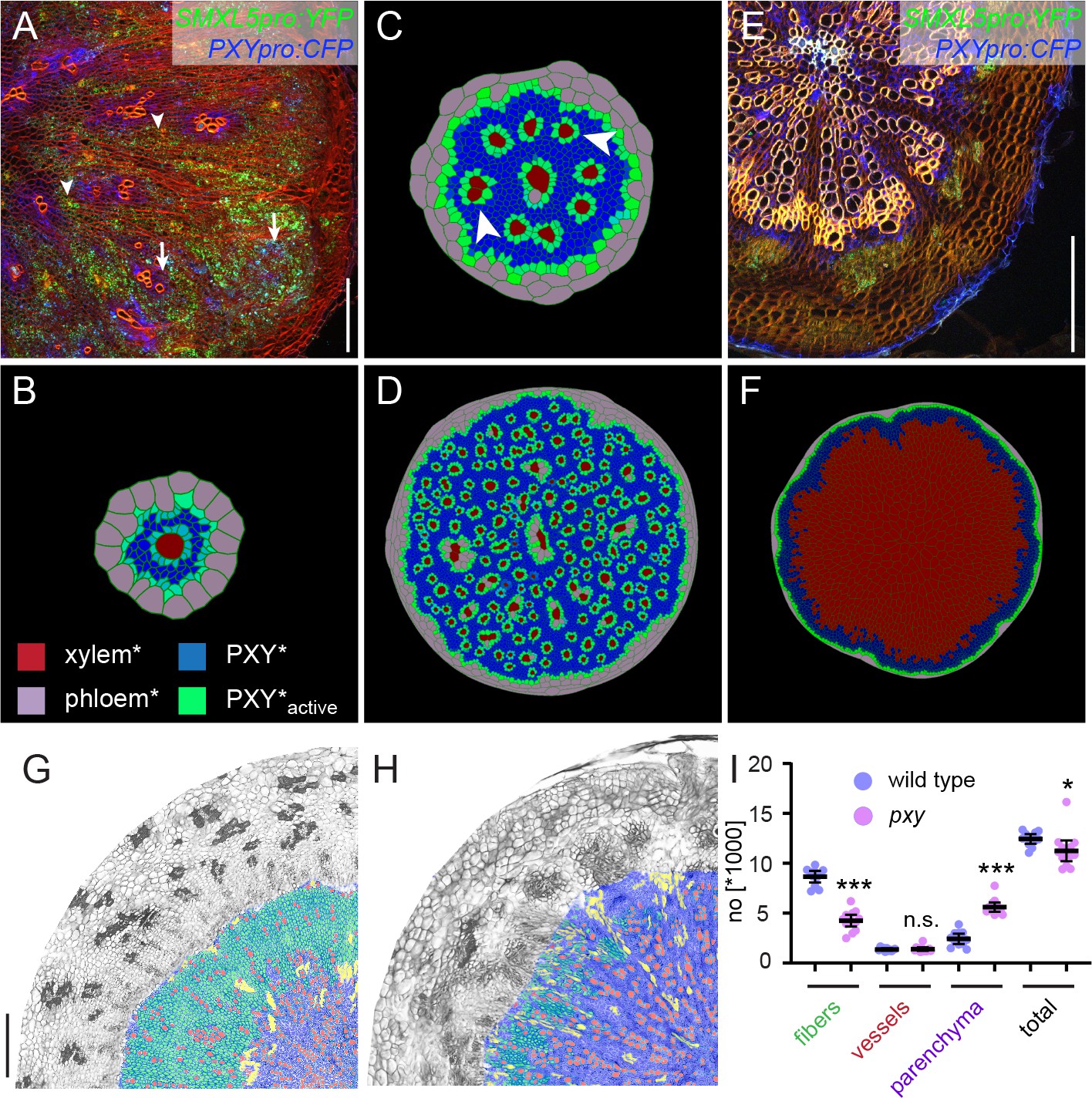
Comparing the effect of perturbing cambium activity in the model and in plants.
(A) Cross-section of a hypocotyl carrying PXYpro:CFP (blue), SMXL5pro:YFP (green) markers, and the IRX3pro:CLE41 transgene. Cell walls are stained by Direct Red 23 visualizing mostly xylem (red). Arrowheads point to proximal hypocotyl regions where SMXL5pro:YFP activity is found. Arrows indicate distal regions with SMXL5pro:YFP activity. Cell walls are stained by Direct Red 23 visualizing mostly xylem (red). Only a quarter of the hypocotyl is shown with the center in the upper-left corner. Scale bar: 100µm. Ten samples were analysed in total with similar results. An image version for color-blind readers is provided in Figure 2—figure supplement 1. (B) First frames of Model 2B simulations. Due to the expression of CLE41* by xylem cells*, high levels of PXY-active* are generated around xylem cells* already at this early stage. Legend in (B) indicates color code in (B, C, D, F). (C) Intermediate frames of Model 2B simulations. Newly formed xylem cells* express CLE41* and produce high levels of PXY-active* next to them (white arrowheads). (D) The final result of Model 2B simulations. Zones of PXY* (blue) and PXY-active* (green) are intermixed, xylem cells* are scattered, and phloem cells* are present in proximal areas of the hypocotyl*. (E) Cross-section of a pxy mutant hypocotyl carrying PXYpro:CFP (blue) and SMXL5pro:YFP (green) markers, stained by Direct Red 23 (red). The xylem shows a ray-like structure. Only a quarter of the hypocotyl is shown with the center in the upper-left corner. Ten samples were analysed in total with similar results. Scale bar: 100µm. An image version for color-blind readers is provided in Figure 2—figure supplement 1. (F) Final result of Model 2D simulations. Reducing PXY* levels leads to similar results as produced by Model 1 (Figure 1C) where only xylem* is produced. (G, H) Comparison of histological cross-sections of a wild-type (G)and a pxy (H)mutant hypocotyl, including cell-type classification produced by ilastik. The ilastik classifier module was trained to identify xylem vessels (red), fibers (green), and parenchyma (purple), unclassified objects are shown in yellow. Size bar in G: 100 µm. Same magnification in G and H. (I) Comparison of the number of xylem vessels, fibers, and parenchyma cells found in wild-type (blue) and pxy mutants (purple). Welch’s t-test was performed comparing wild-type and pxy mutants for the different cell types (n = 11–12). ***p<0.0001, *p<0.05. Lines indicate means with a 95% confidence interval. 11 (wild type) and 13 (pxy) samples were analysed.
-
Figure 3—source data 1
Source data for cell type classification using ilastik.
- https://cdn.elifesciences.org/articles/66627/elife-66627-fig3-data1-v2.zip
Figure 3—figure supplement 1
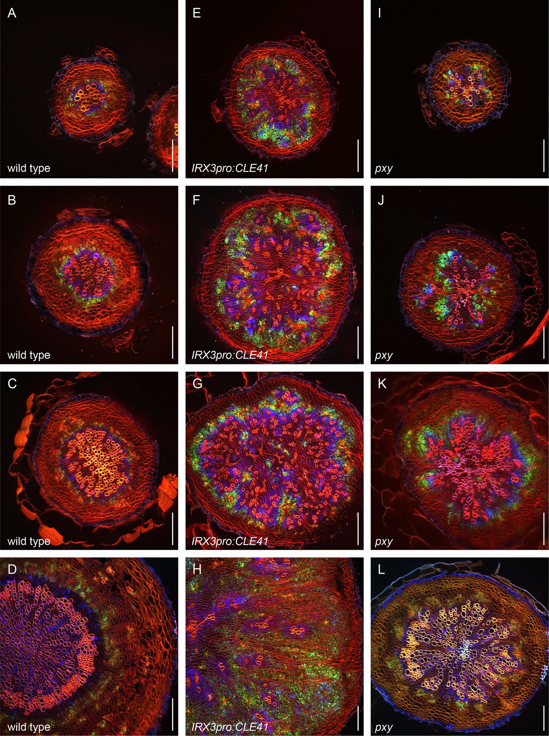
First example revealing the dynamics of PXYpro:CFP/SMXL5pro:YFP activities during radial hypocotyl growth in wild-type, IRX3pro:CLE41, and pxy plants.
(A–D) PXYpro:CFP (blue) and SMXL5pro:YFP (green) activities at different stages of wild-type hypocotyl development from young (A)to old (D).(E–H) PXYpro:CFP (blue) and SMXL5pro:YFP (green) activities at different stages of hypocotyl development in IRX3pro:CLE41 plants from young (A)to old (D).(I–L) PXYpro:CFP (blue) and SMXL5pro:YFP (green) activities at different stages of hypocotyl development in pxy mutants from young (A)to old (D).Sections are stained by Direct Red 23 (red). Scale bars: 100µm. Note that pictures (D, H, L) are also depicted in Figure 2 and Figure 3. A version of this figure for color-blind readers is provided in Figure 3—figure supplement 3. Five (A-CT, E-G, I-K) or ten (D, H, L) samples were analysed in total with similar results.
-
Figure 3—figure supplement 1—source data 1
Raw image data collected for Figure 3—figure supplement 1, first part.
- https://cdn.elifesciences.org/articles/66627/elife-66627-fig3-figsupp1-data1-v2.zip
-
Figure 3—figure supplement 1—source data 2
Raw image data collected for Figure 3—figure supplement 1, second part.
- https://cdn.elifesciences.org/articles/66627/elife-66627-fig3-figsupp1-data2-v2.zip
Figure 3—figure supplement 2
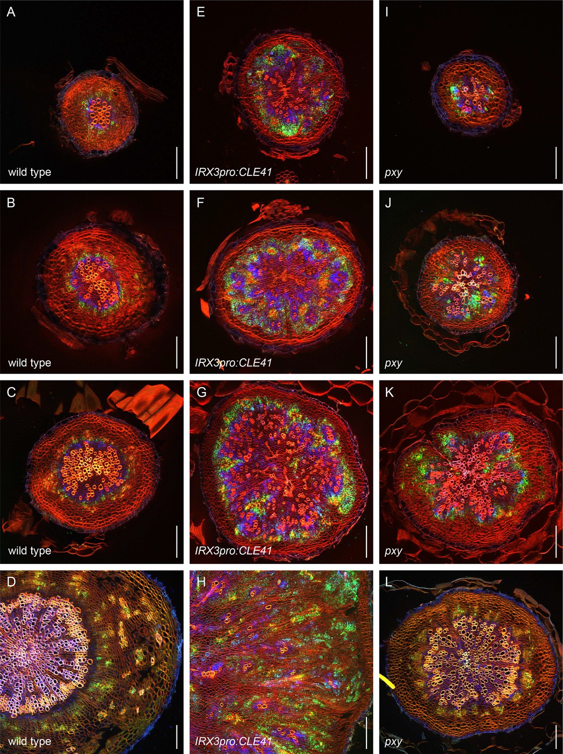
Second example revealing the dynamics of PXYpro:CFP/SMXL5pro:YFP activities during radial hypocotyl growth in wild-type, IRX3pro:CLE41, and pxy plants.
(A–D) PXYpro:CFP (blue) and SMXL5pro:YFP (green) activities at different stages of wild-type hypocotyl development from young (A)to old (D).(E–H) PXYpro:CFP (blue) and SMXL5pro:YFP (green) activities at different stages of hypocotyl development in IRX3pro:CLE41 plants from young (A)to old (D).(I–L) PXYpro:CFP (blue) and SMXL5pro:YFP (green) activities at different stages of hypocotyl development in pxy mutants from young (A)to old (D).Sections were stained by Direct Red 23 (red). Scale bars: 100µm. A version of this figure for color-blind readers is provided in Figure 3—figure supplement 4. Ten (A-C, E-G, I-K) or five (D, H, L) samples were analysed with similar results.
-
Figure 3—figure supplement 2—source data 1
Raw image data collected for Figure 3—figure supplement 2, first part.
- https://cdn.elifesciences.org/articles/66627/elife-66627-fig3-figsupp2-data1-v2.zip
-
Figure 3—figure supplement 2—source data 2
Raw image data collected for Figure 3—figure supplement 2, second part.
- https://cdn.elifesciences.org/articles/66627/elife-66627-fig3-figsupp2-data2-v2.zip
Figure 3—figure supplement 3
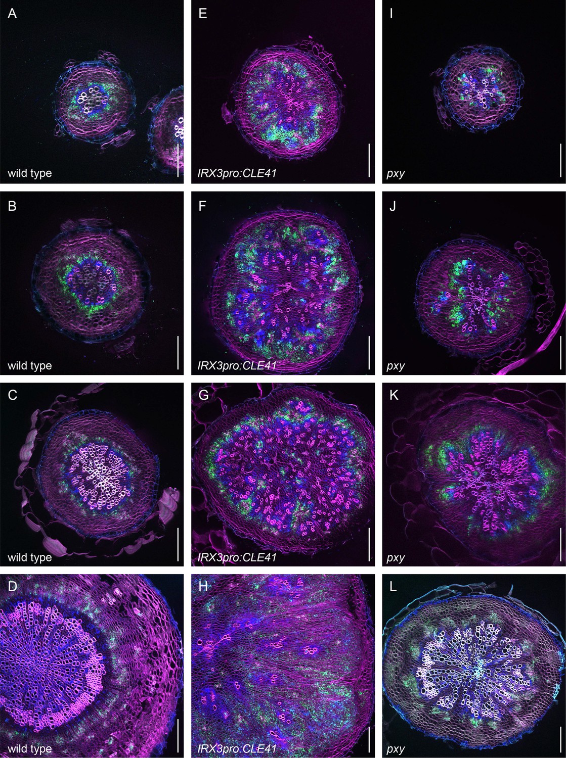
First example revealing the dynamics of PXYpro:CFP/SMXL5pro:YFP activities during radial hypocotyl growth in wild-type, IRX3pro:CLE41, and pxy plants (color-blind mode).
(A–D) PXYpro:CFP (blue) and SMXL5pro:YFP (green) activities at different stages of wild-type hypocotyl development from young (A)to old (D).(E–H) PXYpro:CFP (blue) and SMXL5pro:YFP (green) activities at different stages of hypocotyl development in IRX3pro:CLE41 plants from young (A)to old (D).(I–L) PXYpro:CFP (blue) and SMXL5pro:YFP (green) activities at different stages of hypocotyl development in pxy mutants from young (A)to old (D).Sections are stained by Direct Red 23 (red). Scale bars: 100µm. Note that pictures (D, H, L) are also depicted in Figure 2 and Figure 3. Five (A-C, E-G, I-K) or ten (D, H, L) were analysed with similar results.
Figure 3—figure supplement 4
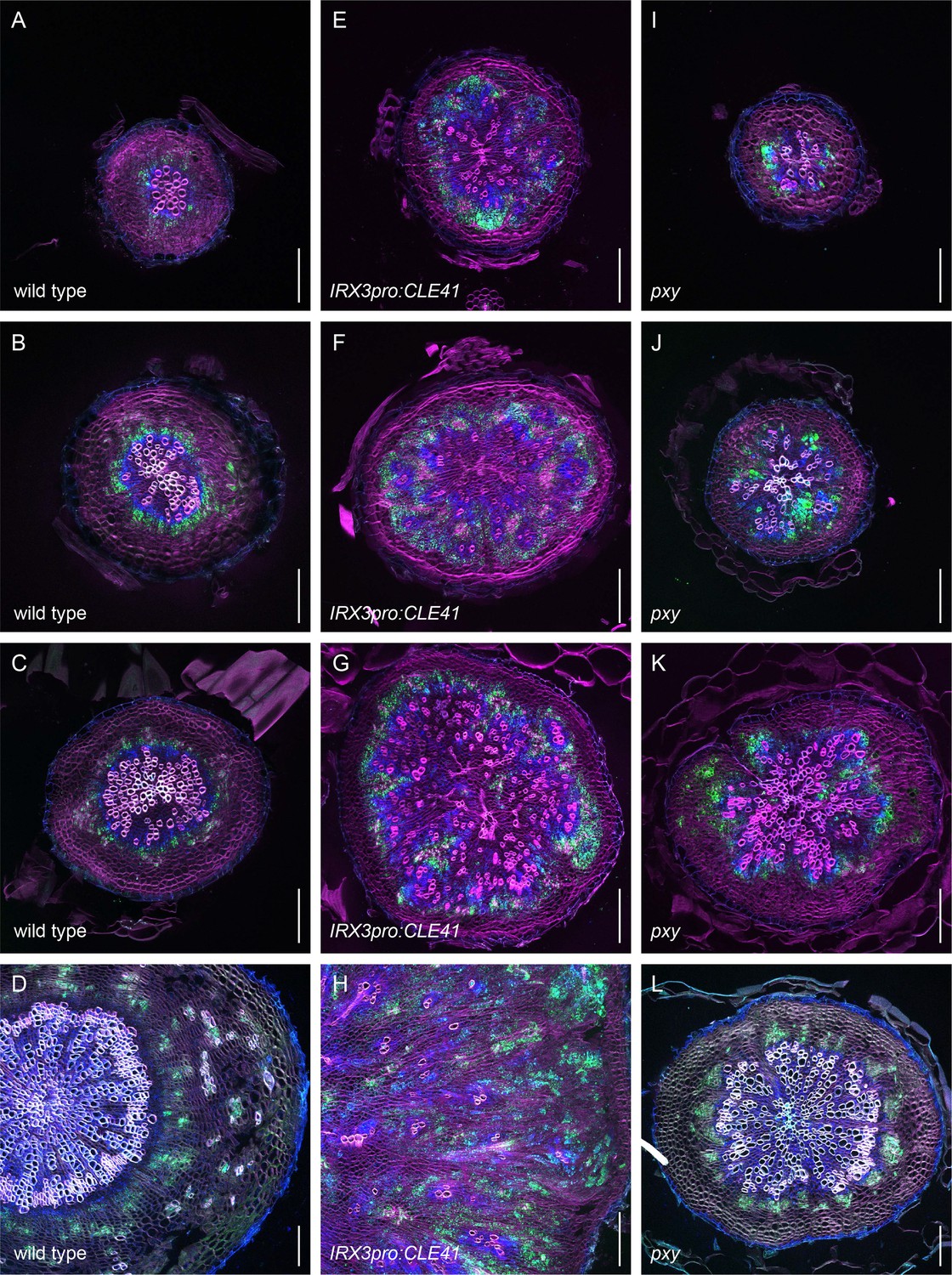
Second example revealing the dynamics of PXYpro:CFP/SMXL5pro:YFP activities during radial hypocotyl growth in wild-type, IRX3pro:CLE41, and pxy plants (color-blind mode).
(A–D) PXYpro:CFP (blue) and SMXL5pro:YFP (green) activities at different stages of wild-type hypocotyl development from young (A)to old (D).(E–H) PXYpro:CFP (blue) and SMXL5pro:YFP (green) activities at different stages of hypocotyl development in IRX3pro:CLE41 plants from young (A)to old (D).(I–L) PXYpro:CFP (blue) and SMXL5pro:YFP (green) activities at different stages of hypocotyl development in pxy mutants from young (A)to old (D).Sections were stained by Direct Red 23 (red). Scale bars: 100µm. Five (A-C, E-G, I-K) or ten (D, H, L) samples were analysed with similar results.
Figure 3—figure supplement 5

Close-up revealing the dynamics of PXYpro:CFP/SMXL5pro:YFP activities in hypocotyls in wild-type and pxy plants.
(A–C) Three examples showing PXYpro:CFP (top, bottom, in magenta) and SMXL5pro:YFP (middle, bottom, in green) activities in the cambium zone of wild-type plants. Scale bar in (A): 20µm. Same magnification in (A–F). (D–F) Three examples showing PXYpro:CFP (top, bottom, in magenta) and SMXL5pro:YFP (middle, bottom, in green) activities in the cambium zone of pxy mutants. Note that Direct Red 23 staining (in gray) is only shown in top and middle imageds but not in ‘merged’ images at the bottom. Shown are late stages as depicted in Figure 3—figure supplement 1C and K and Figure 3—figure supplement 2C and K. Ten samples were analysed in total with similar results.
Figure 3—figure supplement 6
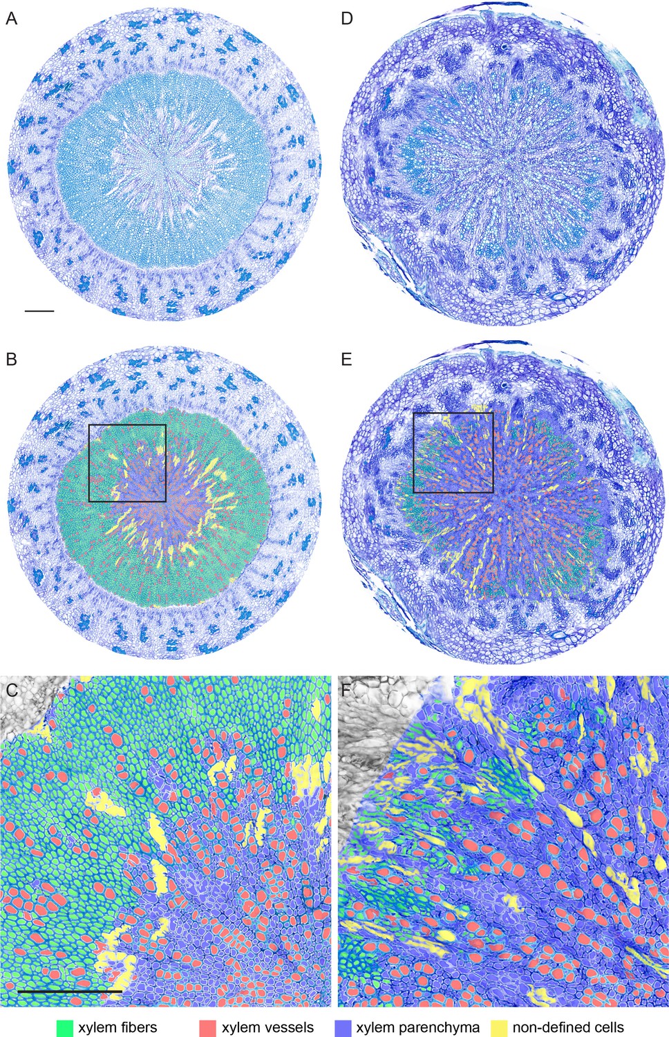
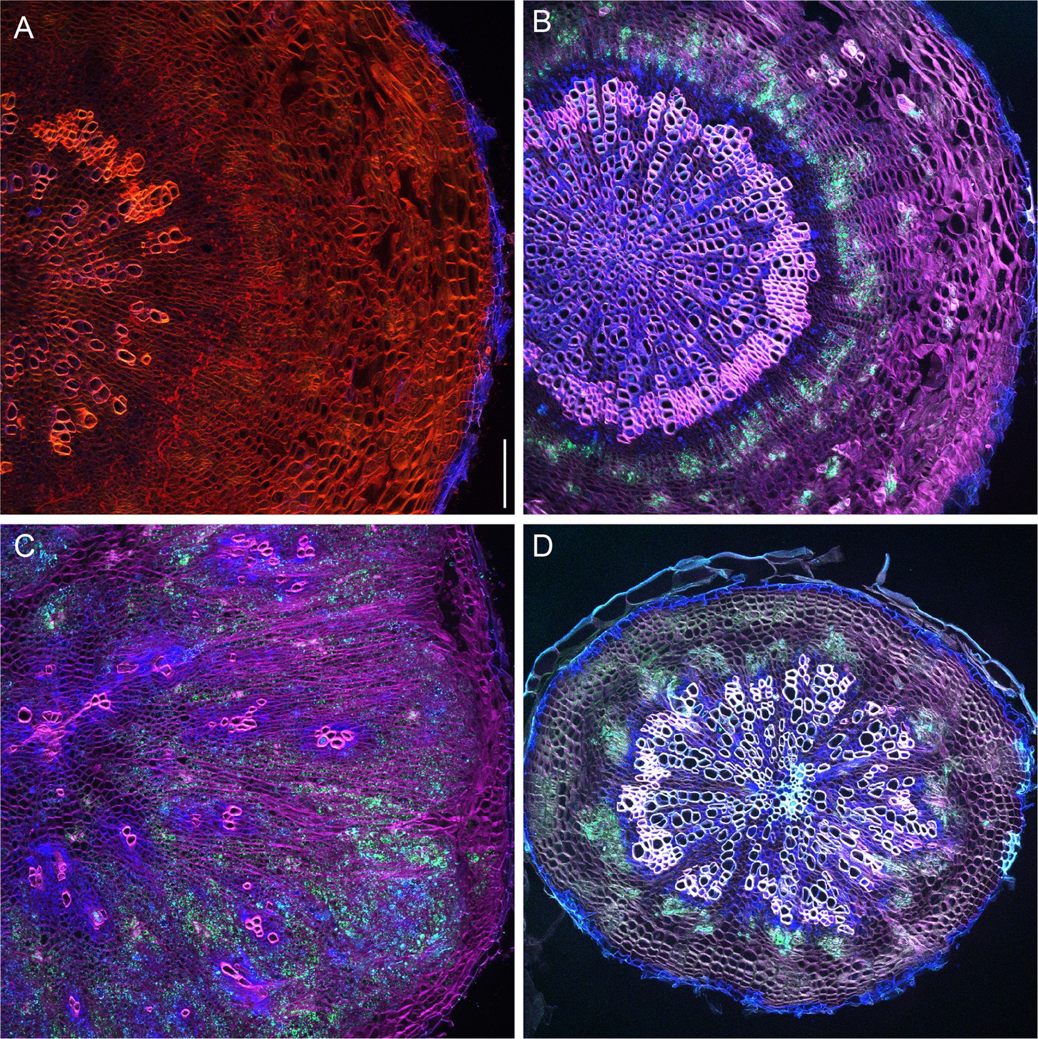
Overview and magnifications of sections used for cell-type classification shown in Figure 3.
Original toluidine-stained cross-sections (A, D), cross-section with cell-type classifications (B, E), and magnifications of regions indicated by black rectangles in (B) and (E) (C, F)for wild type (A–C)and pxy mutants (D–F)are shown. Cell-type classification was exclusively performed in the xylem area. Size bars in A and C: 100 µm. Same magnification in A, B, D, E and in C and F, respectively. 11 (wild type) and 13 (pxy) samples were anaysed.
Figure 4 with 3 supplements
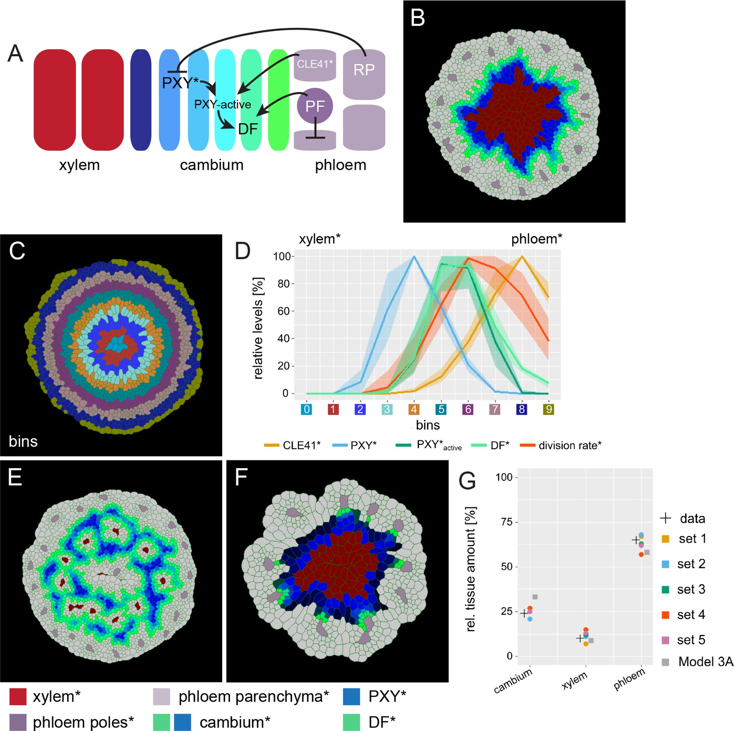
An extended model for simulating genetic perturbations of cambium activity.
(A) Regulatory network proposed based on experimental observations. (B) Result of the simulation run for Model 3A. This model implements the network interactions described in (A). Color coding at the bottom of Figure 4. (C) Outline of cell bins for the results of Model 3A, as shown in (B).(D) Visualization of the relative levels of chemicals* and division rates* in different bins. Bin colors along the x-axis correspond to the bin colors in (C).The shading represents the range between minimal and maximal values during simulations (n = 10). (E) Output of Model 3B simulation. Ectopic CLE41* expression was achieved by letting xylem cells* produce CLE41*. (F) Output of Model 3C. Simulation of the pxy mutant was achieved by removing the stimulation of DF* production by PXY* and hence by removing the effect of PXY* on cell division and cambium* subdomain patterning. Because of the network structure, PXY* can be eliminated from Model 3 without letting the model collapse (Figure 3F) but reproducing the pxy mutant phenotype observed in adult hypocotyls (Figure 4E). Be aware that cell* proliferation is generally impaired under these conditions reducing overall template growth*. Because the final output covers the same image area, cell size seems to be enlarged which, however, is not the case. (G) Estimated tissue ratios for five identified parameter sets compared to experimental values (‘data’) found for wild type hypocotyls 20d after germination (Sankar et al., 2014) and compared to the final model output before the automated parameter search (’Model 3A’) and the implementation of experimentally determined cell wall thickness for xylem* and phloem*.
Figure 4—figure supplement 1
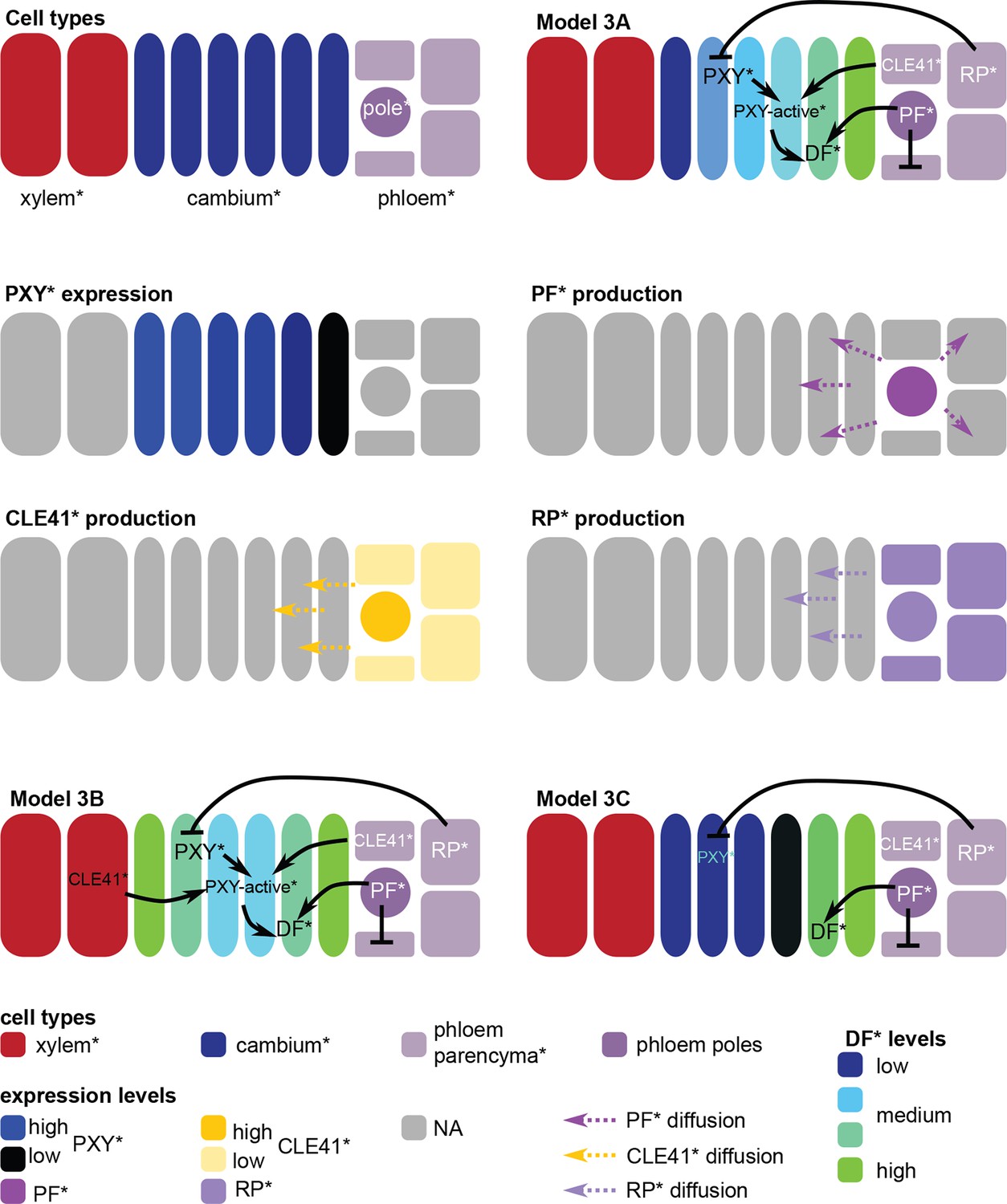
Overview of cell types*, regulatory interactions and expression* profiles in Model 3.
Schemes include representations for Models 3B and C. Color code shown at the bottom of the figure.
Figure 4—figure supplement 2
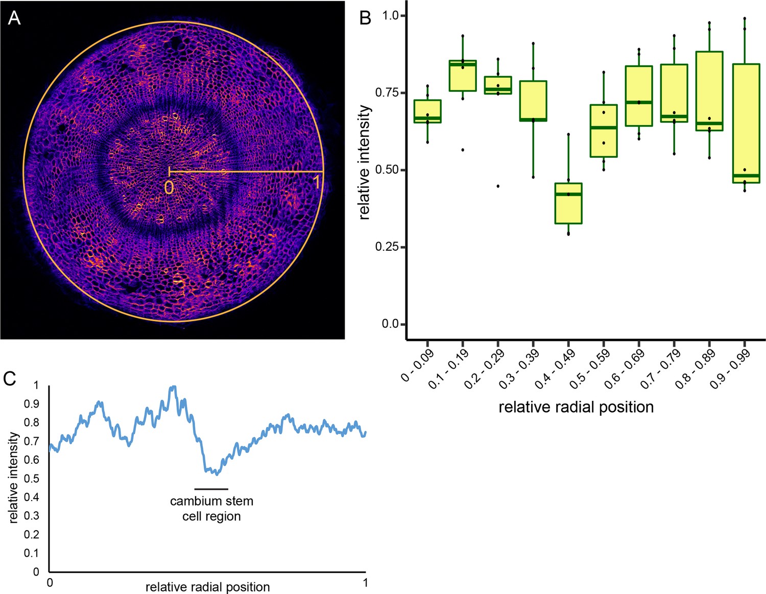
Determination of cell wall thickness across the radial sequence of hypocotyl tissues.
(A) Cross-section of a 4.5-week-old plant stained by Direct Red 23. Radius and circumference used by the ‘Radial Profile’ function of the Fiji image analysis tool (Schindelin et al., 2012) are indicated. Note that the function uses the whole circle area for analysis. (B) Plot of six Direct Red 23-stained cross-sections analyzed by the ‘Radial Profile’ function of Fiji. Staining intensity and radius were normalized to 1 by dividing obtained values by maximum values within respective sample data sets. (C) Average intensity profile of Direct Red 23 staining for three sections as shown in Figure 2A determined by the ‘Radial Profile’ function of Fiji. Staining intensity and radius were normalized to 1 by dividing obtained values by maximum values within respective sample data sets.
Figure 4—figure supplement 3
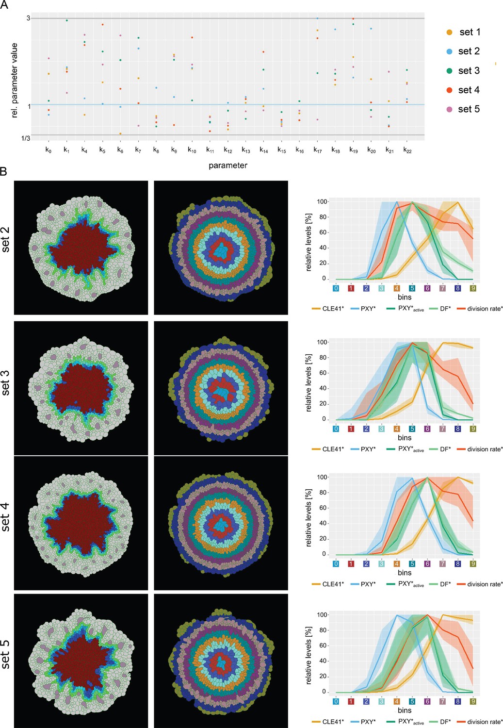
Behavior of the different model parameterizations (Model 4:2–5).
(A) Overview of parameter values of the different parameter sets. Shown are the relative values of the estimated parameter compared to the original parameter values. Horizontal lines indicate the lower (1/3) and upper (threefold) boundary (gray) as well as the original parameter value (blue). (B) Behavior of parameter sets 2–5. Shown is the final output of the simulation, the tissue* sorted into bins, as well as the average chemical concentration* per bin (for n = 10 simulations). The shading represents the range between minimal and maximal values during simulations.
Figure 5 with 4 supplements
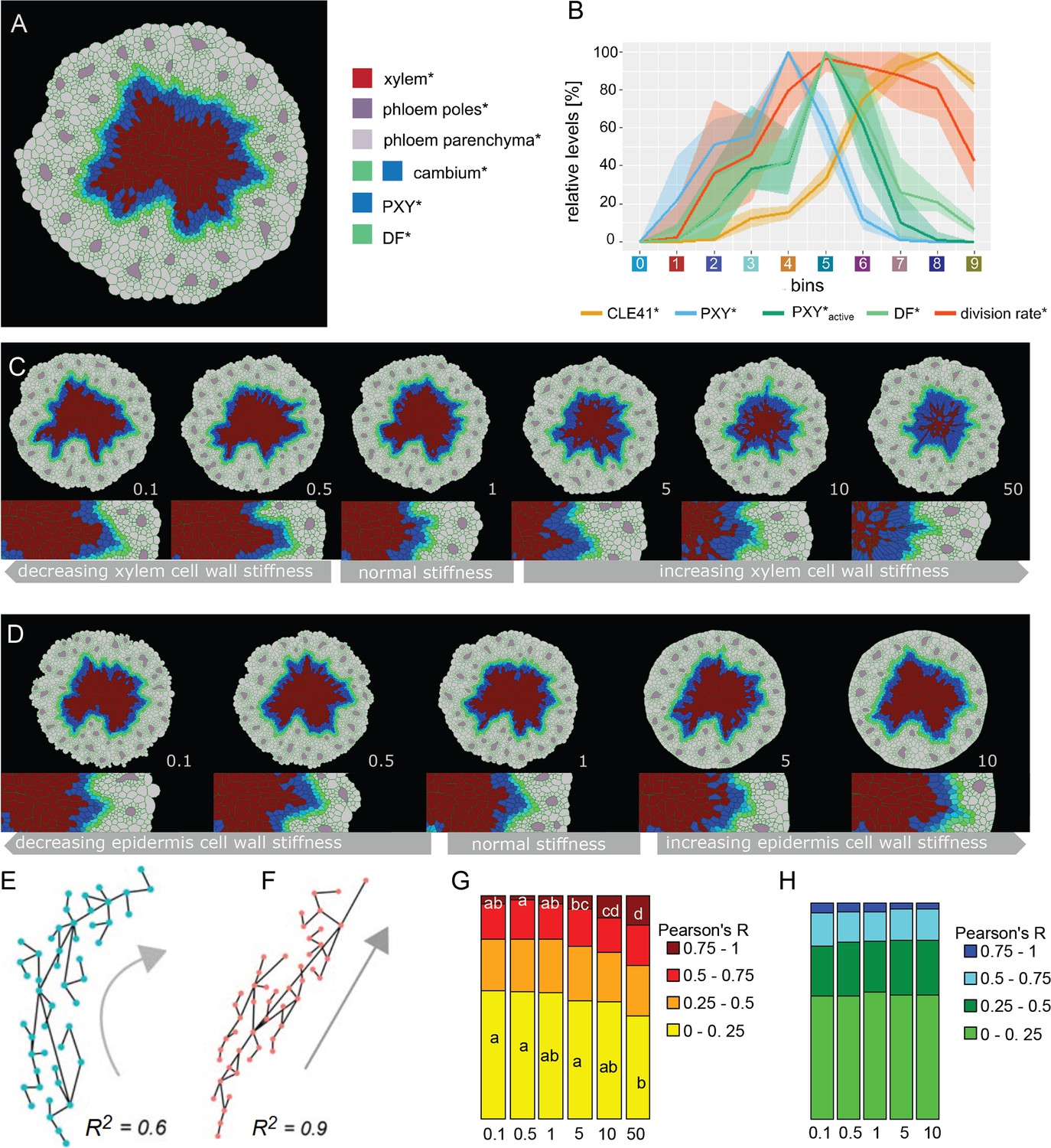
Effect of xylem cell wall stiffness* on the radiality of cambium-derived cell lineages*.
(A) Final output of Model 4 and parameter set 1. (B) Visualization of the relative levels of chemicals* and division rates* in different bins. Bin colors along the x-axis correspond to the different bins similarly as in Figure 4C. The shading represents the range between minimal and maximal values during simulations (n = 10). (C, D) Simulation outputs at increasing values of xylem stiffness* (C)and epidermis stiffness* (D)with the ratio of stiffness* vs. experimentally determined xylem stiffness indicated at the right bottom corner of each example. All the simulations had the same starting conditions and ran for the same amount of simulated time. At the bottom, there is a magnification of the right region shown in the pictures above, respectively. (E, F) Examples of the relationship between R2 and the geometry of proliferation trajectories (gray arrows) for two different R2 values; dots are cell* centroids, lines represent division* events. (G, H) Fraction of median relative amount of lineages whose R2 falls within a specific range for 30 simulations in each condition (n ≥ 70 lineages per simulation) at different xylem stiffness* (G)and epidermis stiffness* (H)regimes. In case of significant difference among medians, assessed with Kruskal–Wallis (KW significance is p<2.6 E-3 for (0, 0.25) interval and p<9.17e-7 for the (0.75,1) interval), the pairwise difference between medians was tested post hoc applying the Dunn test. The post hoc results are reported in each box as letters; medians sharing the same letter or do not display a letter at all do not differ significantly.
Figure 5—figure supplement 1
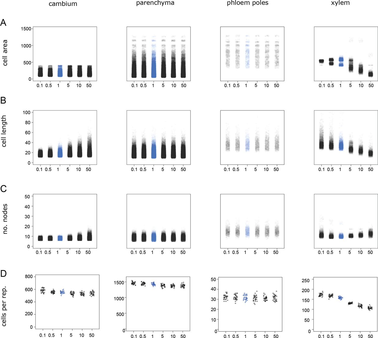
Distribution of cell* properties under different xylem ‘stiffness’ regimes.
(A) Cell* size in arbitrary units. (B) Major axis lengths of cells* in arbitrary units. (C) Numbers of nodes (vertexes) per cell*. (D) Number of cells* among cell types and stiffness values for n = 30 simulations under each stiffness regime. The blue color highlights the simulation at the experimentally determined thickness/stiffness value. The x-axis indicates values of xylem stiffness as the ratio of xylem stiffness* vs. experimentally determined thickness/stiffness. A slight horizontal displacement of points has been added to enhance visualization. Values for individual cells* found in all 30 simulations are displayed in (A–C), whereas numbers of cells* in each cell type* for each one of the 30 simulations are shown in (D).
Figure 5—figure supplement 2

Distribution of cell* properties under different tissue boundary (=epidermis*) ‘stiffness’ regimes.
(A) Cell* size in arbitrary units. (B) Major axis lengths of cells* in arbitrary units. (C) Numbers of nodes (vertexes) per cell*. (D) Number of cells* among cell types and stiffness values for n = 30 simulations under each stiffness regime. The blue color highlights the simulation running at normal stiffness level; the x-axis indicates values of the relative perimeter stiffness as the fold-change compared to the standard parameters. A slight horizontal displacement of points has been added to enhance visualization. Values for individual cells* found in all 30 simulations are displayed in (A–C), whereas numbers of cells* in each cell type* for each one of the 30 simulations are shown in (D).
Figure 5—figure supplement 3
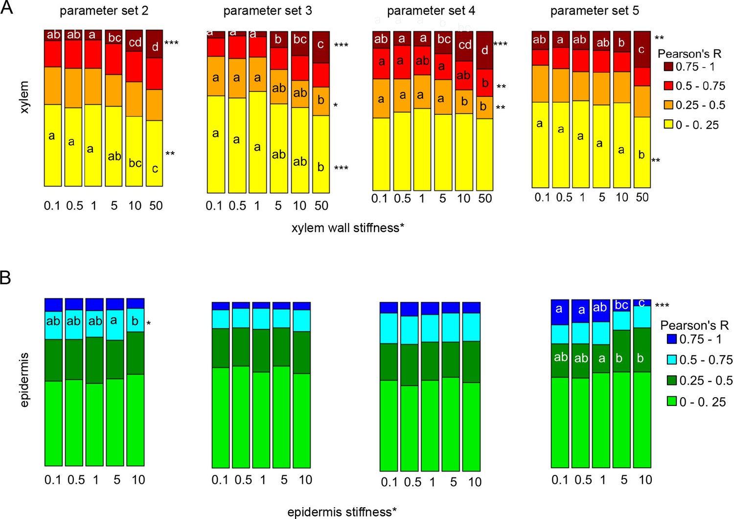
Fraction of median relative amount of cell lineages for parameter sets 2–5 for n = 30 simulations and n ≥ 60 lineages.
(A) With increasing xylem* ‘stiffness’.(B) With increasing epidermis* ‘stiffness’. KW-significance is indicated as follows: (*) p-value ≤ 0.05, (**) p-value ≤ 0.001 and (***) p value ≤ 1 E-5.
Figure 5—figure supplement 4
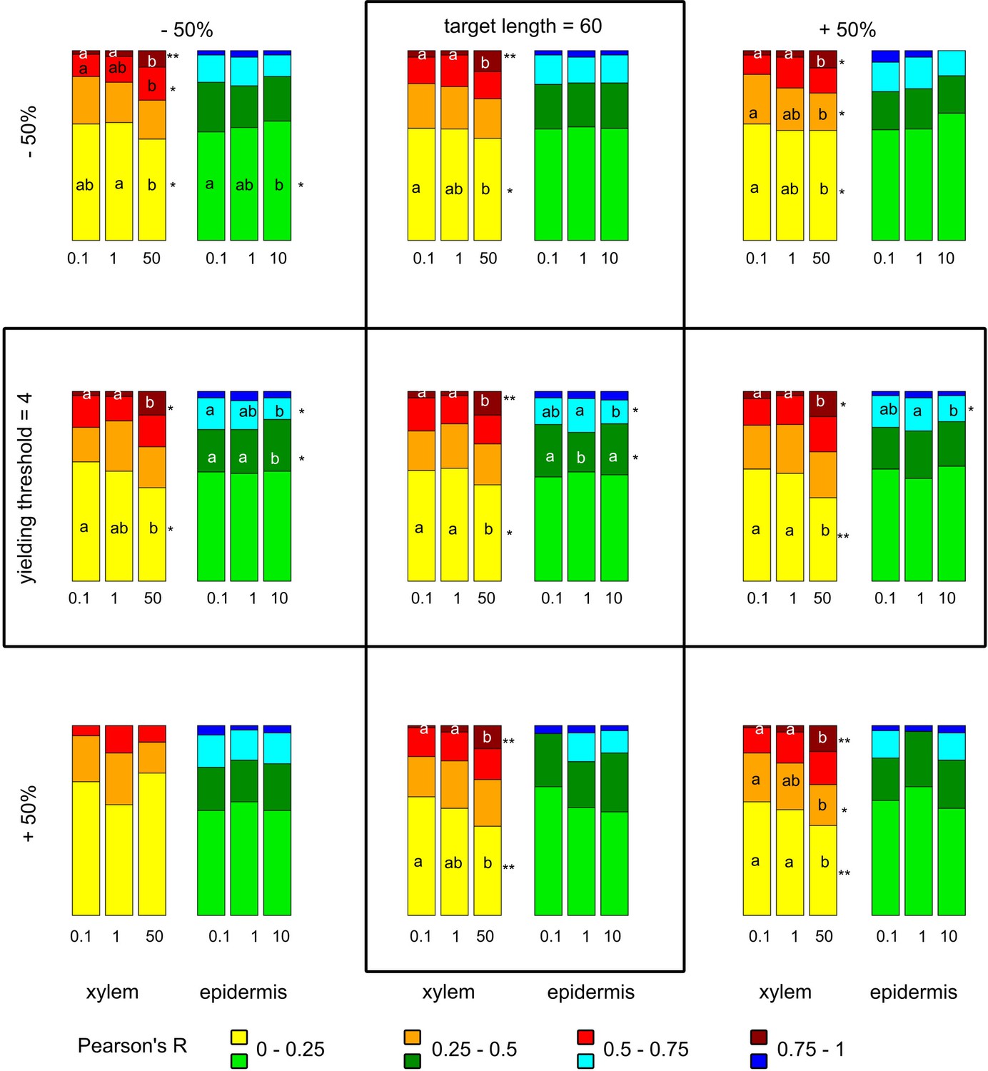
Fraction of median relative amount of cell lineages at different parameters governing cell wall* dynamics.
The model parameters cell walls’ target length and yielding threshold were varied by± 50%and the behavior at different cell wall stiffness values simulated. The statistical analysis was done as described before for Figure 5 for n = 10 simulations each and n ≥ 70cell lineages per simulation. In the case of the xylem stiffness* regime at +50% yielding threshold and - 50% target length and the epidermis* regime at +50% yielding threshold and +50% target length the sample cell lineages were insufficient for statistics. KW-significance is indicated as follows: (*) p-value ≤ 0.05, (**) p-value ≤ 0.001 and (***) p-value ≤ 1 E-5.
Appendix 1—figure 1
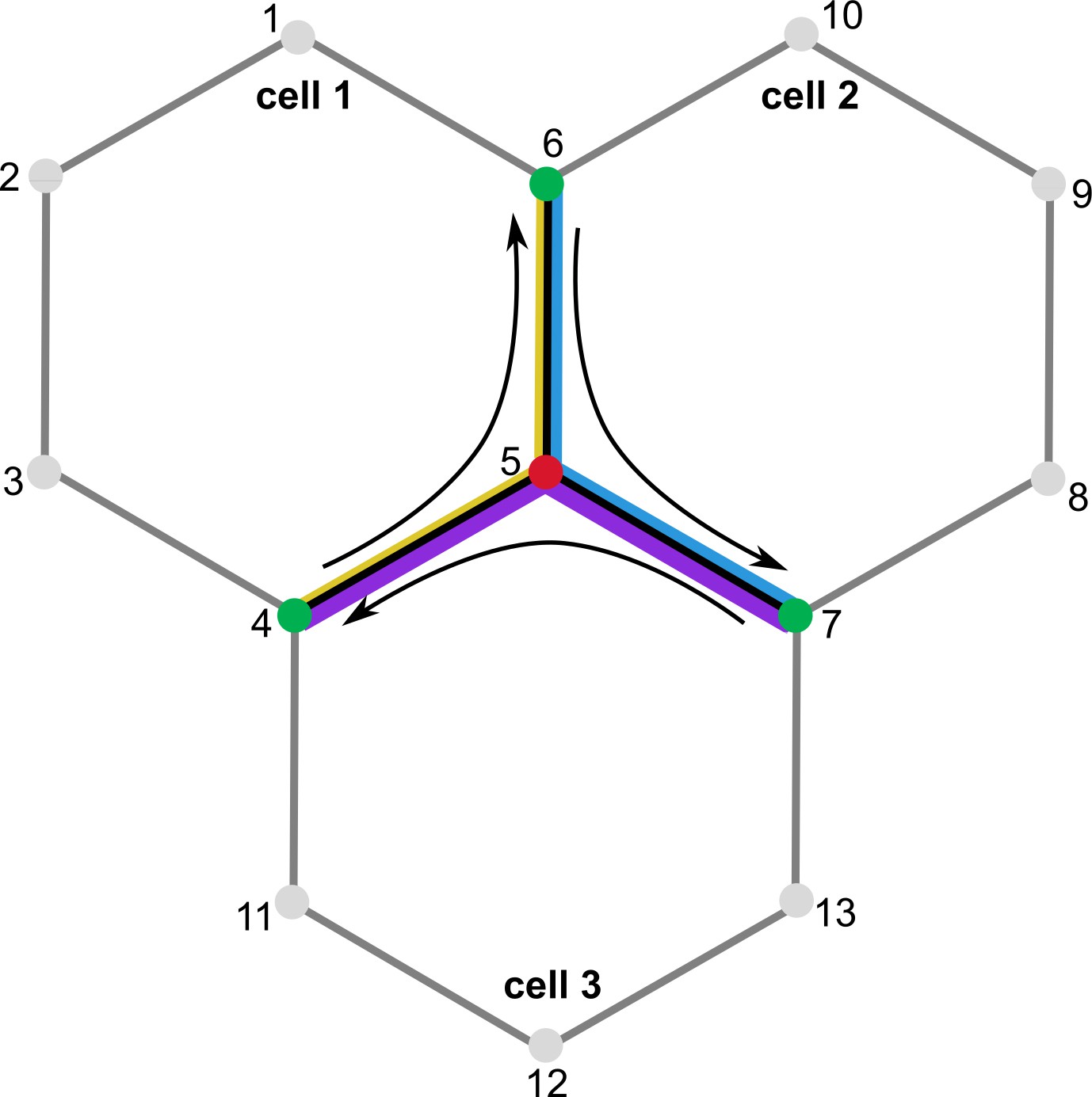
Cell wall calculations during node movement.
Node 5 is moved to a new position. During calculations, the change in wall elements between nodes 5 and 6, 5 and 7, as well as 5 and 4 is considered. The cell-specific stiffness of the wall elements is indicated by the thickness of the colored lines – yellow for cell 1, blue for cell 2, and purple for cell 3.
Videos
Video 1
Model 1 output, visualizing xylem (red) and phloem (purple), and accumulation of PXY* (blue) and PXYactive* (green).
Video 2
Model 1 output, visualizing CLE41* (yellow) accumulation.
Video 3
Model 1 output, visualizing cell divisions (red).
Video 4
Model 1 output, visualizing PXYactive*.
Video 5
Model 1 output, visualizing PXY*.
Video 6
Model 2A output, visualizing xylem (red) and phloem (purple), and accumulation of PXY* (blue) and PXY-active* (green).
Video 7
Model 2A output, visualizing CLE41* (yellow) accumulation.
Video 8
Model 2A output, visualizing cell divisions (red).
Video 9
Model 2A output, visualizing cell divisions (red) together with PXY* (blue) and PXY-active* (green) accumulation.
Video 10
Model 2A output, visualizing PXYactive*.
Video 11
Model 2A output, visualizing PXY*.
Video 12
Model 2B output, visualizing xylem (red) and phloem (purple), and accumulation of PXY* (blue), and PXY-active* (green).
Video 13
Model 2B output, visualizing CLE41* (yellow) accumulation.
Video 14
Model 2B output, visualizing cell divisions (red).
Video 15
Model 2B output, visualizing accumulation of PXY* (blue) and PXY-active* (green).
Video 16
Model 2B output, visualizing PXYactive*.
Video 17
Model 2B output, visualizing PXY*.
Video 18
Model 3A output, visualizing xylem (red), phloem parenchyma (light purple), and phloem poles (dark purple), and accumulation of PXY* (blue) and the division chemical (DF)* (green).
Video 19
Model 3A output, visualizing CLE41* (yellow) accumulation.
Video 20
Model 3A output, visualizing cell divisions (red).
Video 21
Model 3A output, visualizing accumulation of PXY* (blue) and PXYactive* (green).
Video 22
Model 3A output, visualizing PXYactive*.
Video 23
Model 3A output, visualizing PXY*.
Video 24
Model 3B output, visualizing xylem (red), phloem parenchyma (light purple), and phloem poles (dark purple), and accumulation of PXY* (blue) and the division chemical (DF)* (green).
Video 25
Model 3B output, visualizing CLE41* (yellow) accumulation.
Video 26
Model 3B output, visualizing cell divisions (red).
Video 27
Model 3B output, visualizing accumulation of PXY* (blue) and PXYactive* (green).
Video 28
Model 3B output, visualizing PXYactive*.
Video 29
Model 3B output, visualizing PXY*.
Video 30
Model 3C output, visualizing xylem (red), phloem parenchyma (light purple), and phloem poles (dark purple), and accumulation of PXY* (blue) and the division chemical (DF)* (green).
Video 31
Model 3C output, visualizing CLE41* (yellow) accumulation.
Video 32
Model 3C output, visualizing cell divisions (red).
Video 33
Model 3C output, visualizing accumulation of PXY* (blue) and the division chemical (DF)* (green).
Video 34
Model 3C output, visualizing PXYactive*.
Video 35
Model 3C output, visualizing PXY*.
Video 36
Model 4 output, parameter Set 1, visualizing xylem (red), phloem parenchyma (light purple), and phloem poles (dark purple), and accumulation of PXY* (blue) and the division chemical (DF)* (green).
Video 37
Model 4 output, parameter set 1, visualizing CLE41* (yellow) accumulation.
Video 38
Model 4 output, parameter set 1, cell divisions (red).
Video 39
Model 4 output, parameter set 1, visualizing accumulation of PXY* (blue) and the division chemical (DF)* (green).
Video 40
Model 4 output, parameter set 1, visualizing PXYactive*.
Video 41
Model 4 output, parameter set 1, visualizing PXY*.
Video 42
Model 4 output, visualizing accumulation of PXY* (blue) and the division chemical (DF)* (green) implementing a 0.1-fold change in xylem* cell wall stiffness.
Video 43
Model 4 output, visualizing accumulation of PXY* (blue) and the division chemical (DF)* (green) implementing a 0.5-fold change in xylem* cell wall stiffness.
Video 44
Model 4 output, visualizing accumulation of PXY* (blue) and the division chemical (DF)* (green) at experimentally determined xylem cell wall stiffness.
Video 45
Model 4 output, visualizing accumulation of PXY* (blue) and the division chemical (DF)* (green), implementing a 5-fold increase in xylem* cell wall stiffness.
Video 46
Model 4 output, visualizing accumulation of PXY* (blue) and the division chemical (DF)* (green), a tenfold increase in xylem* cell wall stiffness.
Video 47
Model 4 output, visualizing accumulation of PXY* (blue) and the division chemical (DF)* (green), a 50-fold increase in xylem* cell wall stiffness.
Video 48
Model 4 output, visualizing accumulation of PXY* (blue) and the division chemical (DF)* (green) implementing a 0.1-fold change in epidermis* cell wall stiffness.
Video 49
Model 4 output, visualizing accumulation of PXY* (blue) and the division chemical (DF)* (green) implementing a 0.5-fold change in epidermis* cell wall stiffness.
Video 50
Model 4 output, visualizing accumulation of PXY* (blue) and the division chemical (DF)* (green) at experimentally determined epidermis* cell wall stiffness.
Video 51
Model 4 output, visualizing accumulation of PXY* (blue) and the division chemical (DF)* (green), implementing a fivefold increase in epidermis* cell wall stiffness.
Video 52
Model 4 output, visualizing accumulation of PXY* (blue) and the division chemical (DF)* (green), a tenfold increase in epidermis* cell wall stiffness.
Additional files
-
Supplementary file 1
Table listing cell* behavior rules for Models 1–4.
- https://cdn.elifesciences.org/articles/66627/elife-66627-supp1-v2.docx
-
Supplementary file 2
Table listing parameter values and chemical thresholds after parameter estimation.
- https://cdn.elifesciences.org/articles/66627/elife-66627-supp2-v2.docx
-
Transparent reporting form
- https://cdn.elifesciences.org/articles/66627/elife-66627-transrepform1-v2.pdf
Download links
A two-part list of links to download the article, or parts of the article, in various formats.
Downloads (link to download the article as PDF)
Open citations (links to open the citations from this article in various online reference manager services)
Cite this article (links to download the citations from this article in formats compatible with various reference manager tools)
Computational modeling of cambium activity provides a regulatory framework for simulating radial plant growth
eLife 12:e66627.
https://doi.org/10.7554/eLife.66627


