Resonating neurons stabilize heterogeneous grid-cell networks
- Cellular Neurophysiology Laboratory, Molecular Biophysics Unit, Indian Institute of Science, India
Figures
Figure 1 with 1 supplement
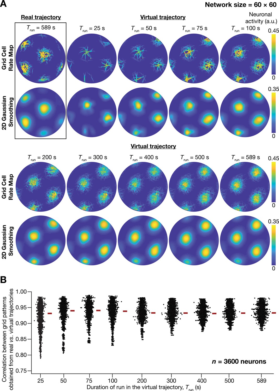
A fast virtual trajectory developed for simulating rodent run in a two-dimensional circular arena elicits grid-cell activity in a continuous attractor network (CAN) model.
(A) Panels within rectangular box: simulation of a CAN model (60 × 60 neural network) using a 589 s long real trajectory from a rat (Hafting et al., 2005) yielded grid-cell activity. Other panels: A virtual trajectory (see Materials and methods) was employed for simulating a CAN model (60 × 60 neural network) for different time points. The emergent activity patterns for nine different run times (Trun) of the virtual animal are shown to yield grid-cell activity. Top subpanels show color-coded neural activity through the trajectory, and bottom subpanels represent a smoothened spatial profile of neuronal activity shown in the respective top subpanels. (B) Pearson’s correlation coefficient between the spatial autocorrelation of rate maps using the real trajectory and the spatial autocorrelation of rate maps from the virtual trajectory for the nine different values of Trun, plotted for all neurons (n = 3600) in the network.
Figure 1—figure supplement 1
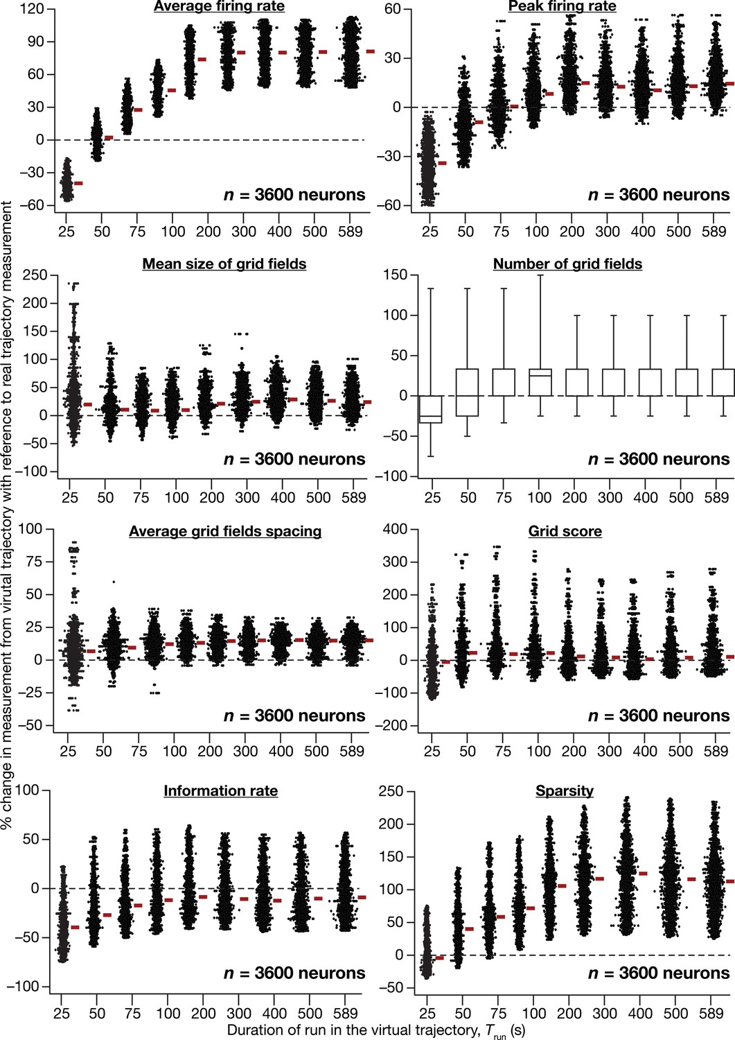
Quantitative comparison of grid-cell firing properties obtained from CAN models simulated with virtual vs. real trajectories.
Percentage changes in average firing rate, peak firing rate, mean size, number, average grid field spacing, grid score, information rate, sparsity of grid-field rate maps obtained with a virtual trajectory for the nine different values of Trun, in comparison to grid field rate maps obtained with the real trajectory (Trun = 589 s). Values are shown for all neurons (n = 3600) in the CAN model, and comparisons are made across respective neurons employing real vs. virtual trajectories.
Figure 2
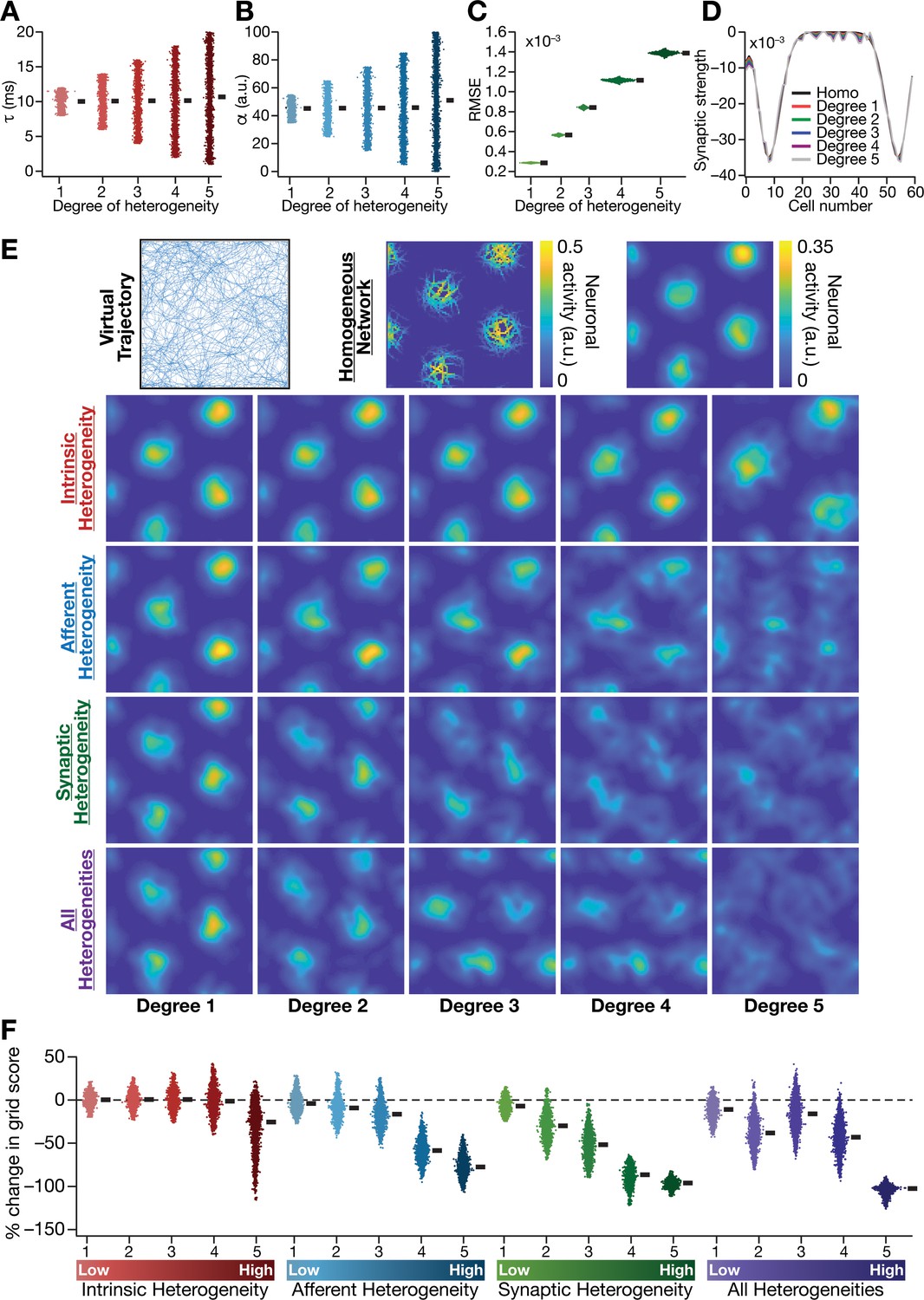
Biologically prevalent network heterogeneities disrupt the emergence of grid-cell activity in CAN models.
(A) Intrinsic heterogeneity was introduced by setting the integration time constant () of each neuron to a random value picked from a uniform distribution, whose range was increased to enhance the degree of intrinsic heterogeneity. The values of for the 3600 neurons in the 60 × 60 CAN model are shown for 5 degrees of intrinsic heterogeneity. (B) Afferent heterogeneity was introduced by setting the velocity-scaling factor () of each neuron to a random value picked from a uniform distribution, whose range was increased to enhance the degree of intrinsic heterogeneity. The values of for the 3600 neurons are shown for 5 degrees of afferent heterogeneity. (C) Synaptic heterogeneity was introduced as an additive jitter to the intra-network Mexican hat connectivity matrix, with the magnitude of additive jitter defining the degree of synaptic heterogeneity. Plotted are the root mean square error (RMSE) values computed between the connectivity matrix of ‘no jitter’ case and that for different degrees of synaptic heterogeneities, across all synapses. (D) Illustration of a one-dimensional slice of synaptic strengths with different degrees of heterogeneity, depicted for Mexican-hat connectivity of a given cell to 60 other cells in the network. (E) Top left, virtual trajectory employed to obtain activity patterns of the CAN model. Top center, Example rate maps of grid-cell activity in a homogeneous CAN model. Top right, smoothed version of the rate map. Rows 2–4: smoothed version of rate maps obtained from CAN models endowed with five different degrees (increasing left to right) of disparate forms (Row 2: intrinsic; Row 3: afferent; Row 4: synaptic; and Row 5: all three heterogeneities together) of heterogeneities. (F) Percentage change in the grid score of individual neurons (n = 3600) in networks endowed with the four forms and five degrees of heterogeneities, compared to the grid score of respective neurons in the homogeneous network.
Figure 3 with 3 supplements
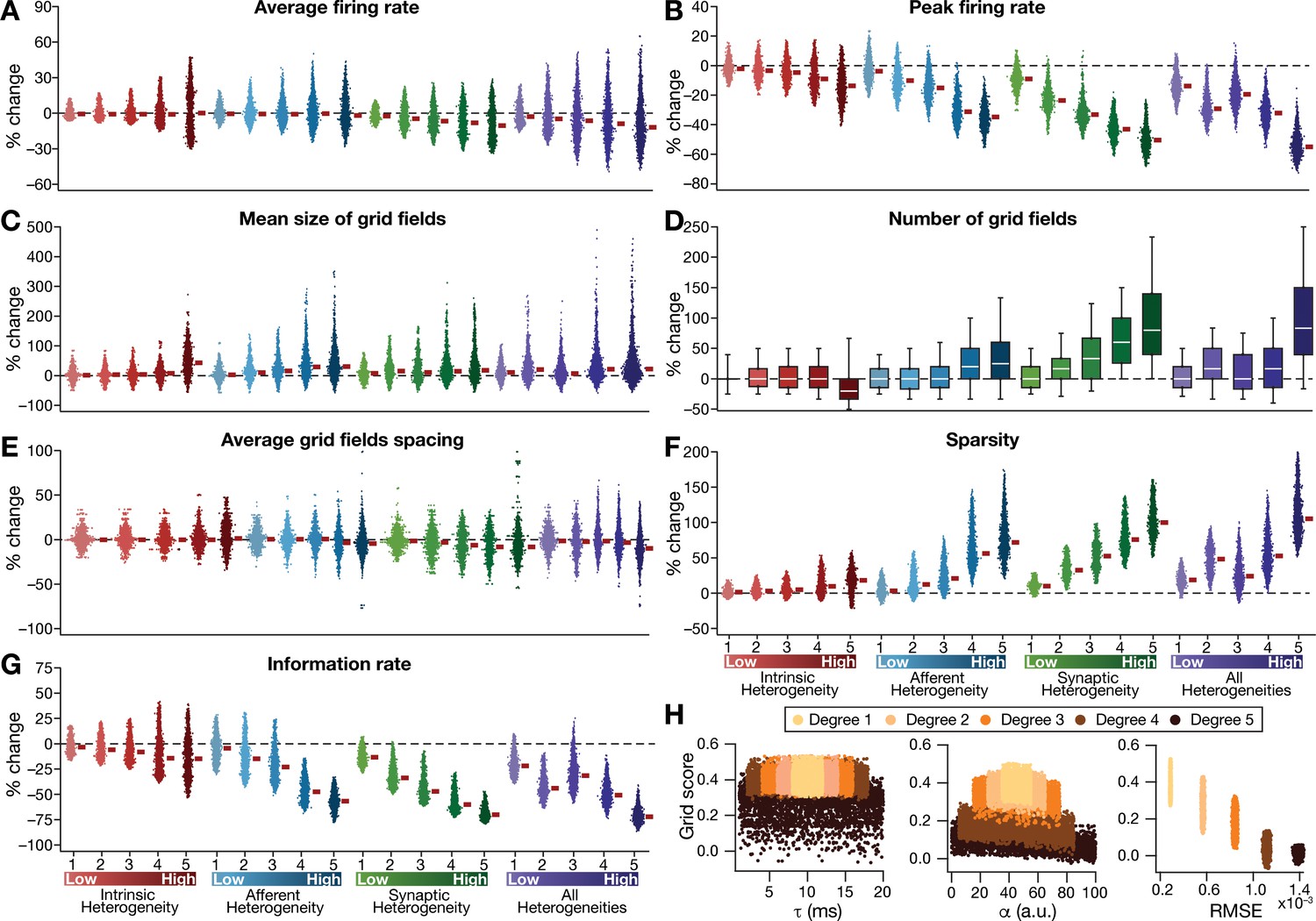
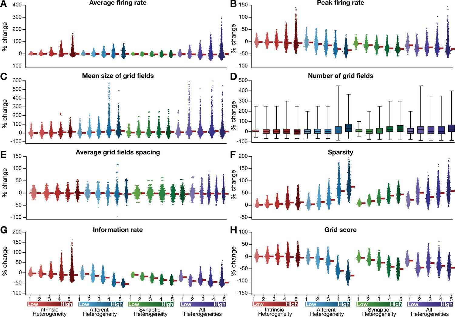
Quantification of the disruption in grid-cell activity induced by different forms of network heterogeneities in the CAN model.
Grid-cell activity of individual neurons in the network was quantified by eight different measurements, for CAN models endowed independently with intrinsic, afferent, or synaptic heterogeneities or a combination of all three heterogeneities. (A–G) Depicted are percentage changes in each of average firing rate (A), peak firing rate (B), mean size (C), number (D), average spacing (E), information rate (F), and sparsity (G) for individual neurons (n = 3600) in networks endowed with distinct forms of heterogeneities, compared to the grid score of respective neurons in the homogeneous network. (H) Grid score of individual cells (n = 3600) in the network plotted as functions of integration time constant (), velocity modulation factor (), and root mean square error (RMSE) between the connectivity matrices of the homogeneous and the heterogeneous CAN models. Different colors specify different degrees of heterogeneity. The three plots with reference to , , and RMSE are from networks endowed with intrinsic, afferent, and synaptic heterogeneity, respectively.
Figure 3—figure supplement 1
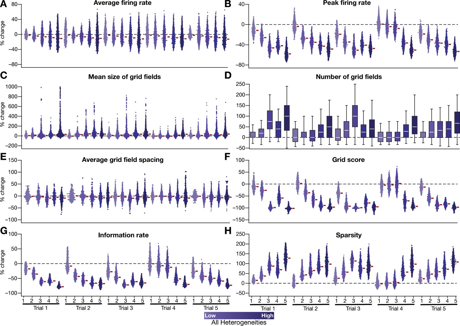
Quantification of the disruption of grid-cell firing by network heterogeneities across different trials of CAN-model simulations.
(A–H) Grid-cell activity of individual neurons in the network was quantified by eight different measurements from five sets of trials (excluding the trial shown and quantified in Figures 2–3). Distinct trials are obtained by unique initialization of the continuous attractor network and independent randomization of parametric values in introducing network heterogeneities. Depicted are percentage changes in each measurement of individual neurons (n = 3600) in networks endowed with 5 degrees of heterogeneities, compared to the grid maps of respective neurons in the homogeneous network. All simulations in this figure are endowed with all the three forms (intrinsic, afferent, and synaptic) of heterogeneities.
Figure 3—figure supplement 2
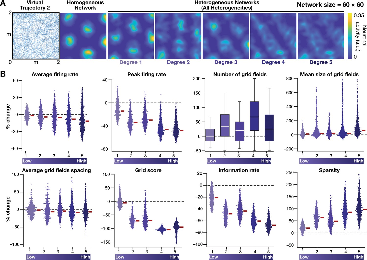
Disruption of grid-cell firing by network heterogeneities was invariant to the specific trajectory employed by the CAN models.
(A) Left to right: Virtual trajectory in a square arena (dimensions: 2 m × 2 m), which is distinct from that shown in Figure 2E, was employed to perform CAN model simulations reported in this figure. Example rate map of grid-cell activity in a homogeneous network, and in heterogeneous networks endowed with 5 degrees of heterogeneities, obtained with ‘Virtual trajectory 2’. (B) Percentage changes in grid-cell measurements from heterogeneous CAN models with reference to those in homogeneous CAN model measurements for all neurons in the network (n = 3600), obtained with ‘Virtual trajectory 2’. All simulations in this figure are endowed with all the three forms (intrinsic, afferent, and synaptic) of heterogeneities.
Figure 3—figure supplement 3
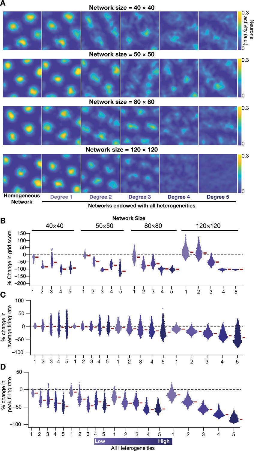
Disruption of grid-cell activity by network heterogeneities was prevalent across CAN models of different sizes.
(A) Example rate maps of grid-cell activity for homogeneous (Column 1) and heterogeneous networks endowed with five different degrees of heterogeneities (Columns 2–6) for networks of different sizes (Row 1: 40 × 40; Row 2: 50 × 50; Row 3: 80 × 80; Row 4: 120 × 120). (B) Percentage change in the grid score of individual neurons in networks of different sizes, endowed with five degrees of heterogeneities, compared to the grid score of neurons in homogeneous networks of respective sizes. Percent changes in average (C) and peak (D) firing rate of grid-cell activity for individual neurons in heterogeneous network with different degrees of heterogeneity, computed with reference to the values from their respective homogeneous network. All simulations in this figure are endowed with all the three forms (intrinsic, afferent, and synaptic) of heterogeneities.
Figure 4
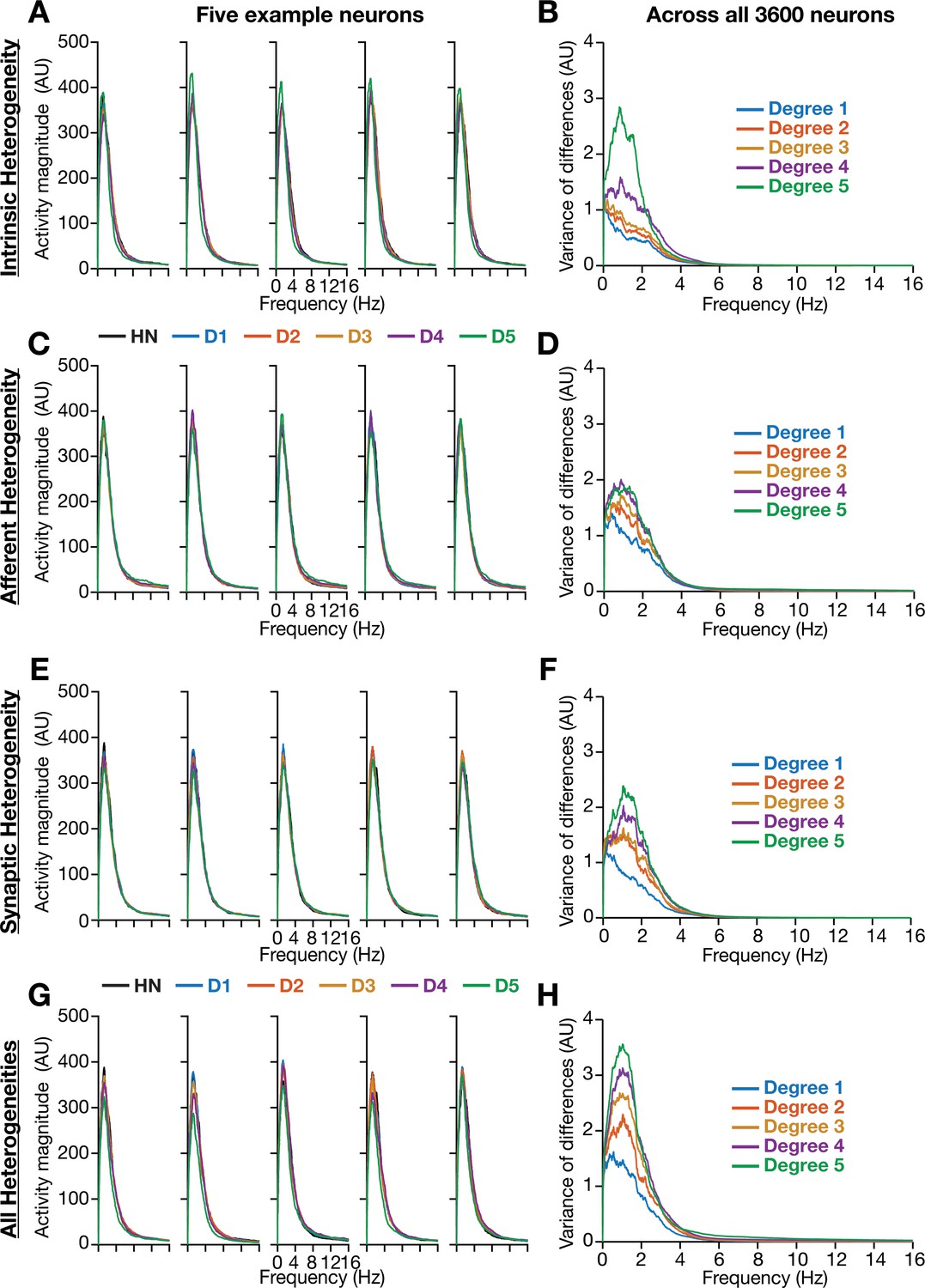
Incorporation of biological heterogeneities predominantly altered neural activity in low frequencies.
(A–H) Left, Magnitude spectra of temporal activity patterns of five example neurons residing in a homogeneous network (HN) or in networks with different forms and degrees of heterogeneities. Right, Normalized variance of the differences between the magnitude spectra of temporal activity of neurons in homogeneous vs. heterogeneous networks, across different forms and degrees of heterogeneities, plotted as a function of frequency.
Figure 5
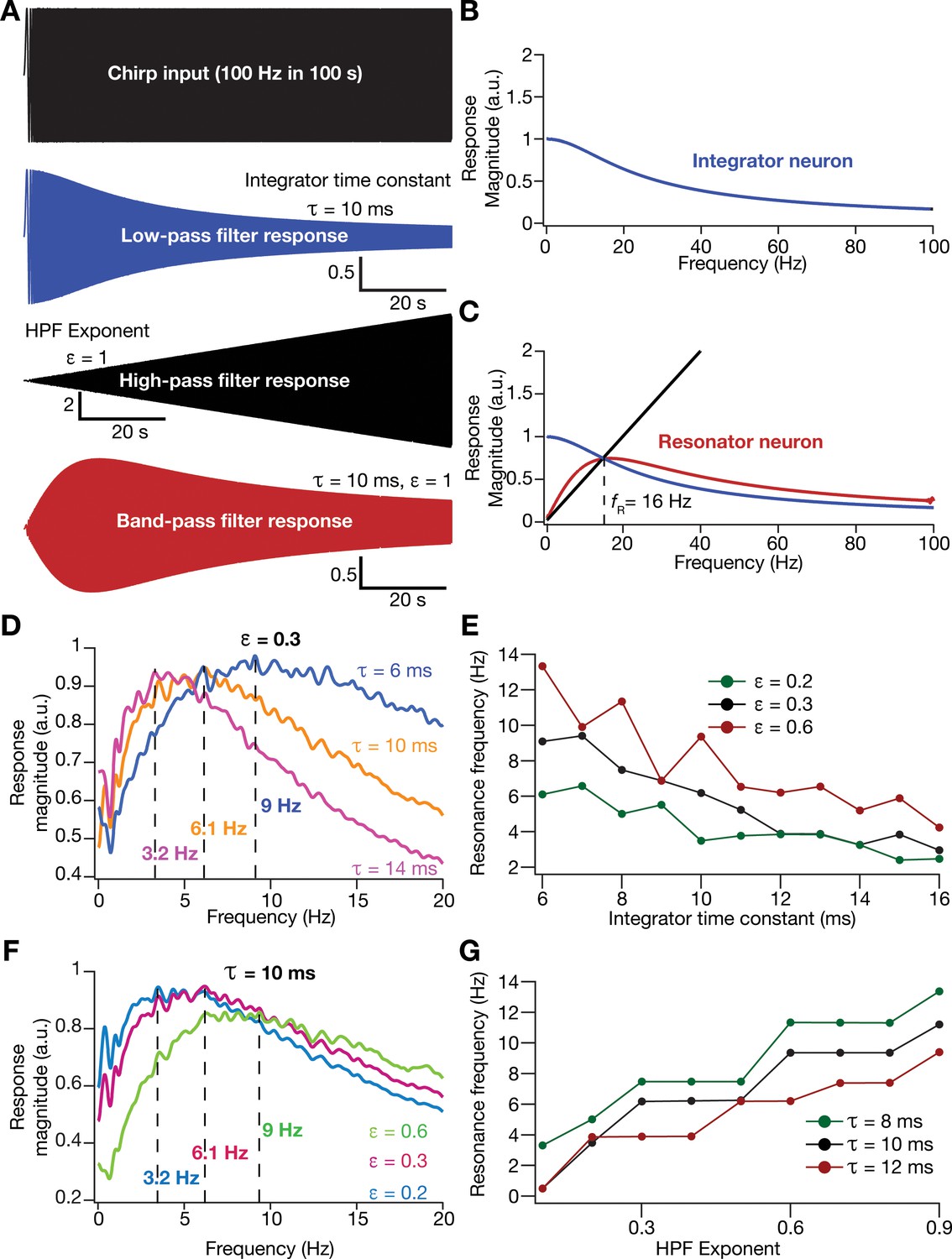
Incorporation of an additional high-pass filter into neuronal dynamics introduces resonance in individual rate-based neurons.
(A) Responses of neurons with low-pass (integrator; blue), high-pass (black) and band-pass (resonator; red) filtering structures to a chirp stimulus (top). Equations (7–8) were employed for computing these responses. (B) Response magnitude of an integrator neuron (low-pass filter) as a function of input frequency, derived from response to the chirp stimulus. (C) Response magnitude of a resonator neuron (band-pass filter; red) as a function of input frequency, derived from response to the chirp stimulus, shown to emerge as a combination of low- (blue) and high-pass (black) filters. represents resonance frequency. The response magnitudes in (B, C) were derived from respective color-coded traces shown in (A). (D–E) Tuning resonance frequency by altering the low-pass filter characteristics. Response magnitudes of three different resonating neurons with identical HPF exponent ( = 0.3), but with different integrator time constants (), plotted as functions of frequency (D). Resonance frequency can be tuned by adjusting for different fixed values of , with an increase in yielding a reduction in (E). (F–G) Tuning resonance frequency by altering the high-pass filter characteristics. Response magnitudes of three different resonating neurons with identical (=10 ms), but with different values for , plotted as functions of frequency (F). Resonance frequency can be tuned by adjusting for different fixed values of , with an increase in yielding an increase in (G).
Figure 6 with 1 supplement

Impact of neuronal resonance, introduced by altering low-pass filter characteristics, on grid-cell activity in a homogeneous CAN model.
(A) Example rate maps of grid-cell activity from a homogeneous CAN model with integrator neurons modeled with different values for integration time constants (). (B) Example rate maps of grid-cell activity from a homogeneous CAN model with resonator neurons modeled with different values. (C–F) Grid score (C), average spacing (D), mean size (E), and number (F) of grid fields in the arena for all neurons (n = 3600) in homogeneous CAN models with integrator (blue) or resonator (red) neurons, modeled with different values. The HPF exponent was set to 0.3 for all resonator neuronal models.
Figure 6—figure supplement 1
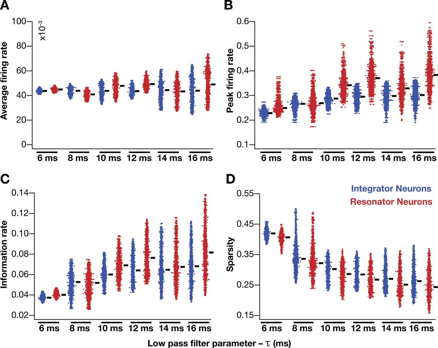
Impact of neuronal resonance (phenomenological model), introduced by altering low-pass filter characteristics, on grid-cell characteristics in a homogeneous CAN model.
(A–D) average firing rate (A), peak firing rate (B), information rate (C), and sparsity (D) of grid fields in the arena for all neurons (n = 3600) in homogeneous CAN models with integrator (blue) or resonator (red) neurons, modeled with different 𝜏 values. The HPF exponent ε was set to 0.3 for all resonator neuronal models.
Figure 7
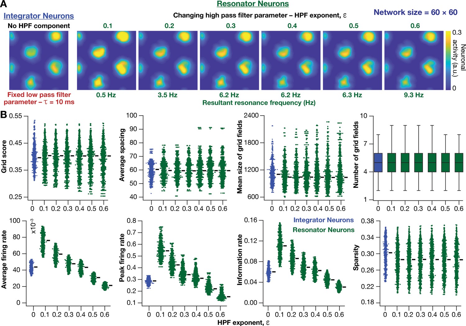
Impact of neuronal resonance, introduced by altering high-pass filter characteristics, on grid-cell activity in a homogeneous CAN model.
(A) Example rate maps of grid-cell activity from a homogeneous CAN model with integrator neurons (Column 1) or resonator neurons (Columns 2–6) modeled with different values of the HPF exponent (). (B) Comparing 8 metrics of grid-cell activity for all the neurons (n = 3600) in CAN models with integrator (blue) or resonator (green) neurons. CAN models with resonator neurons were simulated for different values. = 10 ms for all networks depicted in this figure.
Figure 8 with 2 supplements
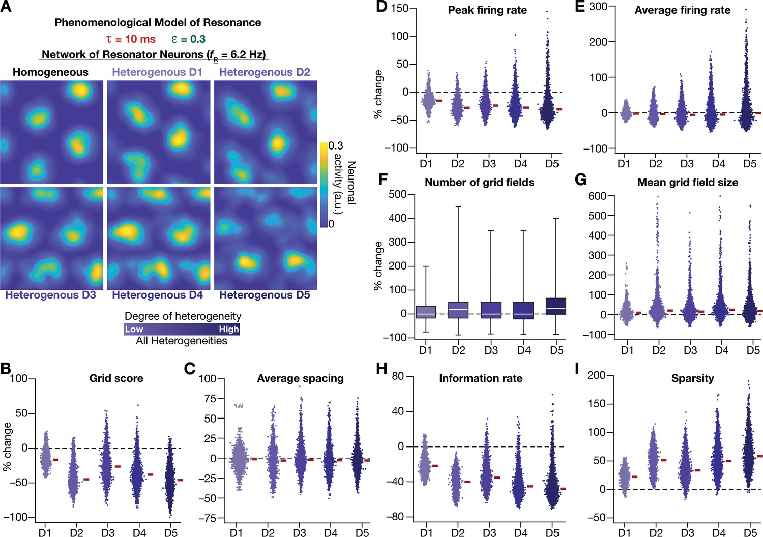
Neuronal resonance stabilizes grid-cell activity in heterogeneous CAN models.
(A) Example rate maps of grid-cell activity in homogeneous (Top left) and heterogeneous CAN models, endowed with resonating neurons, across different degrees of heterogeneities. (B–I) Percentage changes in grid score (B), average spacing (C), peak firing rate (D), average firing rate (E), number (F), mean size (G), information rate (H), and sparsity (I) of grid field for all neurons (n = 3600) in the heterogeneous CAN model, plotted for 5 degrees of heterogeneities (D1–D5), compared with respective neurons in the homogeneous resonator network. All three forms of heterogeneities were incorporated together into the network. = 0.3 and = 10 ms for all networks depicted in this figure.
Figure 8—figure supplement 1
Quantification of the grid-cell activity in presence of different forms of network heterogeneities in the CAN model with phenomenological resonator neurons.
Grid cell activity of individual resonator neurons in the network was quantified by eight different measurements, for CAN models endowed independently with intrinsic, afferent, or synaptic heterogeneities or a combination of all three heterogeneities. (A–H) Depicted are percentage changes in each of average firing rate (A), peak firing rate (B), mean size (C), number (D), average spacing (E), information rate (F), sparsity (G), and grid score (H) for individual neurons (n = 3600) in networks endowed with distinct forms of heterogeneities, compared to the grid score of respective neurons in the homogeneous network.
Figure 8—figure supplement 2
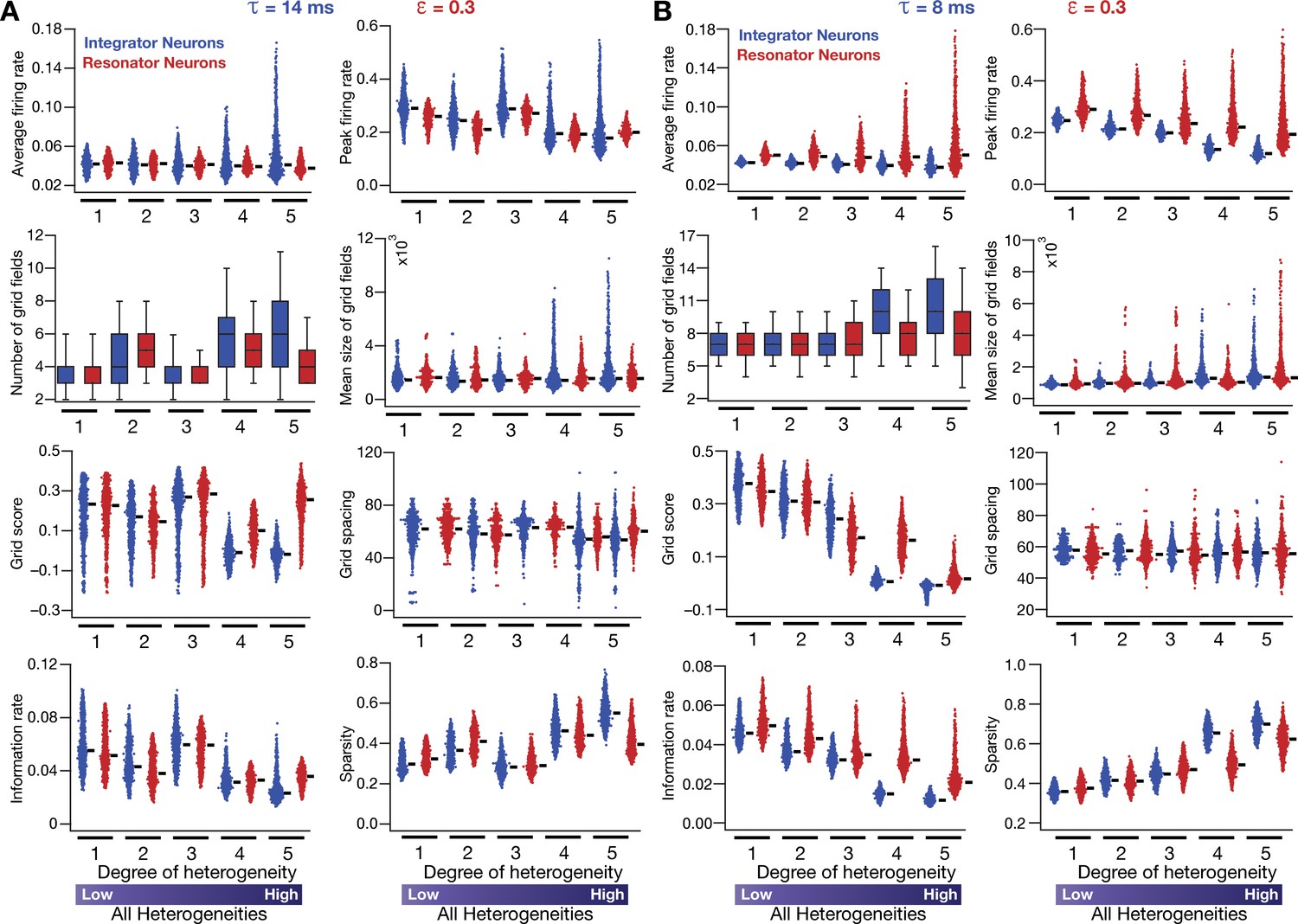
Neuronal resonance (phenomenological) stabilizes grid-cell firing in heterogeneous CAN models.
(A) Average firing rate, peak firing rate, mean size, number, average grid field spacing, grid score, information rate, and sparsity of grid fields for all neurons (n = 3600) in heterogeneous CAN models with integrator (blue) or resonator (red) neurons, shown across 5 degrees of heterogeneities. All neurons in all networks were endowed with an integration time constant = 14 ms, and all resonator neurons were built with HPF exponent value = 0.3. (B) Same as (A), but with = 8 ms for all neurons. All simulations in this figure are endowed with all the three forms (intrinsic, afferent, and synaptic) of heterogeneities. In imposing intrinsic heterogeneities, the span of the uniform distributions that governed was always centered at the respective values (= 14 ms for A and = 8 ms for B), with the extent of the uniform distribution increasing with increased degree of heterogeneity.
Figure 9
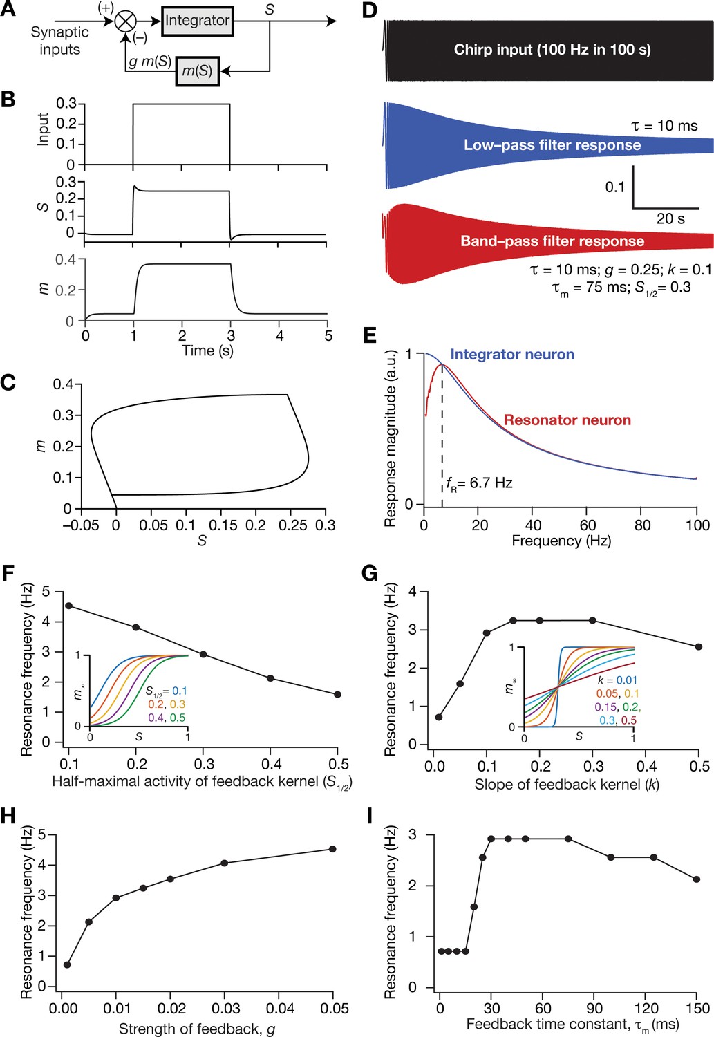
Incorporation of a slow negative feedback loop into single-neuron dynamics introduces tunable resonance in rate-based neuronal models.
(A) A mechanistic model of intrinsic resonance in individual neurons using a slow negative feedback loop. (B) Temporal evolution of the output () of an individual neuron and the state variable related to the negative feedback () in response for square pulse. (C) Phase-plane representation of the dynamics depicted in (B). (D) Responses of neurons with low-pass (integrator; blue) and band-pass (resonator; red) filtering structures to a chirp stimulus (top). The resonator was implemented through the introduction of a slow negative feedback loop (A). Equations (10–12) were employed for computing these responses. (E) Response magnitude of an integrator neuron (low-pass filter, blue) and resonator neuron (band-pass filter, red) as functions of input frequency, derived from their respective responses to the chirp stimulus. represents resonance frequency. The response magnitudes in (E) was derived from respective color-coded traces shown in (D). (F–I) Tuning resonance frequency by altering the parameters of the slow negative feedback loop. Resonance frequency, obtained from an individual resonator neuron responding to a chirp stimulus, is plotted as functions of half maximal activity of the feedback kernel, (F), slope of the feedback kernel, (G), strength of negative feedback, (H), and feedback time constant, (I). The insets in (F) and (G) depict the impact of altering and on the feedback kernel (), respectively.
Figure 10 with 2 supplements
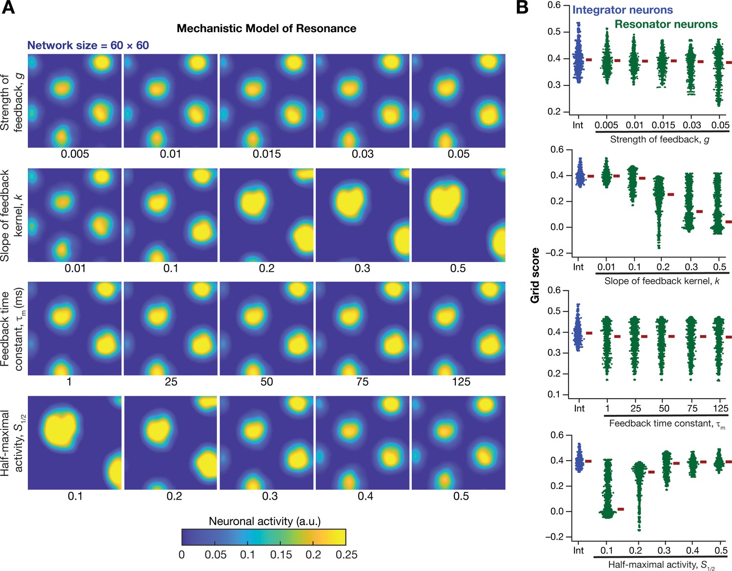
Impact of neuronal resonance, introduced by a slow negative feedback loop, on grid-cell activity in a homogeneous CAN model.
(A) Example rate maps of grid-cell activity from a homogeneous CAN model for different values of the feedback strength () slope of the feedback kernel (), feedback time constant (), and half maximal activity of the feedback kernel, . (B) Grid scores for all the neurons in the homogeneous CAN model for different values of , , , and in resonator neurons (green). Grid scores for homogeneous CAN models with integrator neurons (without the negative feedback loop) are also shown (blue). Note that although pattern neural activity is observed across all networks, the grid score is lower in some cases because of the large size and lower numbers of grid fields within the arena with those parametric configurations.
Figure 10—figure supplement 1
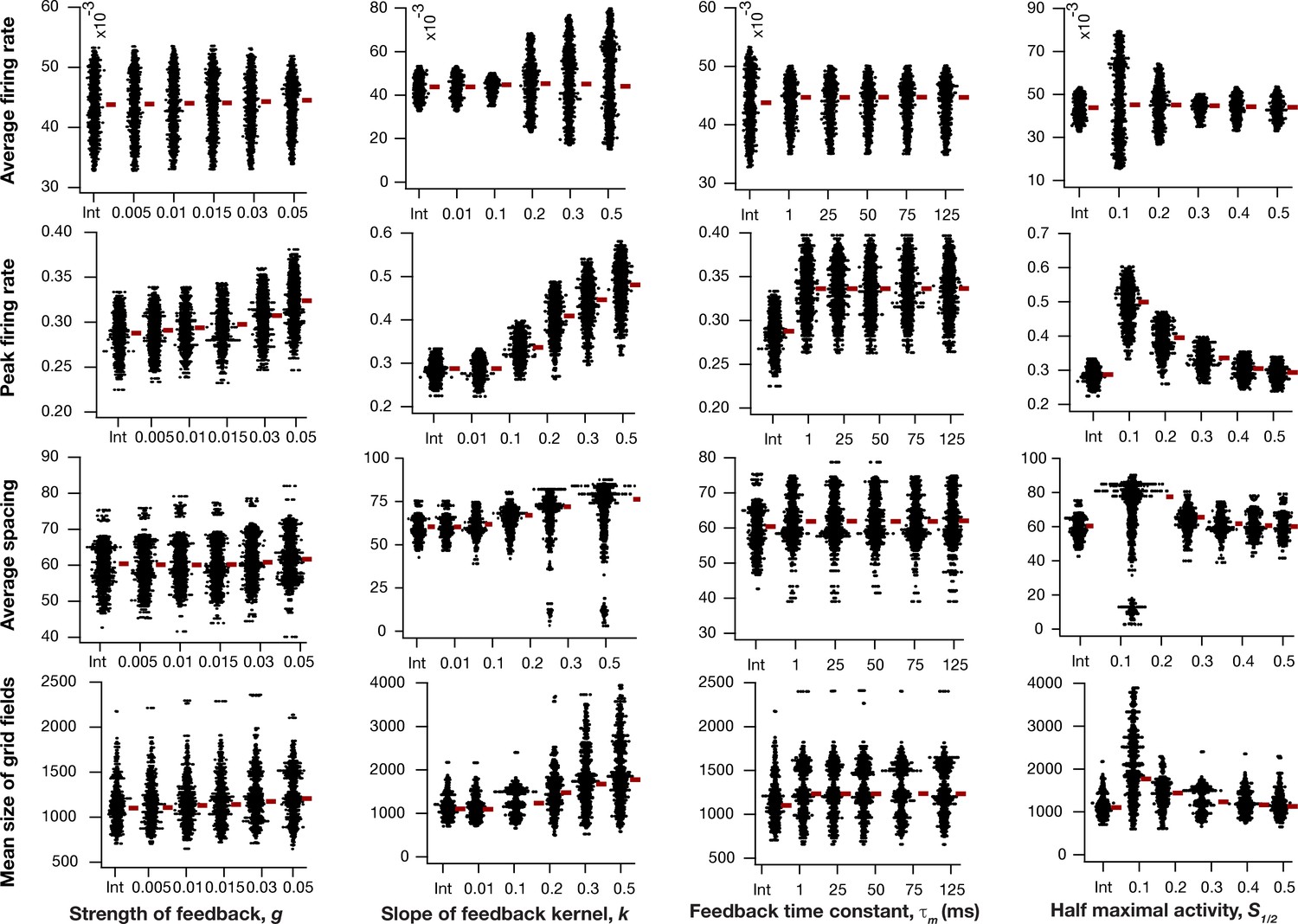
Impact of intrinsic neuronal resonance, introduced by adding a negative feedback loop in the neuronal dynamics, on grid-cell characteristics in a homogeneous CAN model.
Average firing rate (Row 1), peak firing rate (Row 2), average spacing (Row 3), and mean size (Row 4) of grid fields in the arena for all neurons (n = 3600) in homogeneous CAN models and their dependence on the parameters of negative feedback loop (, , , and ) compared to homogeneous CAN model with integrator neurons (Int). Please note that the parameters were adjusted such that average firing rate in maintained at similar level across different parametric values.
Figure 10—figure supplement 2
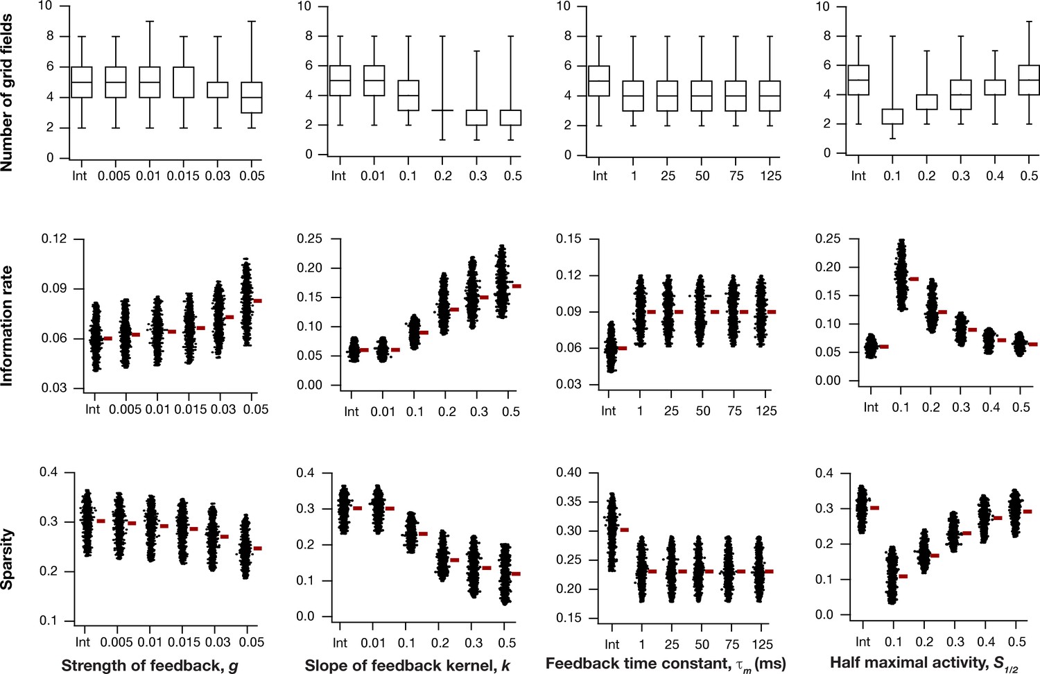
Impact of intrinsic neuronal resonance, introduced by adding a negative feedback loop in the neuronal dynamics, on grid-cell characteristics in a homogeneous CAN model.
Number (Row 1), information rate (Row 2), and sparsity (Row 3) of grid fields in the arena for all neurons (n = 3600) in homogeneous CAN models and their dependence on the parameters of negative feedback loop (, , , and ) compared to homogeneous CAN model with integrator neurons (Int).
Figure 11 with 1 supplement
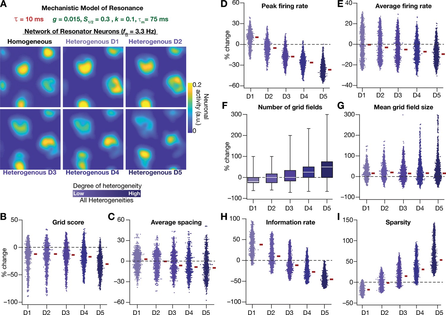
Resonating neurons, achieved through a slow negative feedback loop, stabilizes grid-cell activity in heterogeneous CAN models.
(A) Example rate maps of grid-cell activity in homogeneous (top left) and heterogeneous CAN models, endowed with resonating neurons, across different degrees of heterogeneities. (B–I) Percentage changes in grid score (B), average spacing (C), peak firing rate (D), average firing rate (E), number (F), mean size (G), information rate (H), and sparsity (I) of grid field for all neurons (n = 3600) in the heterogeneous CAN model, plotted for 5 degrees of heterogeneities (D1–D5). The percentage changes are computed with reference to respective neurons in the homogeneous resonator network. All three forms of heterogeneities were incorporated together into these networks.
Figure 11—figure supplement 1
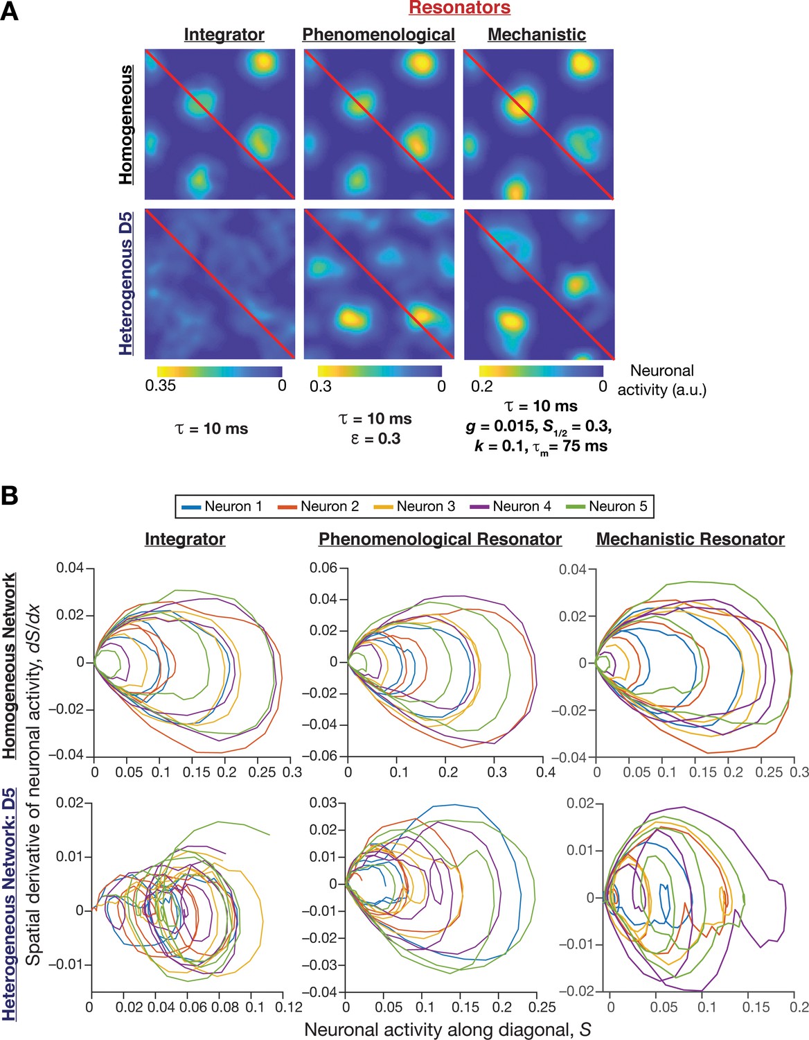
Phase plane analysis of spatial profiles provided visualizations of the disruption of grid-cell activity in heterogeneous integrator networks and the relative robustness of heterogeneous resonator networks.
(A) Example rate maps of grid-cell activity in homogeneous (Row 1) and heterogeneous (Row 2; all heterogeneities, degree 5) CAN models, endowed with integrator (Column 1) or phenomenological resonator (Column 2) or mechanistic resonator (Column 3) neurons. Maps in Columns 1–3 are from Figure 2E, Figure 8A, and Figure 11A, respectively. The diagonal values of these spatial rate maps (red lines) were employed for phase plane analysis. The choice of the diagonal was driven by the need to maximize the number of spatial activity cycles. (B) Phase-plane plots showing neuronal activity along the diagonal plotted against its spatial derivative for five different neurons in homogeneous (Row 1) and heterogeneous (Row 2; all heterogeneities, degree 5) CAN models, endowed with integrator (Column 1) or phenomenological resonator (Row 2) or mechanistic resonator (Row 3) neurons. Note the manifestation of closed orbits in homogeneous networks, the complete loss of closed orbits in the heterogeneous integrator network and the presence of noisy closed orbits in the heterogeneous resonator networks.
Figure 12
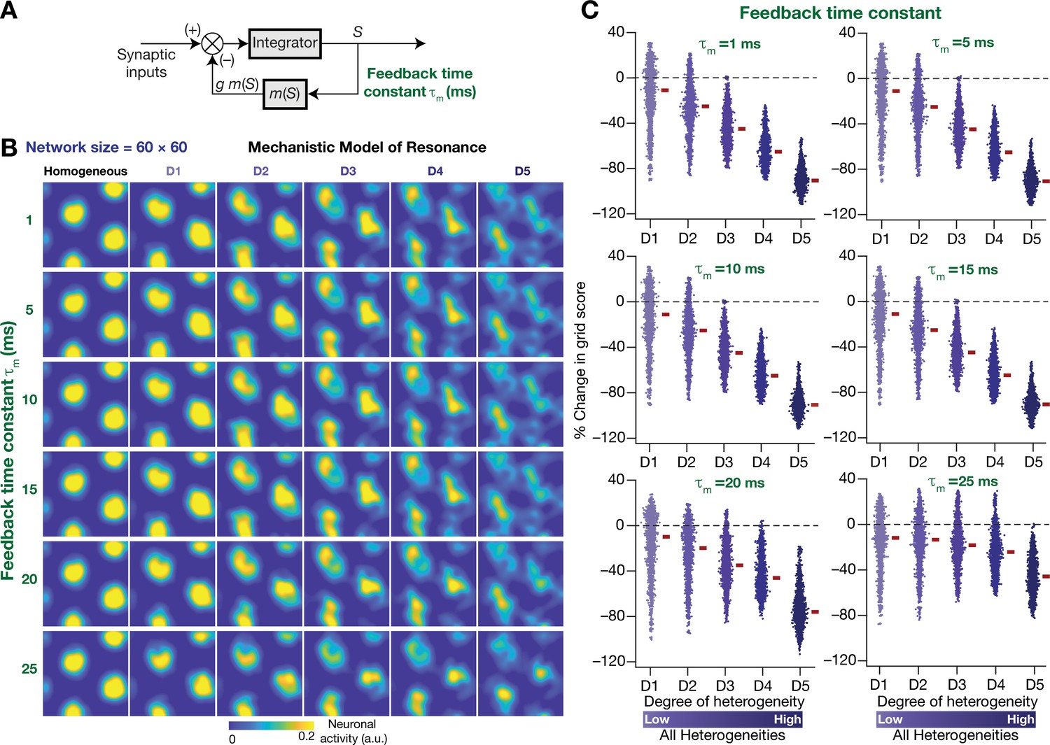
The slow kinetics of the negative feedback loop is a critical requirement for stabilizing heterogeneous CAN models.
(A) A mechanistic model of intrinsic resonance in individual neurons using a slow negative feedback loop, with the feedback time constant () defining the slow kinetics. (B) Example rate maps of grid-cell activity in homogeneous (top left) and heterogeneous CAN models, endowed with neurons built with different values of , across different degrees of heterogeneities. (C) Percentage changes in grid score for all neurons (n = 3600) in the heterogeneous CAN model, endowed with neurons built with different values of , plotted for 5 degrees of heterogeneities (D1–D5). The percentage changes are computed with reference to respective neurons in the homogeneous resonator network. All three forms of heterogeneities were incorporated together into these networks.
Figure 13 with 3 supplements
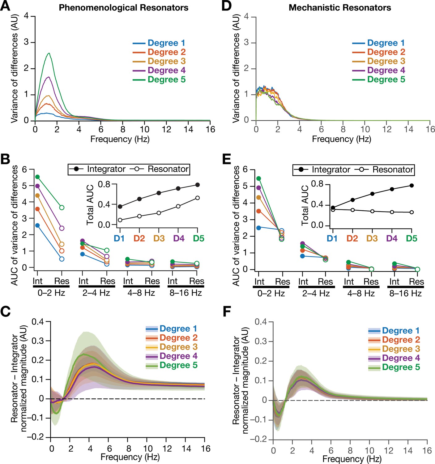
Intrinsically resonating neurons suppressed heterogeneity-induced variability in low-frequency perturbations caused by the incorporation of biological heterogeneities.
(A) Normalized variance of the differences between the magnitude spectra of temporal activity in neurons of homogeneous vs. heterogeneous networks, across different degrees of all three forms of heterogeneities expressed together, plotted as a function of frequency. (B) Area under the curve (AUC) of the normalized variance plots shown in Figure 4H (for the integrator network) and (A) (for the phenomenological resonator network) showing the variance to be lower in resonator networks compared to integrator networks. The inset shows the total AUC across all frequencies for the integrator vs. the resonator networks as a function of the degree of heterogeneities. (C) Difference between the normalized magnitude spectra of neural temporal activity patterns for integrator and resonator neurons in CAN models. Solid lines depict the mean and shaded area depicts the standard deviations, across all 3600 neurons. The resonator networks in (A–C) were built with phenomenological resonators. (D–F) same as (A–C) but for the mechanistic model of intrinsic resonance. All heterogeneities were simultaneously expressed for all the analyses presented in this figure.
Figure 13—figure supplement 1
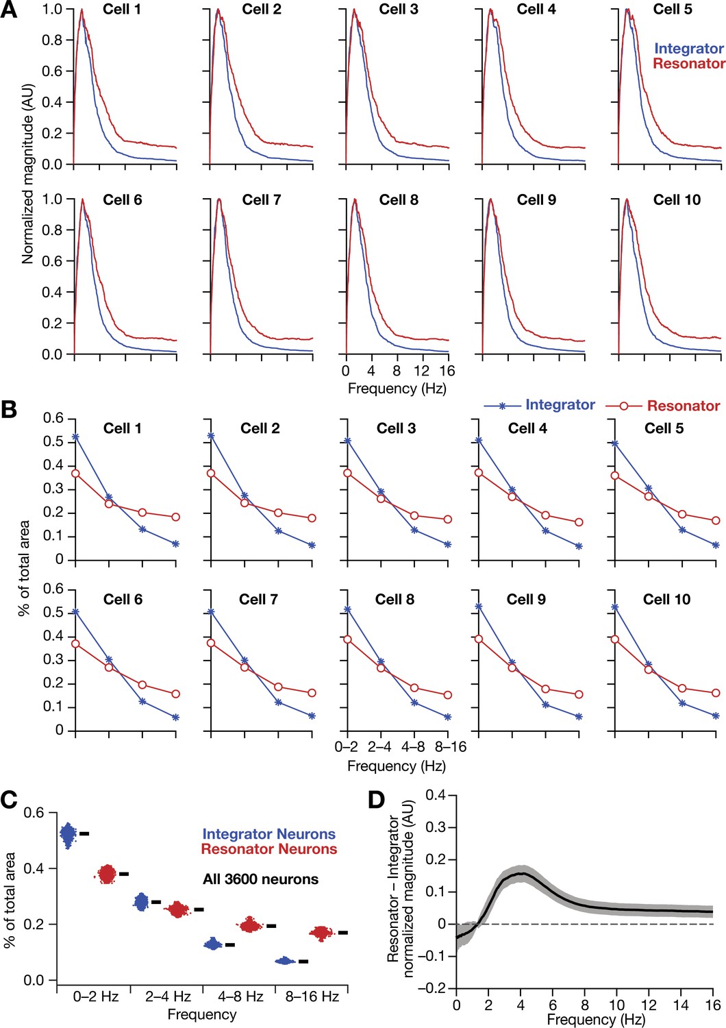
Intrinsically resonating neurons (phenomenological) suppressed low-frequency components and enhanced frequency components around resonance frequency in homogeneous CAN models.
(A–B) Ten example magnitude spectra (normalized to peak) of grid-cell activity (A) and the respective percentages of total area covered in each octave of the magnitude spectra (B) for homogeneous CAN models with integrator (blue) or resonator (red) neurons. (C) Percentage of total area covered in each octave of the magnitude spectra for homogeneous CAN models with integrator (blue) or resonator (red) neurons (n = 3600). Thick black lines represent respective median values. (D) Difference between the normalised magnitude spectra of neural temporal activity patterns for integrator and resonator neurons in a homogeneous network.
Figure 13—figure supplement 2
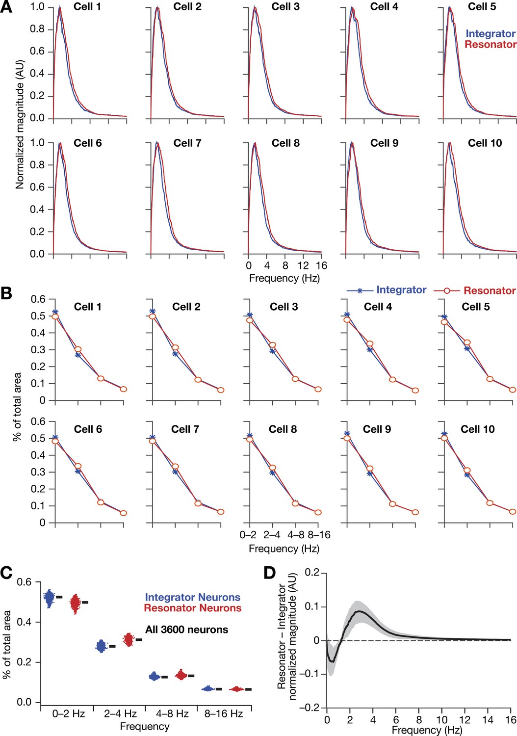
Intrinsically resonating neurons (mechanistic) suppressed low-frequency components and enhanced frequency components around resonance frequency in homogeneous CAN models.
(A, B) Ten example magnitude spectra (normalized to peak) of grid-cell activity (A) and the respective percentages of total area covered in each octave of the magnitude spectra (B) for homogeneous CAN models with integrator (blue) or resonator (red) neurons. (C) Percentage of total area covered in each octave of the magnitude spectra for homogeneous CAN models with integrator (blue) or resonator (red) neurons (n = 3600). Thick black lines represent respective median values. (D) Difference between the normalized magnitude spectra of neural temporal activity patterns for integrator and resonator neurons in a homogeneous network. Note that the mechanistic resonator does not introduce spurious high-frequency power as the phenomenological resonator (Figure 13—figure supplement 1). In terms of frequency components of neural activity, the overall impact of the mechanistic resonator on homogeneous CAN networks is minimal compared to that of the phenomenological resonator.
Figure 13—figure supplement 3
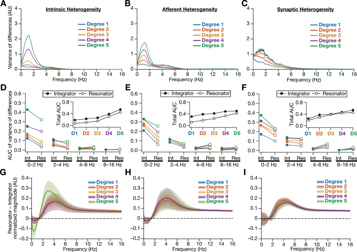
Intrinsically resonating neurons (phenomenological) suppressed heterogeneity-induced variability in low-frequency perturbations caused by different forms of biological heterogeneities.
(A–C) Normalized variance of the differences between the magnitude spectra of neurons in homogeneous vs. heterogeneous networks, across different forms and degrees of heterogeneities, plotted as a function of frequency. (D–F) Area under the curve (AUC) of the normalized variance plots shown in Figure 4 (for integrators) and (A–B) (for resonators) showing the variance to be lower in resonator networks compared to integrator networks. Panels depict outcomes for networks with different degrees of intrinsic (D), afferent (E), and synaptic (F) heterogeneities. The respective insets show the total AUC across all frequencies for the integrator vs. the resonator networks. (G–I) Difference between the normalized magnitude spectra of neural temporal activity patterns for integrator and resonator neurons. Panels depict outcomes for networks with different degrees of intrinsic (G), afferent (H), and synaptic (I) heterogeneities. Solid lines depict the mean, and shaded area depicts the standard deviations, across all 3600 neurons.
Tables
Table 1
Forms and degrees of heterogeneities introduced in the CAN model of grid cell activity.
| Degree of heterogeneity | Intrinsic heterogeneity () | Afferent heterogeneity () | Synaptic heterogeneity () | |||
|---|---|---|---|---|---|---|
| Lower bound | Upper bound | Lower bound | Upper bound | Lower bound | Upper bound | |
| 1 | 8 | 12 | 35 | 55 | 0 | 300 |
| 2 | 6 | 14 | 25 | 65 | 0 | 600 |
| 3 | 4 | 16 | 15 | 75 | 0 | 900 |
| 4 | 2 | 18 | 5 | 85 | 0 | 1200 |
| 5 | 1 | 20 | 0 | 100 | 0 | 1500 |
Additional files
-
Source code 1
Source code for simulations reported in eLife.66804.
- https://cdn.elifesciences.org/articles/66804/elife-66804-code1-v2.zip
-
Transparent reporting form
- https://cdn.elifesciences.org/articles/66804/elife-66804-transrepform-v2.pdf
Download links
A two-part list of links to download the article, or parts of the article, in various formats.
Downloads (link to download the article as PDF)
Open citations (links to open the citations from this article in various online reference manager services)
Cite this article (links to download the citations from this article in formats compatible with various reference manager tools)
Resonating neurons stabilize heterogeneous grid-cell networks
eLife 10:e66804.
https://doi.org/10.7554/eLife.66804


