A general decoding strategy explains the relationship between behavior and correlated variability
- Department of Neuroscience,University of Pittsburgh, United States
- Center for the Neural Basis of Cognition, United States
- Department of Mathematics, University of Pittsburgh, United States
Figures
Figure 1

Electrophysiological data collection and decoders.
(A) Orientation change detection task with cued attention. After the monkey fixated the central spot, two Gabor stimuli synchronously flashed on (200 ms) and off (randomized 200–400 ms period) at the starting orientation until, at a random time, the orientation of one stimulus changed. To manipulate attention, the monkey was cued in blocks of 125 trials as to which of the two stimuli would change in 80% of the trials in the block, with the change occurring at the uncued location in the other 20%. (B) A cued changed orientation was randomly assigned per trial from five potential orientations. An uncued changed orientation was randomly either the median (20 trials) or largest change amount (5 trials). To compare cued to uncued changes, median orientation change trials were analyzed. (C) The activity of a neuronal population in V4 was recorded simultaneously. Plotted for Monkey 1: the location of Stimulus 2 (red circle) relative to fixation (red cross) overlapped the receptive field (RF) centers of the recorded units (black circles). A representative RF size is illustrated (dashed circle). Only orientation changes at the RF location were analyzed. Stimulus 1 was located in the opposite hemifield (gray circle). (D) Schematic of the specific decoder, a linear classifier with leave-one-out cross-validation, which was trained to best differentiate the V4 neuronal population responses to the median changed orientation from the V4 responses to the starting orientation presented immediately before it (first and second principal components [PC] shown for illustrative purposes). (E) Schematic of the monkey’s decoder, which was based on the same neuronal population responses as in (D) but was trained to best differentiate the V4 responses when the monkey made a saccade (indicating it detected an orientation change) from the V4 responses when the monkey did not choose to make a saccade.
Figure 2 with 1 supplement
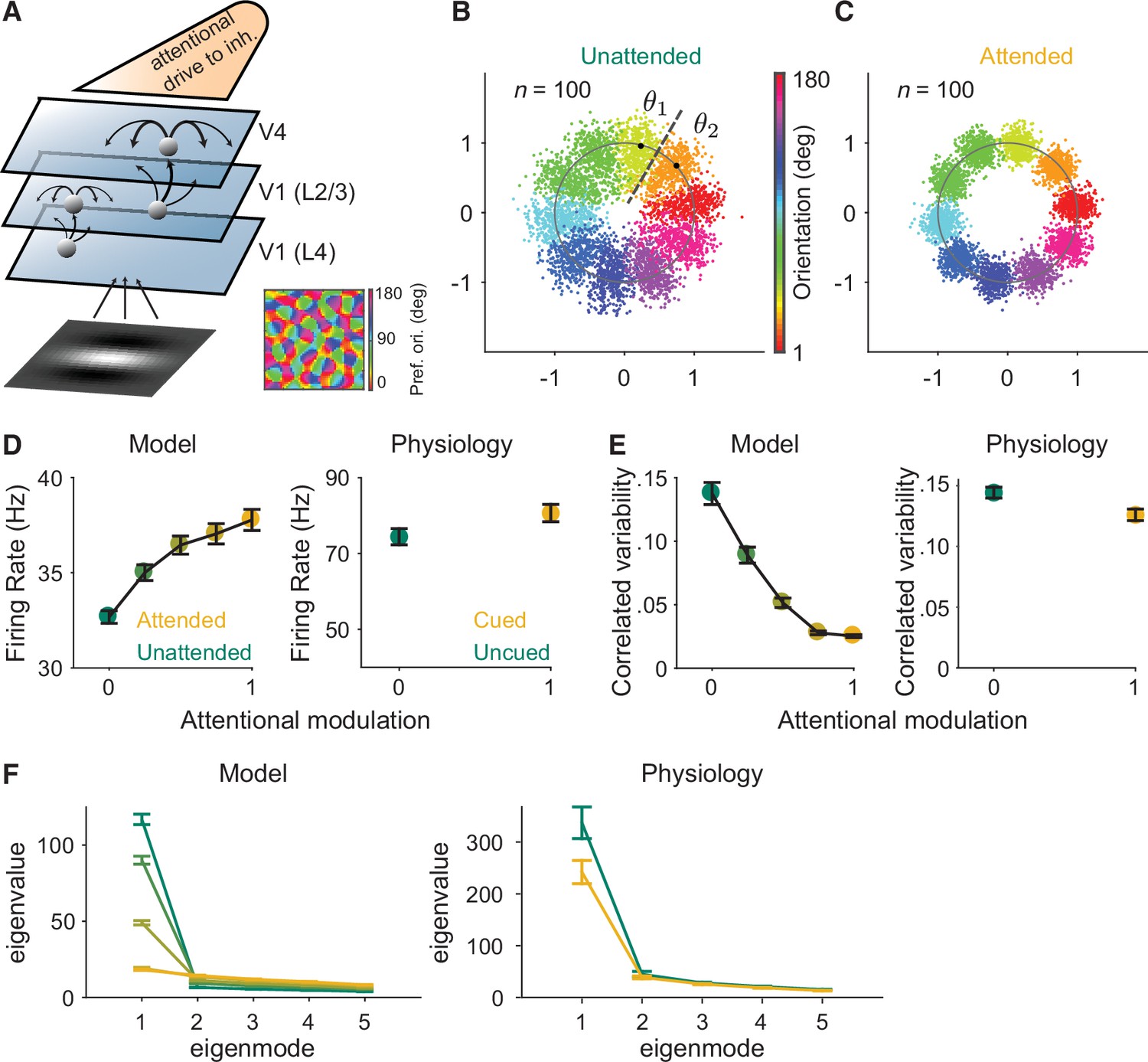
Mechanistic circuit model of attention effects.
(A) Schematic of an excitatory and inhibitory neuronal network model of attention (Huang et al., 2019) that extends the three-layer, spatially ordered network to include the orientation tuning and organization of V1. The network models the hierarchical connectivity between layer 4 of V1, layers 2 and 3 of V1, and V4. In this model, attention depolarizes the inhibitory neurons in V4 and increases the feedforward projection strength from layers 2 and 3 of V1 to V4. (B, C) We mapped the n-dimensional neuronal activity of our model to a two-dimensional space (a ring). Each dot represents the neuronal activity of the simulated population on a single trial and each color represents the trials for a given orientation. These fluctuations are more elongated in the (B) unattended state than in the (C) attended state. We then calculated the effects of these attentional changes on the performance of specific and general decoders (see Materials and methods). The axes are arbitrary units. (D–F) Comparisons of the modeled versus electrophysiologically recorded effects of attention on V4 population activity. (D) Firing rates of excitatory neurons increased, (E) mean correlated variability decreased, and (F) as illustrated with the first five largest eigenvalues of the shared component of the spike count covariance matrix from the V4 neurons, attention largely reduced the eigenvalue of the first mode. Attentional state denoted by marker color for the model (yellow: most attended; green: least attended) and electrophysiological data (yellow: cued; green: uncued). For the model: 30 samplings of n=50 neurons. Monkey 1 data illustrated for the electrophysiological data: n=46 days of recorded data. SEM error bars. Also see Figure 2—figure supplement 1.
Figure 2—figure supplement 1
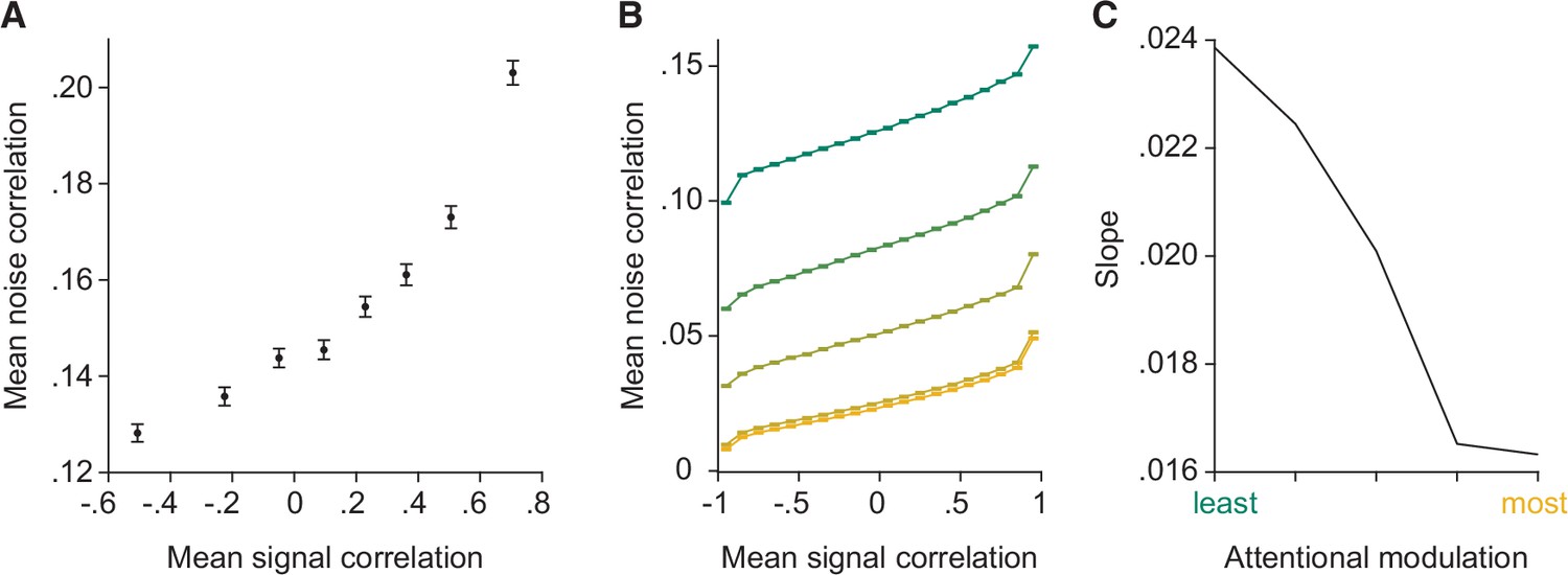
The model reproduces the relationship between noise and signal correlations that is key to the general decoder hypothesis.
(A) As previously observed in electrophysiological data (Cohen and Maunsell, 2009; Cohen and Kohn, 2011), we observe a strong relationship between noise and signal correlations. During additional recordings collected during most recording sessions (for Monkey 1 illustrated here, n=37 days with additional recordings), the monkey was rewarded for passively fixating the center of the monitor while Gabors with randomly interleaved orientations were flashed at the receptive field location (‘Stim 2’ location in Figure 1C). The presented orientations spanned the full range of stimulus orientations (12 equally spaced orientations from 0° to 330°). We calculated the signal correlation for each pair of units based on their mean responses to each of the 12 orientations. We define the noise correlation for each pair of units as the average noise correlation for each orientation. The plot depicts signal correlation as a function of noise correlation across all recording sessions, binned into eight equally sized sets of unit pairs. Error bars represent SEM. (B) The model reproduces the relationship between noise and signal correlations. Signal correlation is plotted as a function of noise correlation, binned into 20 equally sized sets of unit pairs (n=2000 neurons), for each attentional modulation strength (green: least attended; yellow: most attended). The results were averaged over 50 tested orientations. (C) The slope of the relationship between noise and signal correlations (y-axis) decreases with increasing attentional modulation (x-axis). This suggests that noise is less aligned with signal correlation with increasing attentional modulation.
Figure 3 with 2 supplements
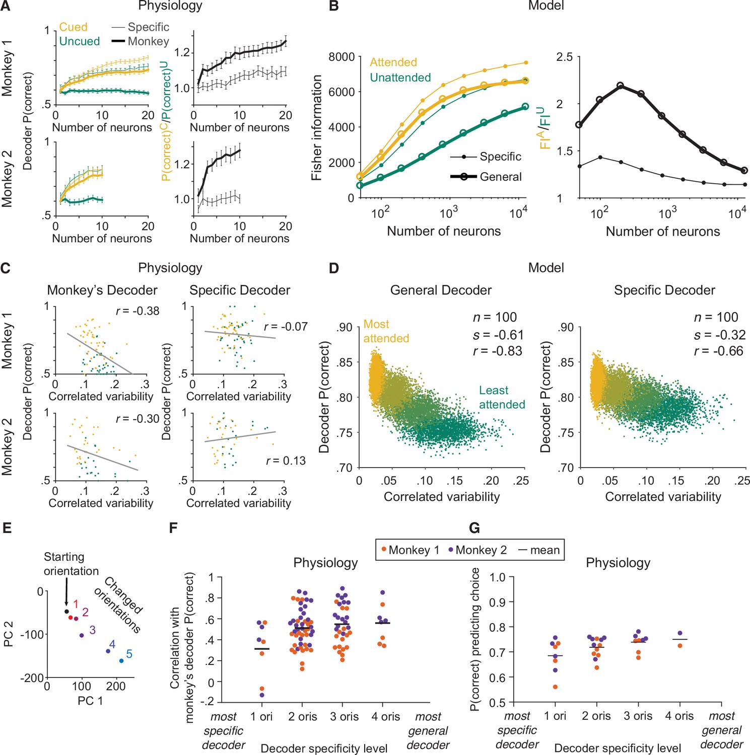
The monkey’s decoding strategy was most closely matched by a general decoding strategy.
(A) Physiological data for Monkey 1 and Monkey 2: the effect of attention on decoder performance was larger for the monkey’s decoder than for the specific decoder. Left plots: decoder performance (y-axis; leave-one-out cross-validated proportion of trials in which the orientation was correctly identified: starting versus median changed orientation) for each neuronal population size (x-axis) is plotted for the specific (thin lines) and monkey’s (thick lines) decoders in the cued (yellow) and uncued (green) attention conditions. Right plots: the ratio of the decoder performance in the cued versus uncued conditions is plotted for each neuronal population size. SEM error bars (Monkey 1: n=46 days; Monkey 2: n=28 days). (B) Modeled data: the effect of attention on decoder performance was larger for the general decoder than for the specific decoder. Left plot: the inverse of the variance of the estimation of theta (y-axis; equivalent to linear Fisher information for the specific decoder) for each neuronal population size (x-axis) is plotted for the specific decoder (small markers; Equation 1, see Materials and methods) and for the general decoder (large markers; Equation 3, see Materials and methods) in the attended (yellow) and unattended (green) conditions. Right plot: the ratio of Fisher information in the attended versus unattended conditions is plotted for each neuronal population size. (C) Physiological data for Monkey 1 and Monkey 2: the performance of the monkey’s decoder was more related to mean correlated variability (left plots, gray lines of best fit; Monkey 1 correlation coefficient: n=86, or 44 days with two attention conditions plotted per day and two data points excluded – see Materials and methods, r=–0.38, p=5.9 × 10⁻⁴; Monkey 2: n=54, or 27 days with two attention conditions plotted per day, r=–0.30, p=0.03) than the performance of the specific decoder (right plots; Monkey 1 correlation coefficient: r=–0.07, p=0.53; Monkey 2: r=0.13, p=0.36). For both monkeys, the correlation coefficients associated with the two decoders were significantly different from each other (Williams’ procedure; Monkey 1: t=3.7, p=2.3 × 10⁻⁴; Monkey 2: t=3.2, p=1.4 × 10⁻³). Also see Figure 3—figure supplement 1. (D) Modeled data: the performance of the general decoder was more related to mean correlated variability (left plot) than the performance of the specific decoder (right plot; number of neurons fixed at 100 and attentional state denoted by marker color, yellow to green: most attended to least attended). (E) An example plot of the first versus second principal component (PC) of the V4 population responses to each of the six orientations presented in the session, to justify a linear decoding strategy for the more-general decoders (starting orientation illustrated in black, five changed orientations illustrated with a red-blue color gradient from smallest to largest). Though the brain may use nonlinear decoding methods, the neuronal population representations of the small range of orientations tested per day were reasonably approximated by a line; thus, linear methods were sufficient to capture decoder performance for the physiological dataset. (F) Physiological data for Monkey 1 (orange) and Monkey 2 (purple): the more general the decoder (x-axis; number of orientation changes used to determine the decoder weights, with the decoder that best differentiated the V4 responses to the starting orientation from those to one changed orientation on the far left, and the decoder that best differentiated V4 responses to the starting orientation from those to four different changed orientations on the far right), the more correlated its performance to the performance of the monkey’s decoder (y-axis; the across-days correlation between the performance of the monkey’s decoder and the performance of the decoder specified by the x-axis). Mean across all points in a column illustrated by a black horizontal line (see Materials and methods for n values). There was a significant correlation between decoder specificity level (x-axis) and the correlation with the performance of the monkey’s decoder (y-axis; correlation coefficient: r=0.25, p=0.016). (G) The more general the decoder (x-axis), the better its performance predicting the monkey’s choices on the median changed orientation trials (y-axis; the proportion of leave-one-out trials in which the decoder correctly predicted the monkey’s decision as to whether the orientation was the starting orientation or the median changed orientation). Conventions as in (F) (see Materials and methods for n values). There was a significant correlation between decoder specificity level (x-axis) and performance predicting the monkey’s choices (y-axis; correlation coefficient: r=0.44, p=0.016).
Figure 3—figure supplement 1
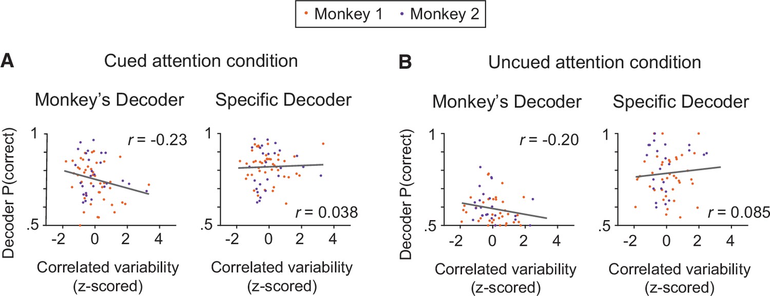
Based on the electrophysiological data, the performance of the monkey’s decoder was more related to mean correlated variability than the performance of the specific decoder within each attention condition.
(A) Within the cued attention condition, the performance of the monkey’s decoder was more related to mean correlated variability (left plot; correlation coefficient: n=71 days, r=–0.23, p=0.058) than the performance of the specific decoder (right plot; correlation coefficient: r=0.038, p=0.75). The correlation coefficients associated with the two decoders were significantly different from each other (Williams’ procedure: t=3.8, p=1.5 × 10⁻⁴). Best fit lines plotted in gray. Data from both monkeys combined (Monkey 1 data shown in orange: n=44 days; Monkey 2 data shown in purple: n=27 days) with mean correlated variability z-scored within monkey. (B) The data within the uncued attention condition showed a similar pattern, with the performance of the monkey’s decoder more related to mean correlated variability (n=69 days, r=–0.20, p=0.14) than the performance of the specific decoder (r=0.085, p=0.51; Williams’ procedure: t=2.0, p=0.049). Conventions as in (A) (Monkey 1: n=42 days – see Materials and methods for data exclusions as in Figure 3C; Monkey 2: n=27 days).
Figure 3—figure supplement 2
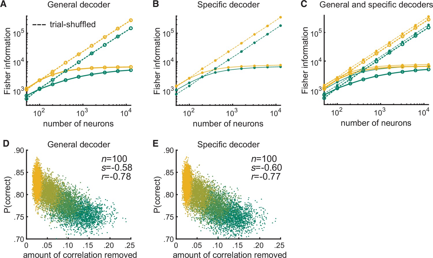
After shuffling trials, the performances of the modeled general and specific decoders and their relationships to the amount of correlated variability removed by the shuffling become indistinguishable.
(A) Randomly shuffling the trial order per neuron resulted in the Fisher information for the modeled general decoder increasing linearly with the log of the number of neurons (dashed lines) in both the attended (yellow) and unattended (green) conditions. Shuffling removes differential correlations (Moreno-Bote et al., 2014); thus, the Fisher information based on the trial-shuffled data does not saturate. (B) The trial-shuffled data resulted in the Fisher information for the modeled specific decoder increasing linearly with the log of the number of neurons (dashed lines) as well. (C) The superposition of (A) and (B) illustrates that with shuffled data, the general decoder (large markers) and the specific decoder (small markers) behave very similarly. (D) After shuffling the trials, the performances of the general decoder (E) and of the specific decoder based on the trial-shuffled data had very similar relationships to the amount of correlated variability removed by the trial shuffling (number of neurons fixed at 100 and attentional state denoted by marker color, yellow to green: most attended to least attended).
Author response image 1

Additional files
Download links
A two-part list of links to download the article, or parts of the article, in various formats.
Downloads (link to download the article as PDF)
Open citations (links to open the citations from this article in various online reference manager services)
Cite this article (links to download the citations from this article in formats compatible with various reference manager tools)
A general decoding strategy explains the relationship between behavior and correlated variability
eLife 11:e67258.
https://doi.org/10.7554/eLife.67258


