Sequence structure organizes items in varied latent states of working memory neural network
- School of Psychological and Cognitive Sciences, Peking University, China
- PKU-IDG/McGovern Institute for Brain Research, Peking University, China
- Beijing Key Laboratory of Behavior and Mental Health, Peking University, China
Figures
Figure 1

Experimental paradigm and recency effect (Experiment 1).
(A) Experiment 1 paradigm (N = 24). Subjects were first sequentially presented with two grating stimuli (1st and 2nd gratings) and needed to memorize the orientations of the two gratings as well as their temporal order (1st or 2nd orientation). During the maintaining period, a high luminance disc that does not contain any orientation information was presented as a PING stimulus to disturb the WM neural network. During the recalling period, a retro-cue first appeared to instruct subjects which item (1st or 2nd) would be tested. Next, a probe grating was presented and participants indicated whether the orientation of the probe was rotated clockwise or anticlockwise relative to that of the cued grating. (B) Grand average (mean ± SEM) behavioral accuracy for the 1st (blue) and 2nd (red) orientations. (C) Grand average (mean ± SEM) psychometric functions for the 1st (blue) and 2nd (red) items as a function of the angular difference between the probe and cued orientation. Note the steeper slope for the 2nd vs. 1st orientation, that is recency effect. (D) Scatter plot for the slope of the psychometric function for the 1st (x axis) and 2nd orientations (y axis). (*: p < 0.05).
-
Figure 1—source data 1
Source data for Figure 1.
- https://cdn.elifesciences.org/articles/67589/elife-67589-fig1-data1-v2.mat
Figure 2 with 1 supplement
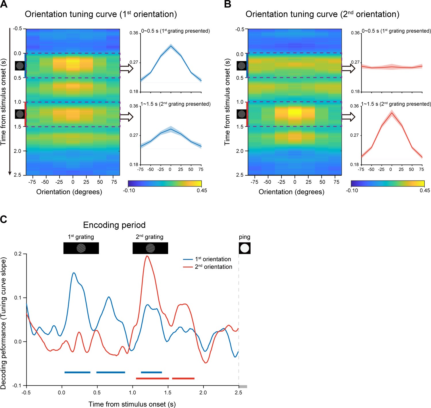
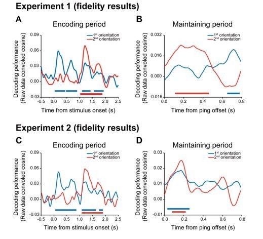
Time-resolved orientation representations during encoding period (Experiment 1).
An IEM was used to reconstruct the neural representation of orientation features, characterized as a population reconstructed channel response as a function of channel offset (x-axis) at each time bin (y-axis). Successful encoding of orientation features would show a peak at center around 0 and gradually decrease on both sides, whereas lack of orientation information would have a flat channel response. The slope of the channel response was further calculated (see Materials and methods for details) to index information representation. (A) Left: Grand average time-resolved channel response for the 1st orientation (orientation of the 1st WM grating) throughout the encoding period during which the 1st and 2nd gratings (small inset figures on the left) were presented sequentially. Right: grand average (mean ± SEM) channel response for the 1st orientation averaged over the 1st grating presentation period (0–0.5 s, upper) and the 2nd grating presentation (1–1.5 s, lower). (B) Left: Grand average time-resolved channel response for the 2nd orientation (orientation of the 2nd WM grating) during the encoding period. Right: grand average (mean ± SEM) channel response for the 2nd orientation averaged over the 1 st (0–0.5 s, upper) and 2nd (1–1.5 s, lower) grating presentation period. (C) Grand average time courses of the channel response slopes for the 1st (blue) and 2nd (red) orientations during the encoding period. Horizontal lines below indicate significant time ranges (cluster-based permutation test, cluster-defining threshold p < 0.05, corrected significance level p < 0.05) for the 1st (blue) and 2nd (red) orientations.
-
Figure 2—source data 1
Source data for Figure 2.
- https://cdn.elifesciences.org/articles/67589/elife-67589-fig2-data1-v2.mat
Figure 2—figure supplement 1
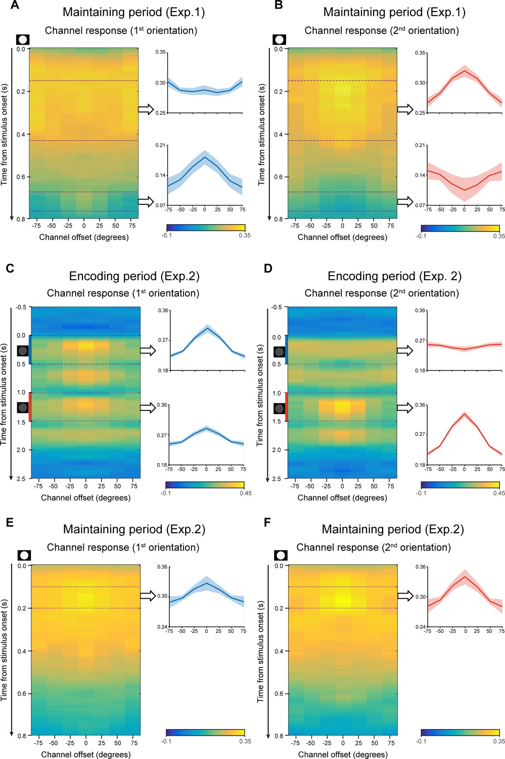
Time-resolved reconstructed channel responses.
(A–B) Maintaining period in Exp.1. (A) Grand average time-resolved channel response for the 1st orientation after the PING stimulus during the delay period (left). Grand average (mean ± SEM) channel response for the 1st orientation averaged over the 0.15–0.43 (right upper) and 0.67–0.76 s (right lower). (B) same as A, but for the 2nd item. (C–D) Encoding period in Exp.2. (C) Grand average time-resolved channel response for the 1st orientation throughout the encoding period. Grand average (mean ± SEM) channel response for the 1st orientation averaged over the 1st grating presentation period (0–0.5 s, right upper) and the 2nd grating presentation (1–1.5 s, right lower). (D) same as C, but for the 2nd item. (E–F) Maintaining period in Exp.2. (E) Grand average time-resolved channel response for the 1st orientation during the maintaining period (left). Grand average (mean ± SEM) channel response for the 1st orientation averaged over the 0.1–0.2 s (right). (F) same as E, but for the 2nd item.
Figure 3 with 3 supplements
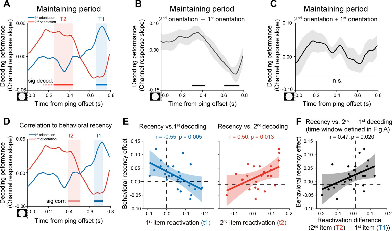
Backward reactivations during retention and behavioral relevance (Experiment 1).
(A) Grand average time courses of the channel response slope for the 1st (blue) and 2nd (red) WM orientations after PING (inset in the bottom left) during the delay period. Horizontal lines below indicate time ranges of significant decoding strengths for the 1st (blue, T1) and 2nd (red, T2) orientations, respectively. (B) Grand average (mean ± SEM) time course of the difference between the 1st and 2nd channel response slopes (2nd – 1st) and the significant time points. (C) Grand average (mean ± SEM) time course of the sum of the 1st and 2nd channel response slopes (1st + 2nd). (D) Subject-by-subject correlations between the decoding performance and the recency effect were calculated at each time point. Horizontal lines below indicate time points of significant behavioral correlations (Pearson’s correlation after multi-comparison correction) for the 1st (blue) and 2nd (red) items, respectively. (E) Left: scatterplot (N = 24) of recency effect vs. 1st decoding strength averaged over t1 (0.67–0.72 s after PING). Right: scatterplot of recency effect vs. 2nd decoding strength averaged over t2 (0.4–0.43 s after PING). (F) Scatterplot (N = 24) of recency effect vs. decoding difference (2nd at T2 – 1st at T1). Each dot represents an individual subject. (Horizontal solid line: cluster-based permutation test, cluster-defining threshold p < 0.05, corrected significance level p < 0.05; Horizontal light solid line: marginal significant, cluster-defining threshold p < 0.05, 0.05 < cluster p < 0.1); Horizontal dashed line: marginal significance, cluster-defining threshold p < 0.1, 0.05 < cluster p < 0.1. Shadow indicates 95% confidence interval.
-
Figure 3—source data 1
Source data for Figure 3.
- https://cdn.elifesciences.org/articles/67589/elife-67589-fig3-data1-v2.mat
Figure 3—figure supplement 1
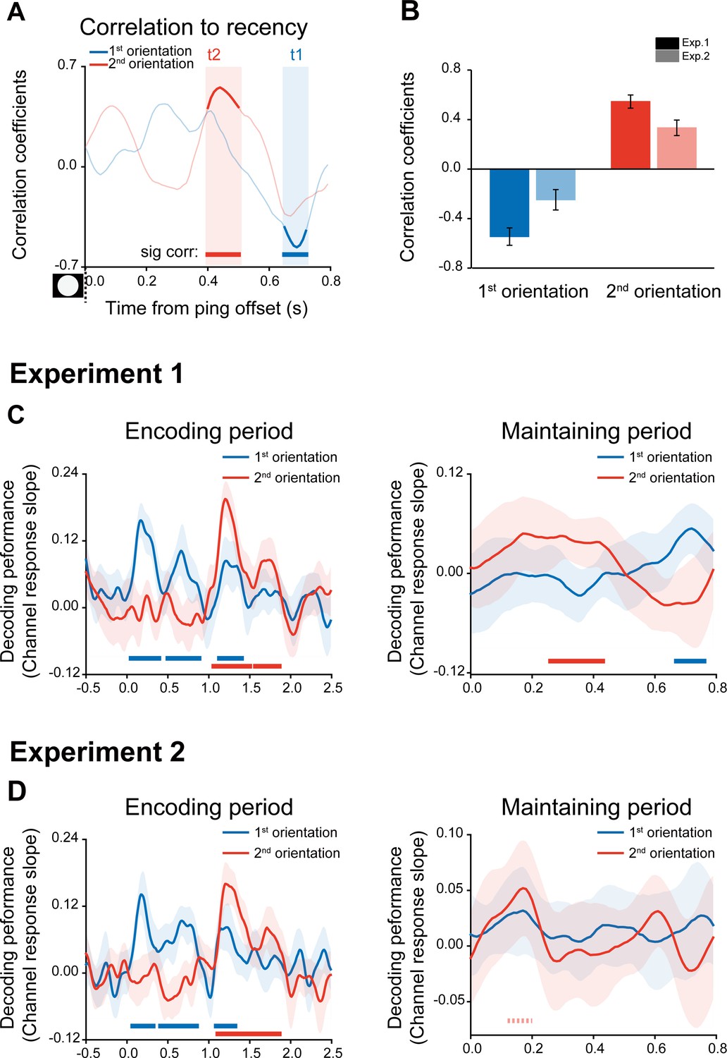
Neural-recency correlation and confidence bands for decoding time courses.
(A) Neural-recency correlation coefficients time courses in Exp.1. Horizontal lines below indicate time points of significant behavioral correlations (Pearson’s correlation after multi-comparison correction) for the 1st (blue) and 2nd (red) items, respectively. (B) Correlation coefficients between recency and reactivation strength (Mean ± 95% confidence interval) for 1st (t1, dark blue for Exp.1, light blue for Exp.2) and 2nd items (t2, dark red for Exp.1, light red for Exp.2). The confidence intervals were calculated using a jackknife procedure. (C) Grand average (Mean ± 95% confidence interval) time courses of channel response slope for the 1st (blue line) and 2nd (red line) orientations during encoding (left) and maintaining period (right) in Exp.1. (D) The same as C, but for Exp.2. (Horizontal solid line: cluster-based permutation test, cluster-defining threshold p < 0.05, corrected significance level p < 0.05; Horizontal dashed line: marginal significance, cluster-defining threshold p < 0.1, 0.05 < cluster p < 0.1).
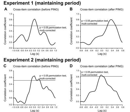
Figure 3—figure supplement 2
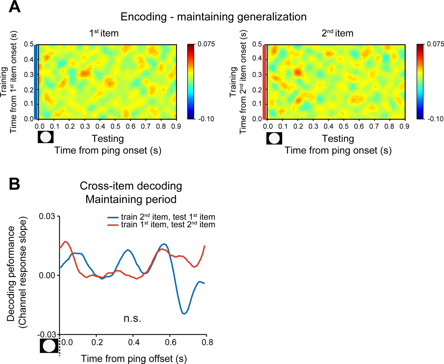
Cross-generalization results (Exp.1).
(A) Encoding-to-maintaining generalization matrices for the 1st (left) and 2nd (right) orientations by training decoders on each time point of the encoding period (y-axis) and testing all time points of the maintaining period (x-axis). (B) Cross-item generalization during the maintaining period. Blue line indicates training decoder based on the 2nd item and testing on the 1st item. Red line indicates training decoder based on the 1st item and testing on the 2nd item.
Figure 3—figure supplement 3
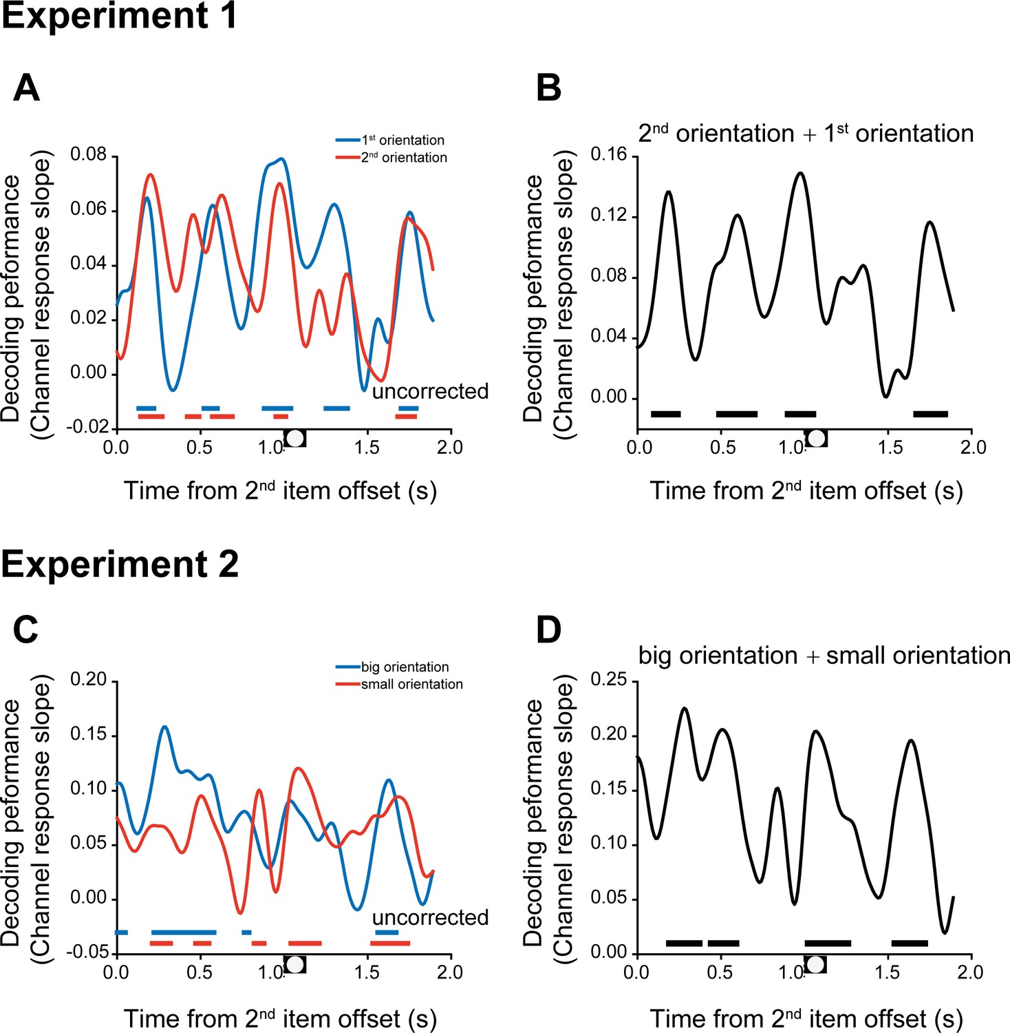
Decoding performance based on alpha-band power.
(A) Grand average decoding performance for the 1st (blue line) and 2nd (red line) orientations after the disappearance of 2nd grating. Horizontal solid line: p < 0.05, uncorrected. (B) Grand average time course of the sum of 1st and 2nd decoding performance. Horizontal solid line: cluster-based permutation test, cluster-defining threshold p < 0.05, corrected significance level p < 0.05. (C) Same as A, but for Experiment 2 in terms of big (blue line) and small (red line) orientations. (D) Same as B, but for Experiment 2 in terms of sum of big and small orientations. Note that the alpha-band decoding analysis was based on the same posterior channels used in previous analysis.
Figure 4 with 1 supplement
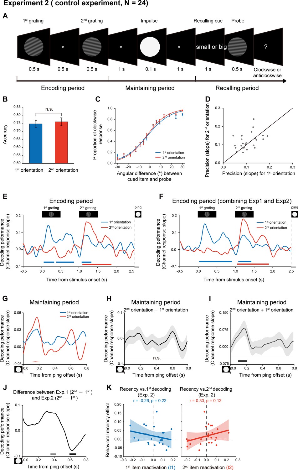
Experimental paradigm and results (Experiment 2).
(A) Experiment 2 (N = 24) had the same stimuli and paradigm as Experiment 1, except that subjects did not need to retain the temporal order of the two orientation features. Subjects were first sequentially presented with two grating stimuli (1st and 2nd gratings) and needed to memorize the two orientations. During the recalling period, a retro-cue (small or big in character) appeared to instruct subjects which item that has either smaller or larger angular values relative to the vertical axis in a clockwise direction would be tested later. Next, a probe grating was presented and participants indicated whether the orientation of the probe was rotated clockwise or anticlockwise relative to that of the cued grating. (B) Grand average (mean ± SEM) behavioral accuracy for the 1st (blue) and 2nd (red) orientations. (C) Grand average (mean ± SEM) psychometric functions for the 1st (blue) and 2nd (red) orientations as a function of the angular difference between the probe and cued orientation. (D) Scatter plot for the slope of the psychometric function for the 1st (x axis) and 2nd (y axis) orientations. (E) Grand average time courses of the channel response slopes for the 1st (blue) and 2nnd(red) orientations during the encoding period. Horizontal lines below indicate significant time points for the 1st (blue) and 2nd (red) orientations. (F) The same as E, but pooling Experiment 1 and Experiment 2 together during the encoding period (N = 48). (G) Grand average time courses of the channel response slope for the 1st (blue) and 2nd (red) WM orientations after PING (inset in the bottom left) during retention. (H) Grand average (mean ± SEM) time course of the difference between 1st and 2nd channel response slopes (2nd – 1st). (I) Grand average (mean ± SEM) time course of the sum of the 1st and 2nd channel response slopes (1st + 2nd) and significant time points. (J) Grand average time course of the 2nd – 1st reactivation difference between Exp 1 and Exp 2. (K) Same as Figure 3E but for Exp. 2. (Horizontal solid line: cluster-based permutation test, cluster-defining threshold p < 0.05, corrected significance level p < 0.05; Horizontal light solid line: marginal significant, cluster-defining threshold p < 0.05, 0.05 < cluster p < 0.1); Horizontal dashed line: marginal significance, cluster-defining threshold p < 0.1, 0.05 < cluster p < 0.1.
-
Figure 4—source data 1
Source data for Figure 4.
- https://cdn.elifesciences.org/articles/67589/elife-67589-fig4-data1-v2.mat
Figure 4—figure supplement 1
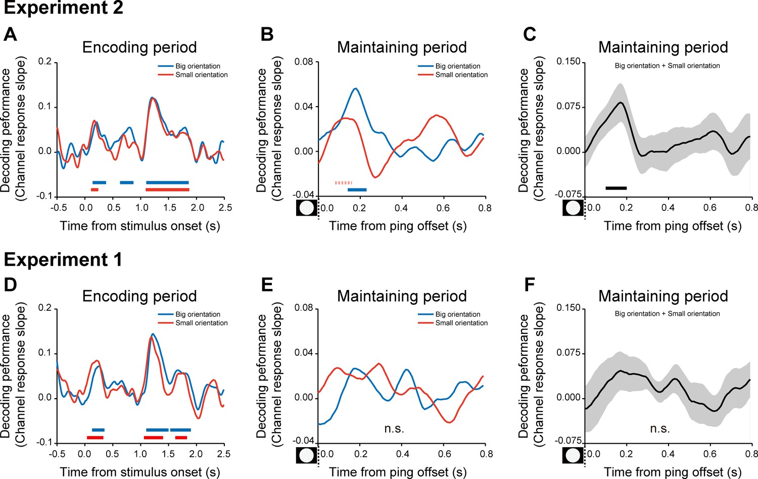
Time-resolved orientation decoding performances based on big/small label for Exp.1 and Exp.2.
(A–C) Exp.2. (A) Grand average time courses of the channel response slope for the big (blue) and small (red) orientations during the encoding period. (B) Grand average time courses of the channel response slopes for the big (blue) and small (red) orientations after the PING stimulus (inset in the bottom left) during the delay period. (C) Grand average (mean ± SEM) time course of the sum of the big and small channel response slopes (big + small) during the maintaining period. (D–F) The same as A-C, but for Exp.1. Horizontal solid line: cluster-based permutation test, cluster-defining threshold p < 0.05, corrected significance level p < 0.05; Horizontal dashed line: marginal significance, cluster-defining threshold p < 0.1, 0.05 < cluster p < 0.1. See analysis details in Materials and methods.
Figure 5
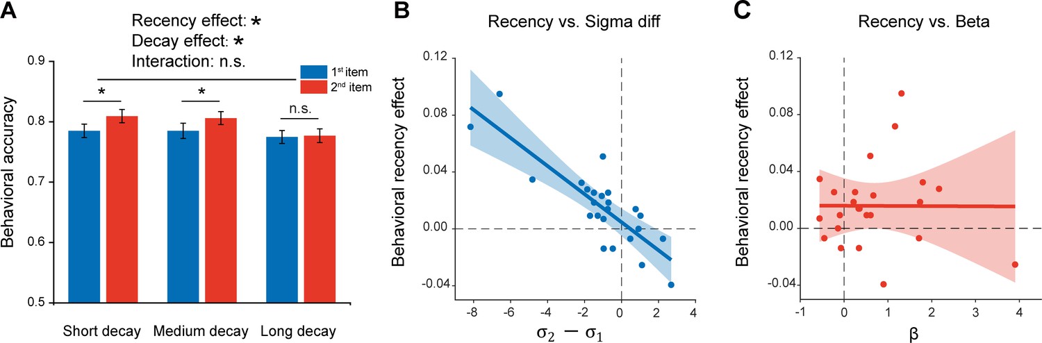
Experiment 3 and model fitting.
Experiment 3 had the same paradigm as Experiment 1, but with three levels of 2nd orientation-to-PING time intervals so that passive memory decay could be estimated. The model, endowed with sequence structure (,) and passive memory decay (β), was used to fit the behavioral data. (A) Behavioral results (N = 24). Grand averaged (mean ± SEM) behavioral accuracy for the 1st (blue) and 2nd (red) item at different 2nd orientation-to-PING time intervals. (*: Two-way repeated ANOVA (Recency × Decay), p < 0.05). (B) Sequence structure () vs. recency effect (partial correlation, r = -0.84, p < 0.001). (C) Passive memory decay (β) vs. recency effect (partial correlation, r = 0.028, p = 0.90). The results support that the recency effect mainly derives from the sequence structure rather than passive memory decay.
-
Figure 5—source data 1
Source data for Figure 5.
- https://cdn.elifesciences.org/articles/67589/elife-67589-fig5-data1-v2.mat
Author response image 1
Author response image 2
Author response image 3
Author response image 4
Author response image 5

Additional files
Download links
A two-part list of links to download the article, or parts of the article, in various formats.
Downloads (link to download the article as PDF)
Open citations (links to open the citations from this article in various online reference manager services)
Cite this article (links to download the citations from this article in formats compatible with various reference manager tools)
Sequence structure organizes items in varied latent states of working memory neural network
eLife 10:e67589.
https://doi.org/10.7554/eLife.67589


