Multiphasic value biases in fast-paced decisions
- Trinity College Institute of Neuroscience, Trinity College Dublin, Ireland
- School of Psychology, Trinity College Dublin, Ireland
- School of Electrical and Electronic Engineering and UCD Centre for Biomedical Engineering, University College Dublin, Ireland
Figures
Figure 1 with 2 supplements

Value-cued motion direction discrimination task and behavioral data.
(A) Trial structure with task conditions below. (B) Mean and standard error across participants (n = 17) for proportion correct and median response times (RTs) of correct responses. Repeated measures analyses of variance (ANOVAs) with fixed effects for task condition and value demonstrated that accuracy was higher for high-value trials than low-value trials (F(1,16) = 60.8, p < 0.001, partial η2 = 0.79), and the median RTs for correct responses were shorter (F(1,16) = 80.7, p < 0.001, partial η2 = 0.84). In addition to the large value effects, task condition affected accuracy (F(3,48) = 60.2, p < 0.001, partial η2 = 0.79) and correct RTs (F(3,48) = 38.1, p < 0.001, partial η2 = 0.61); the high-coherence conditions were more accurate (p < 0.001 for blocked and interleaved) and the blocked high-coherence condition, with the shorter deadline, was the fastest (p < 0.001 compared to other three conditions). Pairwise comparisons revealed no significant difference between the low-coherence conditions in correct RTs (p = 0.6; BF10 = 0.28). The low-coherence interleaved condition was slightly more accurate than the low-coherence blocked condition but not significantly so, and the Bayes factor indicates the data contain insufficient evidence to draw definite conclusions (p = 0.1, BF10 = 0.87). The Condition × Value interaction was significant for accuracy (F(3,48) = 6.4, p = 0.001, partial η2 = 0.29) but not correct RTs (p = 0.7).
Figure 1—figure supplement 1
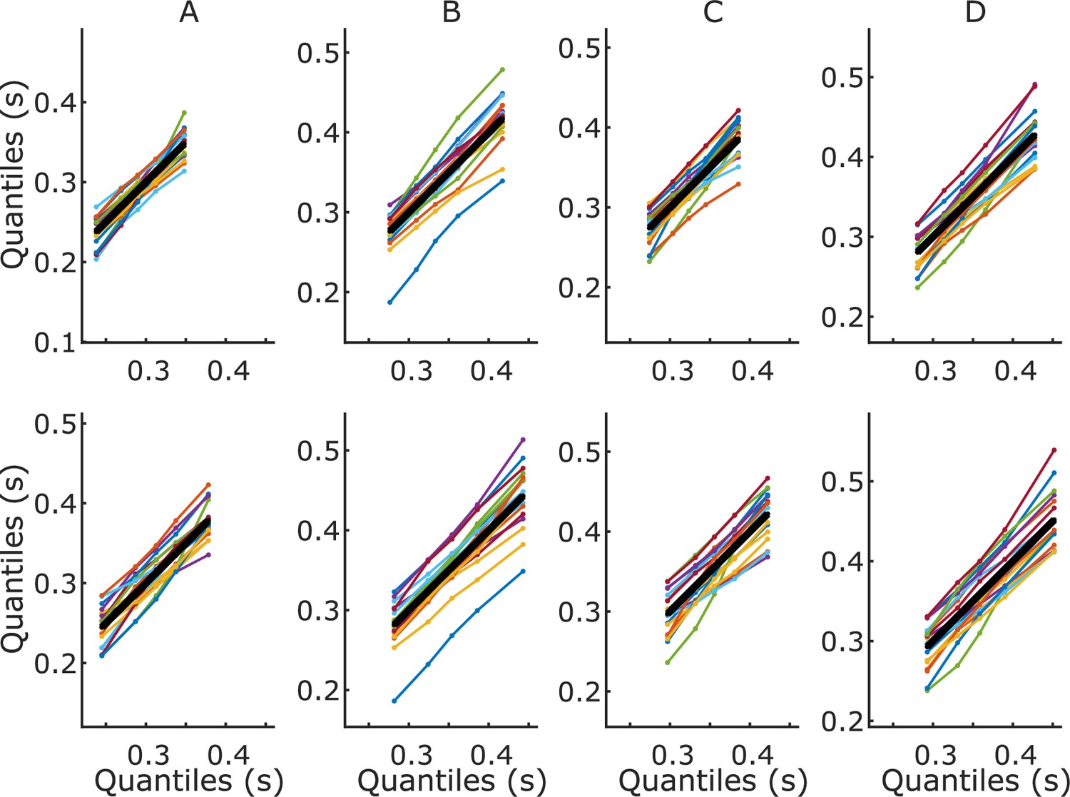
Quantile–quantile plots.
Marginal response time (RT) distribution quantiles for each participant plotted against the group-averaged quantiles, for high-value (top) and low-value (bottom) trials. The thick black line represents the group average plotted against itself. (A) High-coherence blocked; (B) low-coherence blocked; (C) high-coherence interleaved; (D) low-coherence interleaved.
Figure 1—figure supplement 2
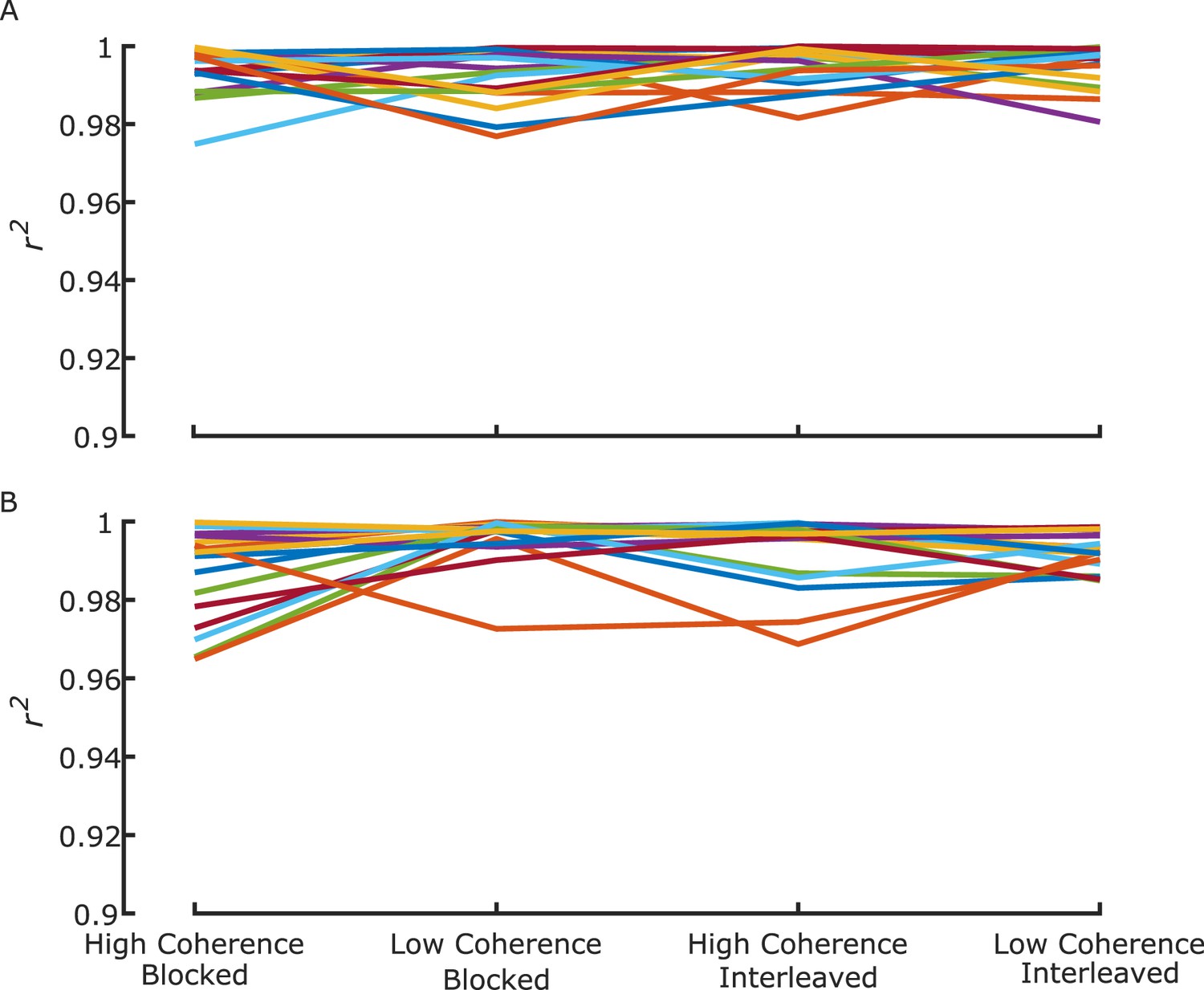
Individual-group quantile correlation (r2) statistics for (A) high-value and (B) low-value trial distributions.
Each line represents an individual participant.
Figure 2 with 2 supplements

Grand-average (n = 17) electroencephalography (EEG) signatures of motor preparation.
(A) Unilateral beta amplitude, contralateral to high- and low-value alternatives in the period after the cue and before the motion stimulus appeared at 850 or 900 ms. Note that the Y-axis is flipped such that decreasing amplitude (increasing motor preparation) is upwards. Topographies are for left-cued trials averaged with the right–left flipped topography for right-cued trials, so that the right side of the head plot represents the hemisphere contralateral to the high-value side. Amplitude topography reflects beta amplitude at 750 ms relative to amplitude at cue onset, and slope is measured from 700 to 800 ms. (B) Beta amplitude contralateral to response for correct trials only, relative to stimulus onset. Error bars are the standard errors of amplitudes 50 ms before response, with between-participant variability factored out, plotted against response time (RT). Trials were separated by session and coherence, showing high- and low-value correct trials median-split by RT and low-value error trials. (C) Relative motor preparation (the difference between the waveforms in panel A), highlighting the pre-stimulus decline due to steeper low-value urgency. (D) Lateralized readiness potential (LRP): ipsilateral–contralateral to correct response calculated at standard sites C3/C4, so that deflection upward corresponds to relative motor preparation in the correct direction. LRP waveforms were baseline corrected with respect to the interval −50 to 50 ms to focus on local stimulus-evoked dynamics. Topography shows the difference in amplitude between left- and right-cued trials at 150–180 ms relative to baseline. All waveforms derived from all trials regardless of accuracy unless otherwise stated.
Figure 2—figure supplement 1
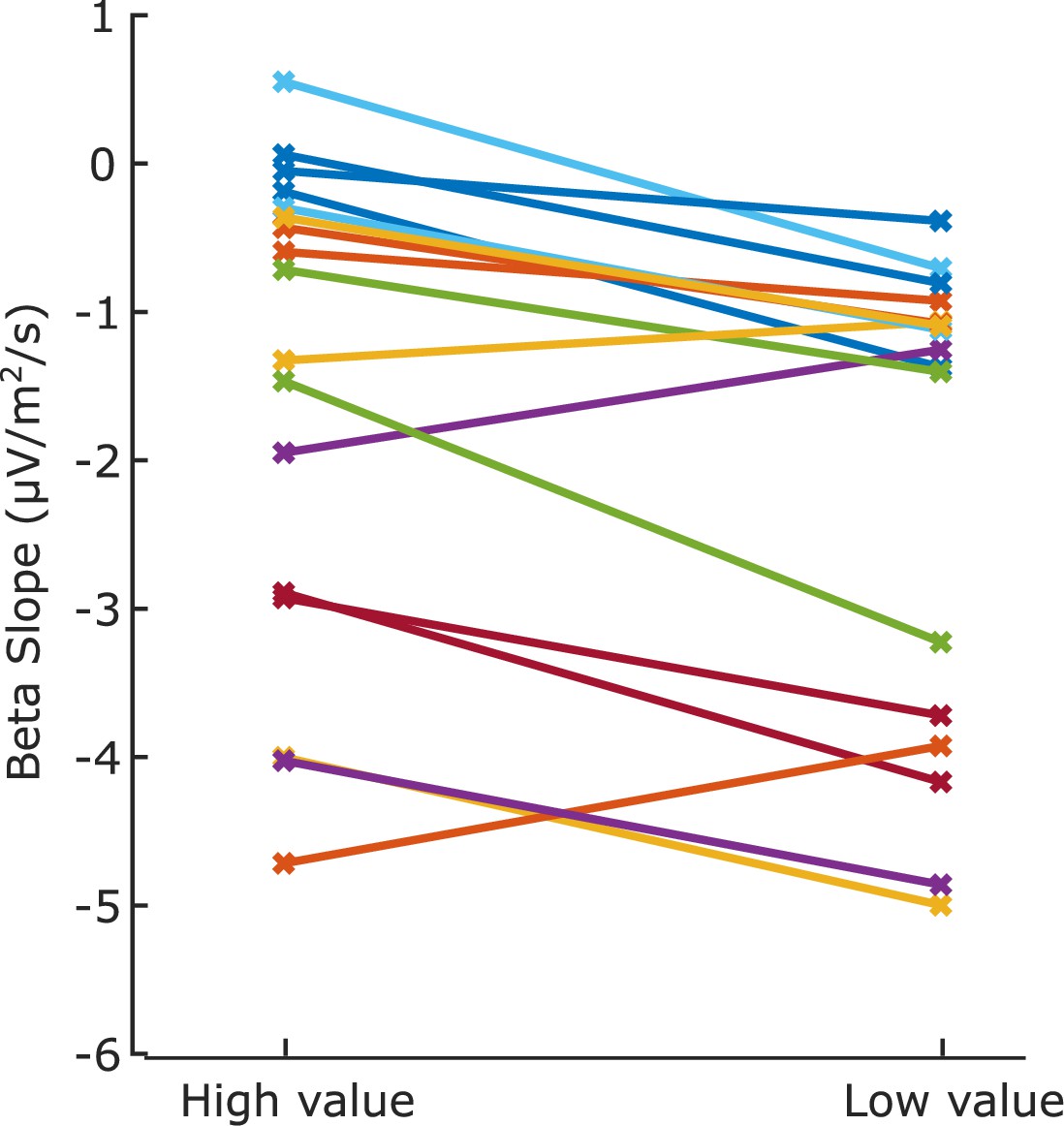
Slope of each individual’s beta decrease at 700–800 ms after the cue, for motor preparation contralateral to the high- and low-value alternatives, averaged across regimes.
Note that the slopes shown here are negative as beta is a decreasing signal. The buildup for the low-value alternative is steeper for 14 of the 17 individuals.
Figure 2—figure supplement 2
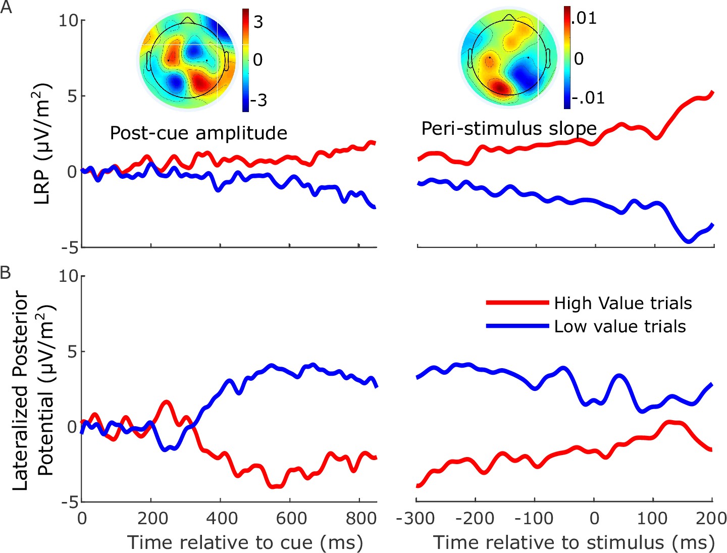
A slow-moving posterior potential interfered with measurement of the lateralized readiness potential (LRP) between cue and motion stimulus, leading us to rely solely on beta-band activity to examine anticipatory motor preparation.
Event-related potentials (ERPs) ipsilateral–contralateral to correct response, so that deflection upward corresponds to relative motor preparation in the correct direction, between cue and stimulus (left) and locked to the stimulus onset (right). (A) LRP (standard sites C3/C4—see black dots in topographies) and (B) lateralized posterior potential (calculated in the exact same way as the LRP but using parietal electrodes A5 and A18 on the left; A31 and B5 on the right, Biosemi 128-channel cap). The LRP following the onset of the cue appeared to show a slowly growing bias toward the cued direction which, contrary to our findings of a tapering relative bias in beta, persisted up to and following the stimulus onset. However, the difference topography (left inset) of left- minus right-cued trials just before stimulus onset (700 to 800 ms after the cue) relative to cue onset (−50 to 50 ms) shows that, that in addition to motor preparation, the topography was dominated by a posterior potential of the opposite polarity. This slow posterior potential begins to grow at around 300 ms after the cue and then begins to decrease after around 600 ms, calling for an accounting of potential overlap effects in interpreting the LRP dynamics between cue and stimulus. The relative beta-amplitude timecourse (Figure 2C) shows that relative preparation for the high-value alternative begins before 400 ms, at which time the LRP here appears quite stable. However, it is likely that the simultaneously increasing, opposing posterior potential may at that point be suppressing the expression of a motor preparation bias toward high value in the LRP. Then, as the relative beta preparation begins to decline at around 600 ms, the posterior potential is also beginning its decline and inducing what appears as an increasing bias to high value in the LRP. The right inset topography shows the difference in slope for left- and right-cued trials from −200 to +100 ms relative to the stimulus. It is clear that this slow drift toward high-value visible in the LRP is primarily posterior in origin. For this reason, we did not rely on the LRP to examine the anticipatory motor preparation dynamics, but rather restricted its use to the analyses of stimulus-evoked activity, and baseline corrected the signal to stimulus onset.
Figure 3
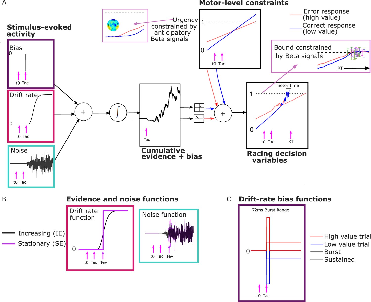
Model schematic.
(A) Components of the model with a transient burst of stimulus-evoked bias and increasing evidence (‘BurstIE’), with example traces for the cumulative sum of evidence plus bias, urgency and the resultant motor-level decision variable (DV) traces from a simulated low-value trial. A delay Tac after stimulus onset, t0, the combination of a sudden detection-triggered bias function and growing, noisy sensory evidence began to be accumulated, and with the addition of urgency drove the race between two DVs toward the threshold. The cumulative evidence plus bias was half-wave rectified such that (positive) evidence toward the correct (low-value) response was added to the low-value urgency signal, and vice versa. (B) Alternative evidence and noise functions. For stationary evidence (SE) models both stepped abruptly to their asymptotic value whereas for increasing evidence (IE) models both increased according to a gamma function. (C) Alternative drift-rate bias functions. For ‘Burst’ models the duration of bias was short, with a maximum of 72 ms, whereas sustained drift-rate bias (‘Sust’) models had a bias that continued throughout the trial. Waveforms are not drawn to scale.
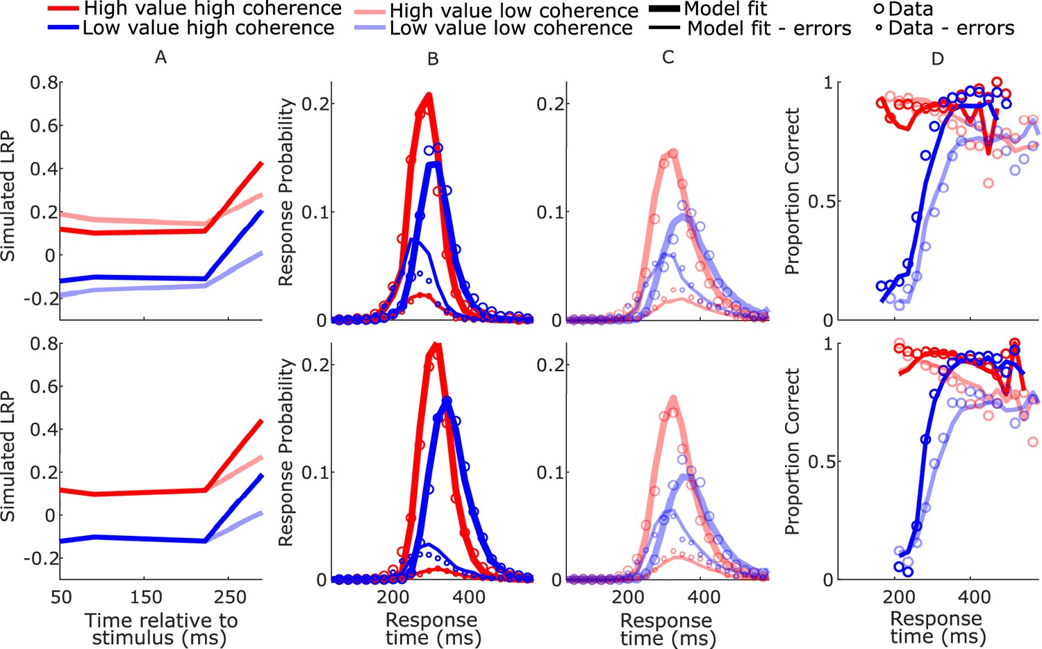
Figure 4 with 5 supplements
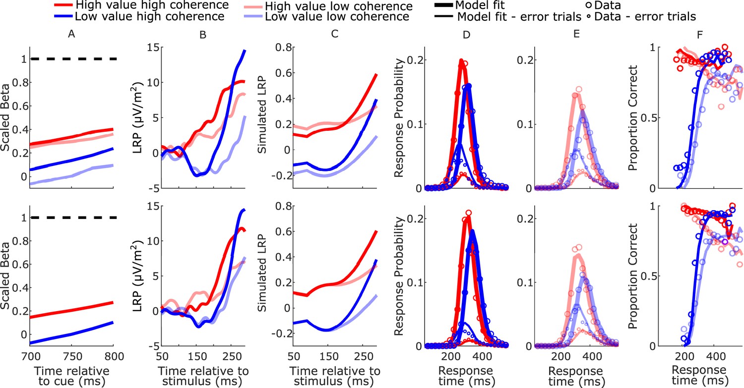
Real and model-simulated waveforms and behavior for blocked session (top row) and interleaved session (bottom row).
(A) Scaled beta signals used to constrain the models. The high- versus low-value difference in starting level varied across regime (Regime × Value interaction F(2,32) = 4.1, p = 0.03, partial η2 = 0.84; pairwise comparisons of value-difference indicated low-coherence blocked > high-coherence blocked, p = 0.01). The Regime × Value interaction for slope was not statistically significant (F(2,32) = 0.11, p = 0.89, partial η2 = 0.96); (B) real lateralized readiness potential (LRP). There was a significant interaction in bolus amplitude (mean LRP from 150 to 180 ms) between Value and Condition (F(3,48) = 2.9, p = 0.04, partial η2 = 0.16). Pairwise comparisons of the value difference provided moderate evidence that the blocked high-coherence condition had a larger difference than the interleaved high-coherence condition (p = 0.09, BF10 = 3.87); there were no significant differences between the other conditions (all p > 0.23). (C) Mean simulated trajectories of the difference between correct and incorrect decision variables (DVs) from the best-fitting model with burst drift-rate bias and increasing evidence (BurstIE); (D, E) real (circles) and model-simulated (solid lines) response time (RT) distributions. (F) Real and model-simulated conditional accuracy functions (CAFs). All waveforms derived from all trials regardless of accuracy.
Figure 4—figure supplement 1
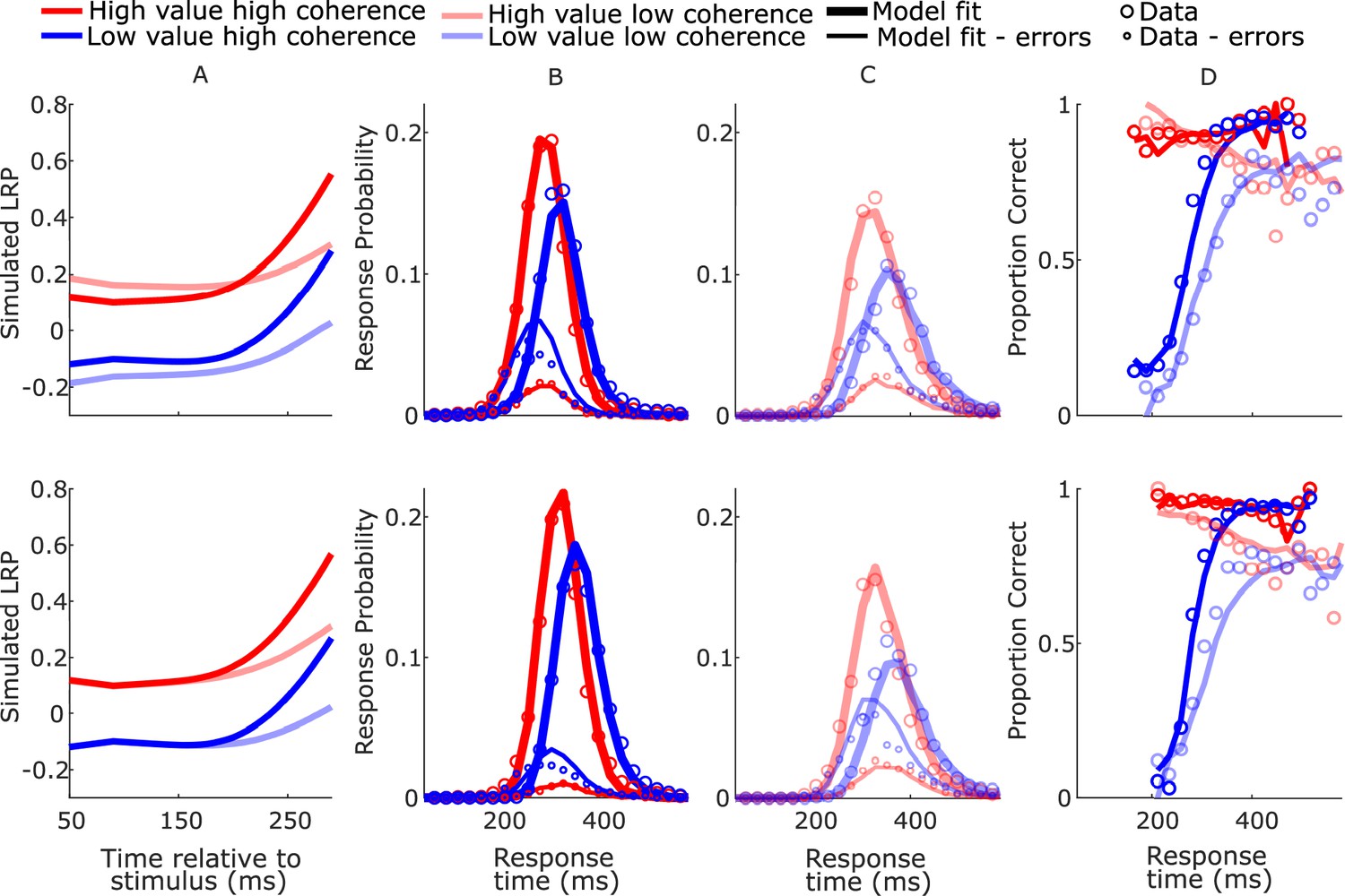
SustIE model-simulated waveforms and behavior for blocked session (top row) and interleaved session (bottom row).
(A) Mean difference between simulated decision variables (DVs); (B, C) real (circles) and model-simulated (solid lines) response time (RT) distributions. (D) Real and model-simulated conditional accuracy functions (CAFs).
Figure 4—figure supplement 2
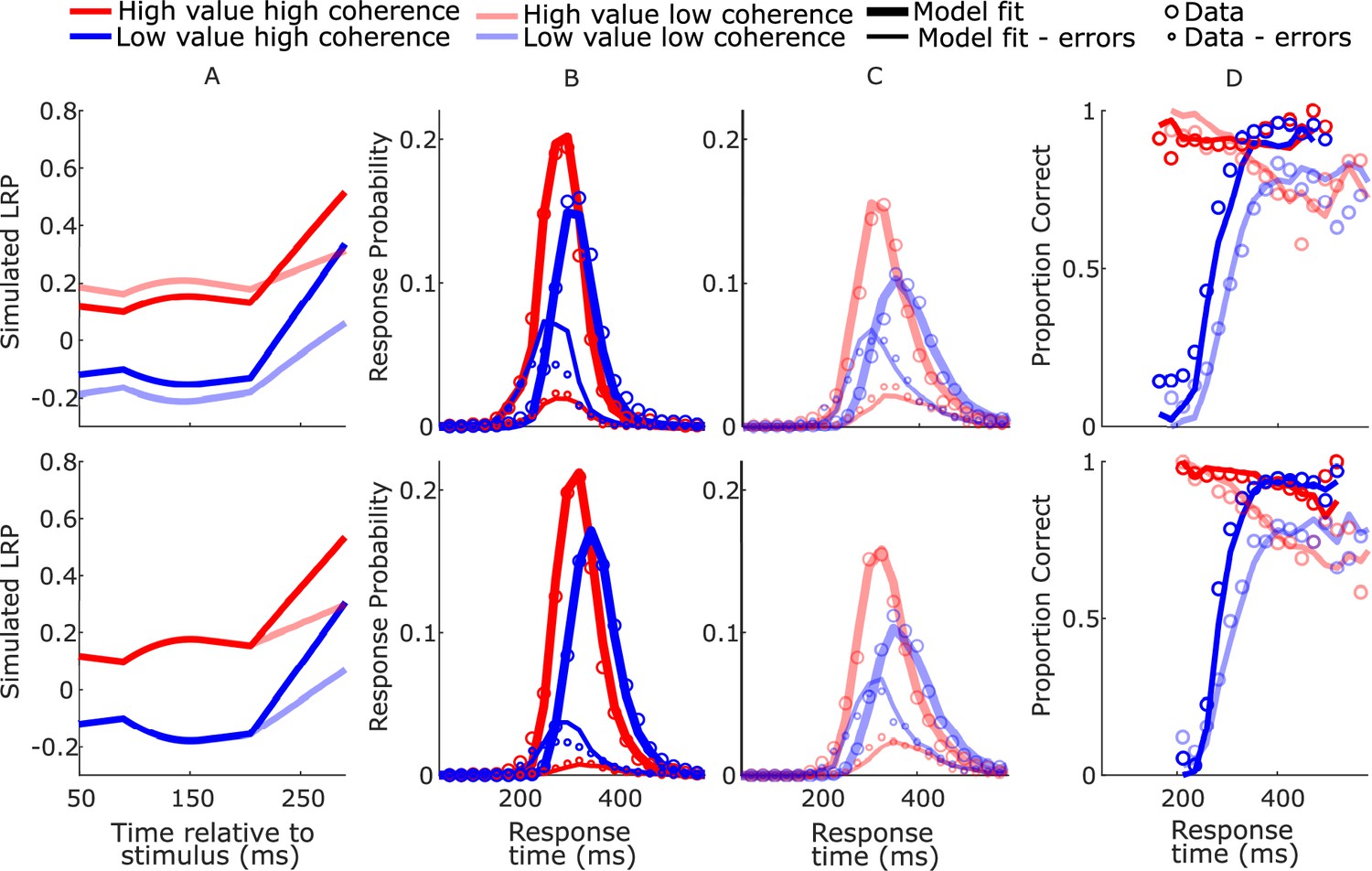
BurstSE model-simulated waveforms and behavior for blocked session (top row) and interleaved session (bottom row).
(A) Mean difference between simulated decision variables (DVs); (B, C) real (circles) and model-simulated (solid lines) response time (RT) distributions. (D) Real and model-simulated conditional accuracy functions (CAFs).
Figure 4—figure supplement 3
SustSE model-simulated waveforms and behavior for blocked session (top row) and interleaved session (bottom row).
(A) Mean difference between simulated decision variables (DVs); (B, C) real (circles) and model-simulated (solid lines) response time (RT) distributions. (D) Real and model-simulated conditional accuracy functions (CAFs).
Figure 4—figure supplement 4
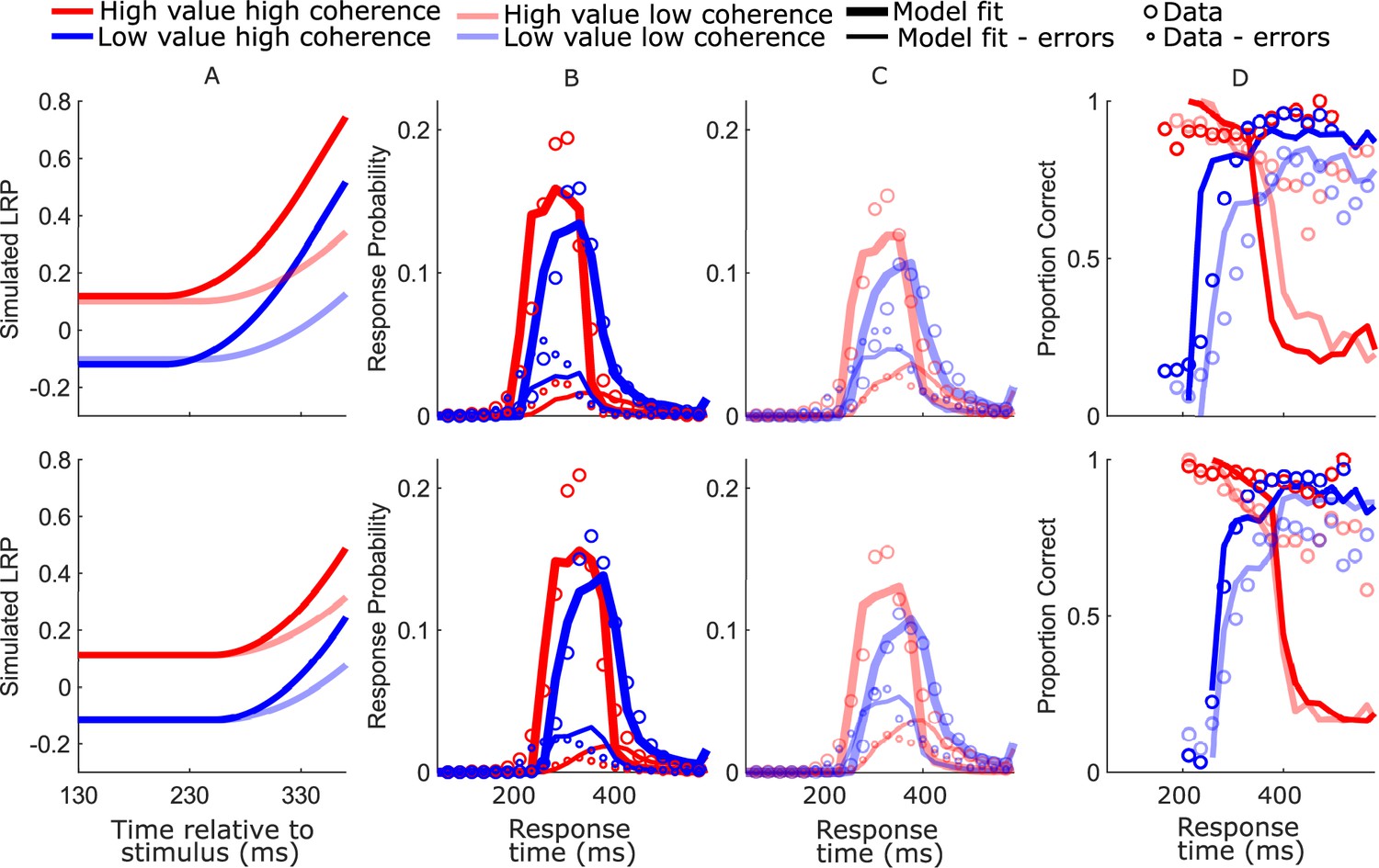
Diffusion decision model (DDM) model-simulated waveforms and behavior for blocked session (top row) and interleaved session (bottom row).
(A) Mean simulated decision variable (DV). Note the timing of the displayed DV is delayed by 80 ms relative to the neurally constrained model figures to approximately adjust for the motor component of the estimated nondecision time; (B, C) real (circles) and model-simulated (solid lines) response time (RT) distributions. (D) Real and model-simulated conditional accuracy functions (CAFs).
Figure 4—figure supplement 5
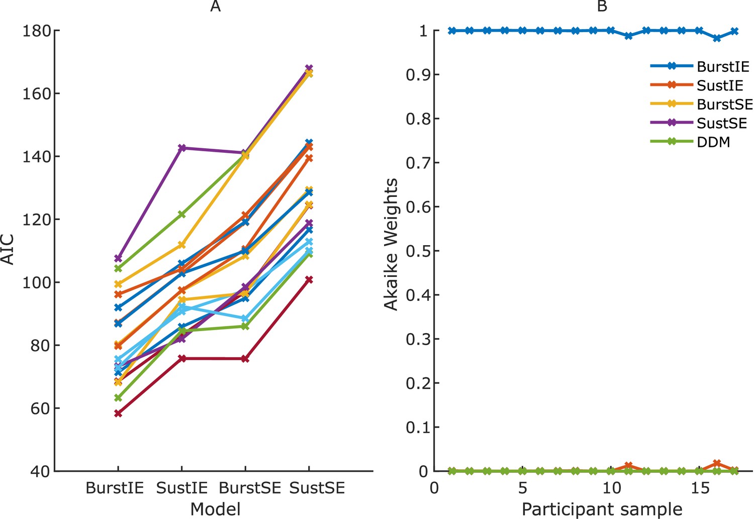
Results of Jackknifing analysis.
(A) Akaike’s information criterion (AIC) for each jackknifed sample for the four main neurally constrained models. Diffusion decision model (DDM) is excluded here to aid visibility, as its fits were markedly worse than the rest. (B) Akaike weights assigned to the five models, including DDM, for each jackknifed sample. The BurstIE model was strongly preferred for all samples.
Figure 5
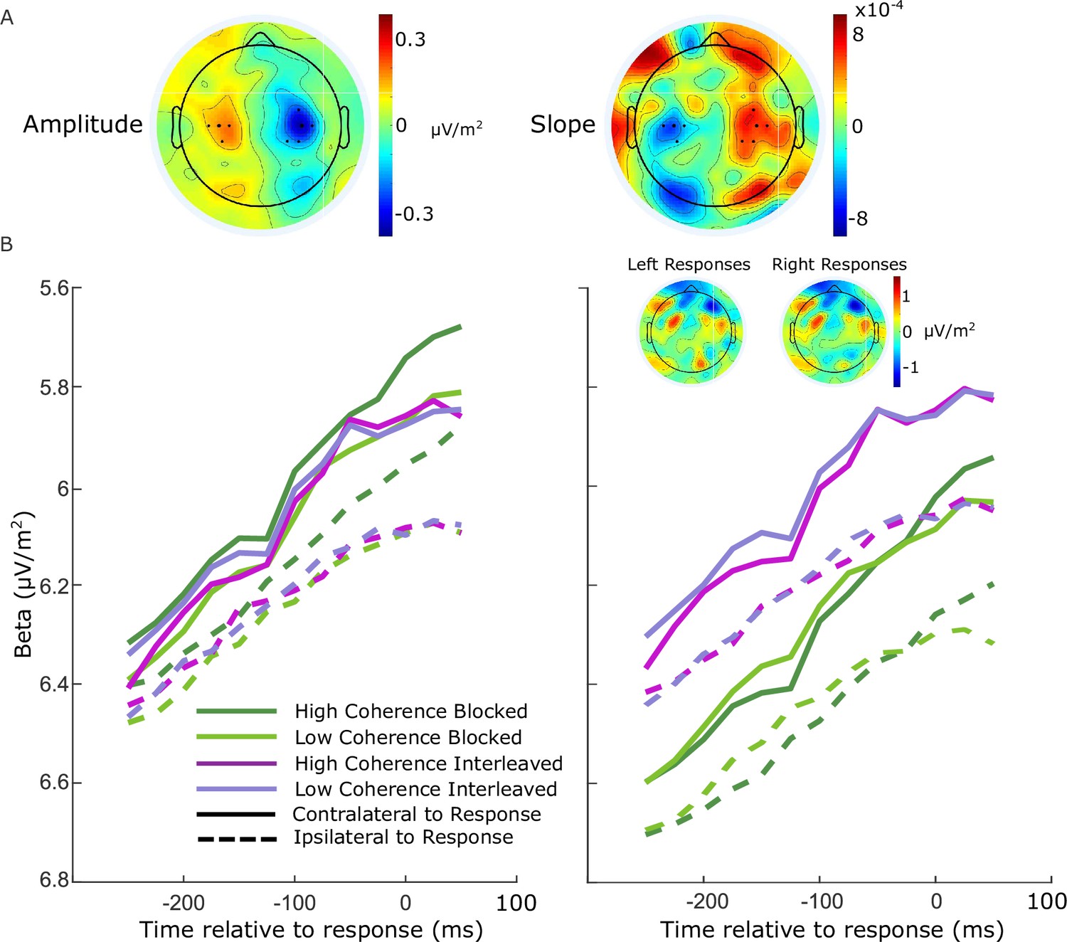
Electrode selection for beta analysis.
(A) Topographies of the difference between left- and right-cued trials for beta amplitude at 750 ms relative to amplitude at the cue, and slope from 700 to 800 ms after the cue. Standard sites C3/C4 are marked with large black dots, while other electrodes that were selected for certain individuals are marked with smaller dots. (B) Response-locked beta contralateral (solid) and ipsilateral (dashed) to response for the four conditions with individually selected electrodes. (C) Same as B, but with standard sites C3/C4 selected for all participants. Topographies show the average difference in beta amplitude between blocked and interleaved conditions at −50 ms relative to response, for right and left responses separately.
Author response image 1

Adapted from Kelly, Corbett & O’Connell 2021.
Mu/Beta motor preparation signals between a cue indicating the more probable alternative and evidence onset. The Deadline condition (red) had more speed pressure than the other two. Dynamic buildup of motor preparation began earlier in the deadline condition. The markers indicate the points at which the buildup rate of the beta signal in each regime significantly rises above zero.
Tables
Table 1
Electroencephalography (EEG)-constrained parameters.
| Parameter | Symbol | High coherence | Low coherence | Interleaved |
|---|---|---|---|---|
| Starting point contralateral to high value | Zc | 0.33 | 0.3 | 0.2 |
| Starting point ipsilateral to high value | Zi | 0.14 | 0.003 | 0 |
| Mean urgency rate contralateral to high value | Uc | 1.33 | 1.06 | 1.26 |
| Mean urgency rate ipsilateral to high value | Ui | 1.78 | 1.66 | 1.76 |
Table 2
Goodness-of-fit metrics.
| Model | Stimulus-evoked bias | Evidence | k | G2 | AIC | W |
|---|---|---|---|---|---|---|
| BurstIE | Burst | Increasing | 14 | 43 | 71 | 0.47 |
| SustIE | Sustained | Increasing | 14 | 60 | 88 | 0.0001 |
| BurstSE | Burst | Stationary | 13 | 69 | 95 | 0 |
| SustSE | Sustained | Stationary | 13 | 89 | 115 | 0 |
| Unbiased urgency slopes | Burst | Increasing | 17 | 54 | 88 | 0.0001 |
| Urgency-only bias | None | Increasing | 11 | 362 | 384 | 0 |
| DDM | None | Stationary | 14 | 606 | 634 | 0 |
| Constraints-Swap 1 | Burst | Increasing | 14 | 272 | 300 | 0 |
| Constraints-Swap 2 | Burst | Increasing | 14 | 122 | 150 | 0 |
| BurstIE + drift boost | Burst | Increasing | 15 | 42 | 72 | 0.22 |
| BurstIE + sZ | Burst | Increasing | 15 | 42 | 72 | 0.31 |
| SustIE + sZ | Sustained | Increasing | 15 | 59 | 89 | 0 |
| BurstSE + sZ | Burst | Stationary | 14 | 69 | 97 | 0 |
| SustSE + sZ | Sustained | Stationary | 14 | 92 | 120 | 0 |
| BurstSE + sTev | Burst | Stationary | 14 | 64 | 92 | 0 |
| SustSE + sTev | Sustained | Stationary | 14 | 92 | 120 | 0 |
-
Goodness-of-fit quantified by chi-squared statistic, G2. Model comparison was performed using AIC, which penalises for the number of free parameters (k). The Akaike weights (W) shown, which can be cautiously interpreted as the probability that each model is the best in the set, are calculated here based on the set of models in this table. The probability mass is shared between the different versions of the BurstIE model. In the two Constraints-Swap models, the constrained parameters for (A) high- coherence, (B) low- coherence, and (C) interleaved blocks were taken from the neural signals corresponding to [B,C,A] (Swap 1) and [C,A,B] (Swap 2), respectively.
Table 3
Estimated parameters for the four main models.
| Parameter | Symbol | BurstIE | SustIE | BurstSE | SustSE |
|---|---|---|---|---|---|
| Asymptotic drift rate (high coherence) | νh | 6.4 | 8.4 | 4.9 | 4.6 |
| Asymptotic drift rate (low coherence) | νl | 2.8 | 3.3 | 2.1 | 2.1 |
| Drift-rate bias (high-coherence blocked) | νbh | 2.4 | 0.63 | 2.3 | 0.51 |
| Drift-rate bias (low-coherence blocked) | νbl | 2.3 | 0.49 | 2.4 | 0.46 |
| Drift-rate bias (interleaved) | νbi | 3.1 | 0.74 | 3.1 | 0.63 |
| Within-trial noise asymptotic standard deviation | s | 1.13 | 1.16 | 0.93 | 0.81 |
| Accumulation onset time (ms) | Tac | 90 | 90 | 91 | 91 |
| Burst duration range (ms) | brange | 72 | — | 72 | — |
| rate | β | 54.9 | 41.4 | — | — |
| argument | n | 6.9 | 6.7 | — | — |
| Evidence onset time (ms) | Tev | — | — | 205 | 223 |
| Mean motor time (high-coherence blocked) (ms) | Trh | 86 | 72 | 73 | 57 |
| Mean motor time (low-coherence blocked) (ms) | Trl | 85 | 67 | 74 | 54 |
| Mean motor time (interleaved) (ms) | Tri | 95 | 79 | 84 | 63 |
| Urgency-rate variability | su | 0.42 | 0.46 | 0.39 | 0.4 |
| Motor time variability (ms) | st | 65 | 65 | 81 | 80 |
-
Note: Fixed parameter shown in bold typeface.
Table 4
Estimated parameters for the diffusion decision model (DDM).
| Parameter | Symbol | DDM |
|---|---|---|
| Drift rate (high coherence) | νh | 6.34 |
| Drift rate (low coherence) | νl | 3.5 |
| Bound (high-coherence blocked) | ah | 0.17 |
| Bound (low-coherence blocked) | al | 0.18 |
| Bound (interleaved) | ai | 0.16 |
| Starting point bias (high-coherence blocked) | zb_h | 0.12 |
| Starting point bias (low-coherence blocked) | zb_l | 0.1 |
| Starting point bias (interleaved) | zb_i | 0.11 |
| Nondecision time (high-coherence blocked) (ms) | Ter_h | 0.27 |
| Nondecision time (low-coherence blocked) (ms) | Ter_l | 0.3 |
| Nondecision time (interleaved) (ms) | Ter_i | 0.31 |
| Starting point variability | sz | 0.09 |
| Nondecision time variability | st | 0.13 |
| Drift-rate variability | η | 6.39 |
Table 5
Scaled beta start points and slopes for individually selected electrodes and C3/C4.
| Parameter | Individually selected | C3/C4 | ||||
|---|---|---|---|---|---|---|
| High coherence | Low coherence | Interleaved | High coherence | Low coherence | Interleaved | |
| Zc | 0.33 | 0.3 | 0.2 | 0.33 | 0.35 | 0.2 |
| Zi | 0.14 | 0.003 | 0 | 0.12 | 0.06 | 0 |
| Uc | 1.33 | 1.06 | 1.26 | 1.24 | 0.95 | 1.17 |
| Ui | 1.78 | 1.66 | 1.76 | 1.66 | 1.61 | 1.63 |
Additional files
Download links
A two-part list of links to download the article, or parts of the article, in various formats.
Downloads (link to download the article as PDF)
Open citations (links to open the citations from this article in various online reference manager services)
Cite this article (links to download the citations from this article in formats compatible with various reference manager tools)
Multiphasic value biases in fast-paced decisions
eLife 12:e67711.
https://doi.org/10.7554/eLife.67711


